1. Introduction
As the development of Location Based Services (LBSs), the GPS technique can provide reliable outdoor positioning, but it is invalid in indoor environments. Indoor positioning is required in places like hospitals, warehouses, malls and tunnels. Some commercial indoor location techniques have appeared, such as Wi-Fi fingerprint, RFID, UWB and computer vision, but indoor positioning is still not a well resolved problem so far. All these means need pre-installed infrastructures, network and remote database support. Their high cost also make it impossible to cover all the buildings. On the other hand, when a disaster strikes, the infrastructure becomes fragile. It is very difficult to track emergency first responders by traditional indoor positioning method. Fortunately, with the fast development of Micro Electro Mechanical System (MEMS), it becomes possible to realize reliable personal location for GPS-denied environments using PINS algorithm based on foot-mounted inertial measurement units (IMU). An outstanding advantage of these systems is that they are self-contained, which can compensate for the dead zones of wireless location techniques and provide seamless localization [
1,
2,
3]. This solution is very useful in many applications. For example, tracking emergency first responders [
4,
5], guiding blind people [
6] and augmenting reality. Furthermore, the IMU could be integrated into wearable sensor networks, which could provide rich context information for the future Smart World.
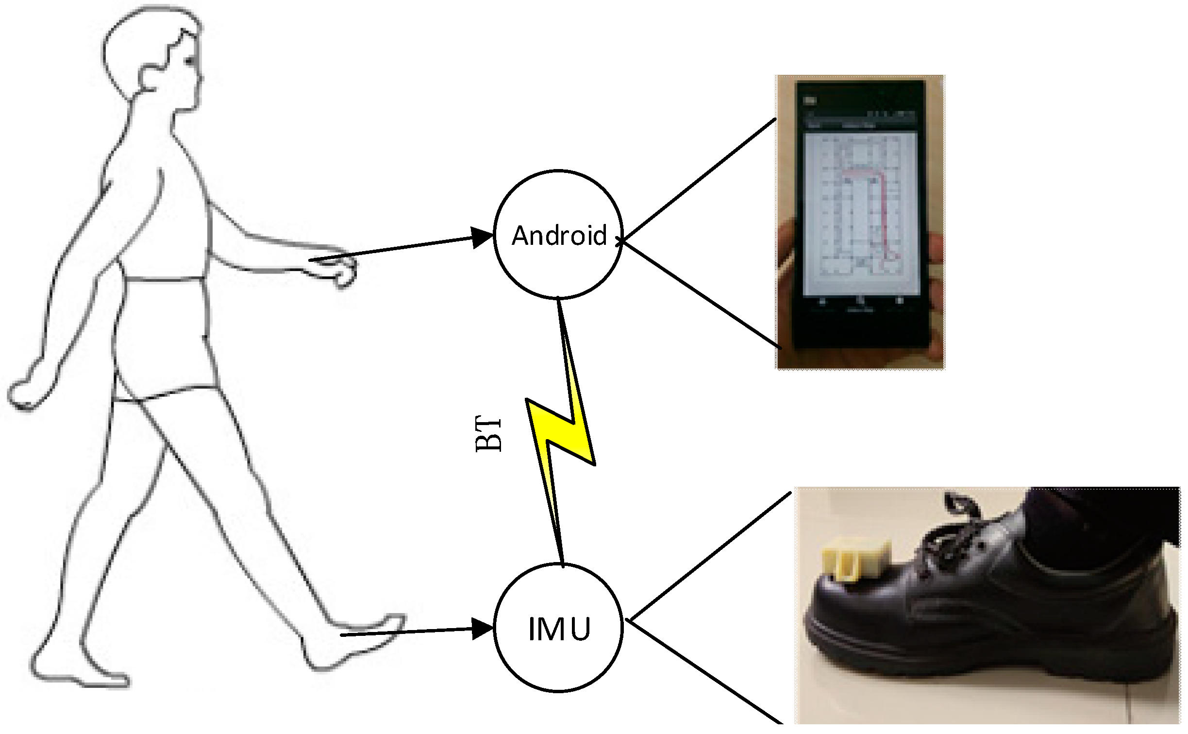
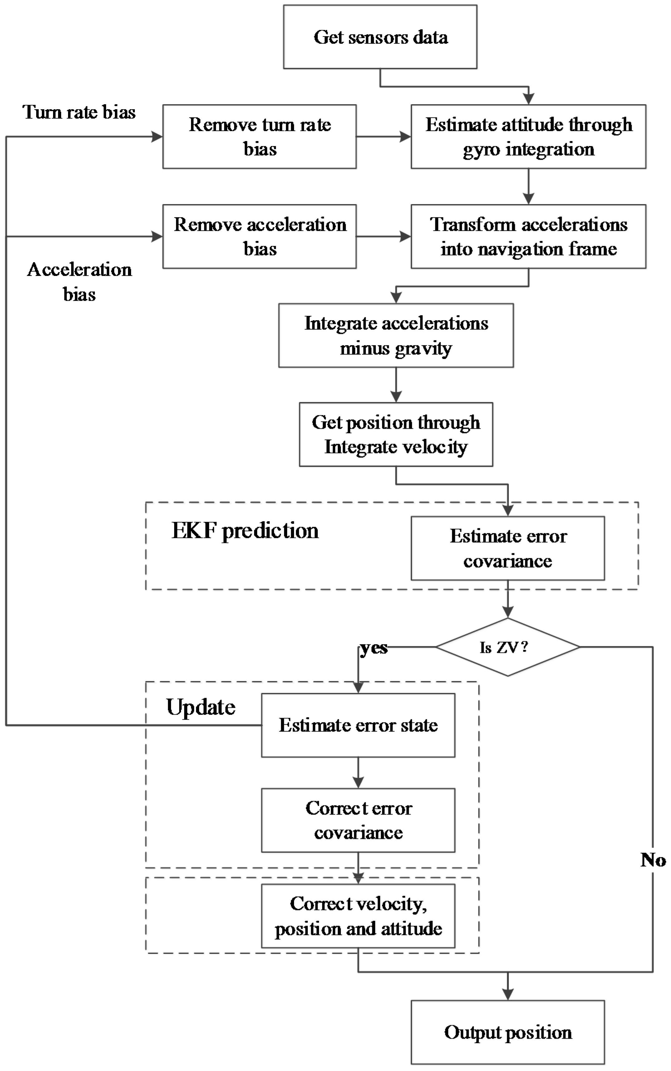
The typical PINS application framework is shown in
Figure 1. An IMU is mounted on the top of the toe and captures the movement characteristics of the foot. However the irregular movement patterns of people and lack of moving control information like unmanned vehicle systems, make it impossible to track pedestrian position using inertial sensing alone. The position error grows cubically in time brought about by double integrating acceleration errors, which will make the system collapse in the short time. However, during the detected ZV period in a gait cycle, the Zero Velocity Update (ZUPT) and Zero Angular Rate Update (ZARU) features provide pseudo measurements to error states EKF [
7,
8,
9]. This allows the EKF to correct the velocity error and attitude error after each stride, stopping the position error from grow linearly. The reason why ZUPT/ZARU could correct errors is that it tracks the growing correlations among the velocity, position and attitude errors in certain off-diagonal elements of the covariance matrix. For example, at the end of a stride, there exists a high correlation between the uncertainty in the north velocity and the newly accumulated uncertainty in the northing position. If the ZUPT suggested that the velocity error was positive in the north direction, the EKF would correct the position to the south and the velocity to zero.
Figure 1.
PINS application framework.
Figure 1.
PINS application framework.
Since the ZUPT/ZART is so important to PINS, the key problem is how to detect the ZV period accurately, which will directly affect the correction of PINS, especially to the altitude [
10]. The traditional threshold method assumes that the acceleration should be only the gravitational acceleration, and the angular rate should be zero during the ZV period, so setting a threshold on the magnitude of the rate-of-turn is applied into a ZV detector [
11]. Moreover, a combined condition method is proposed which sets threshold on the acceleration magnitude, local acceleration variance as well as gyroscope magnitude [
12], respectively:
where
,
is the measurement of an accelerometer in the three orthogonal axes at time k, and
,
is the gyroscope. Then a logical “AND” allows one to judge ZV by three conditions simultaneously. Finally, the noise in the result is filtered out using a median filter [
13]. Based on this method, a dynamic threshold is used to enhance the robustness of the system [
14,
15]. Furthermore, some probabilistic methods are introduced [
16], like the use of the HMM framework to give the probability of movement and standstill for each time instant [
17,
18]. In order to get a better detection effect, a multi-IMU platform is proposed [
19]. Some researchers adopt force sensitive resistors as external zero velocity detectors [
20]. These solutions are more reliable, but involve more complex electric designs and higher communication costs.
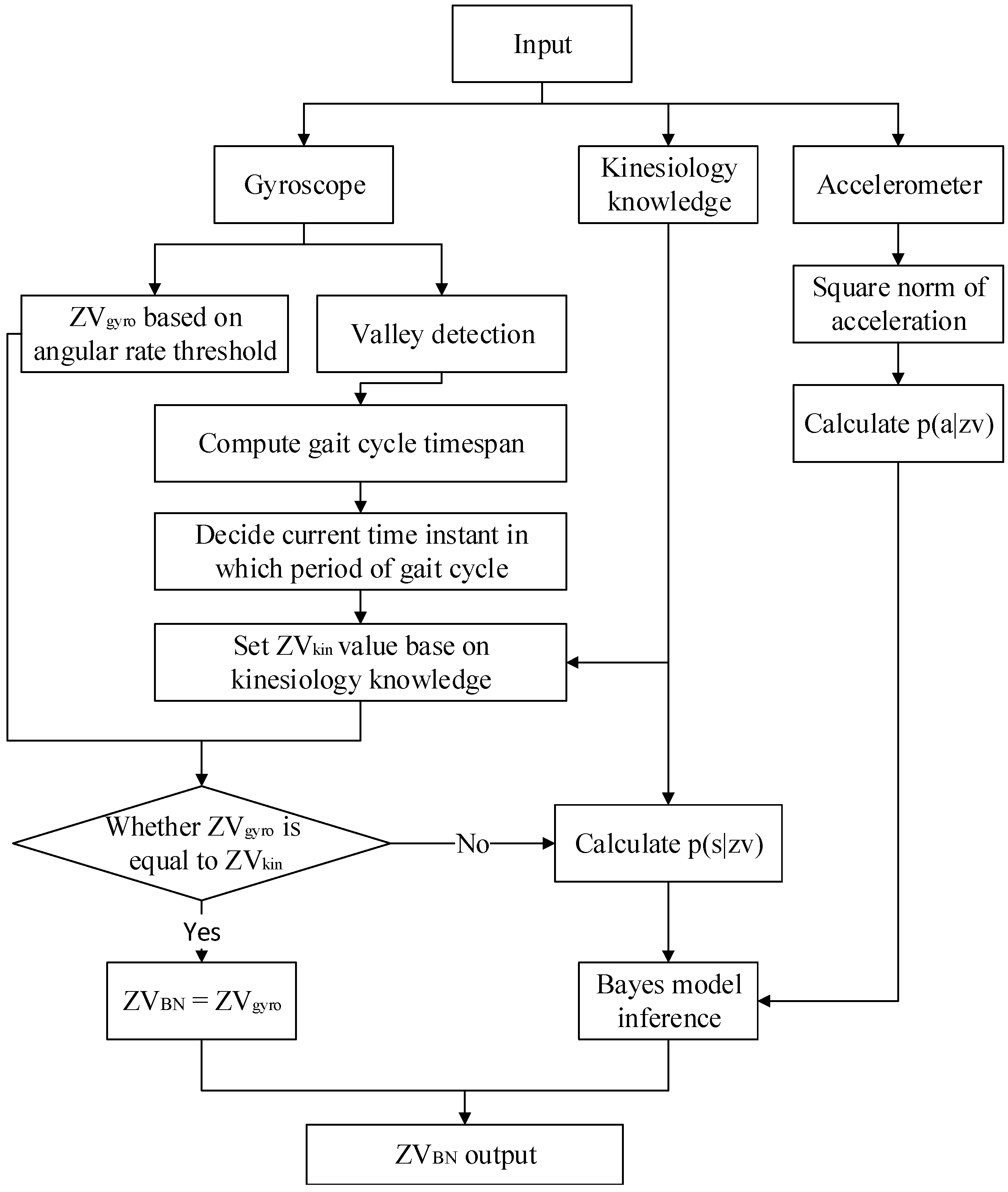
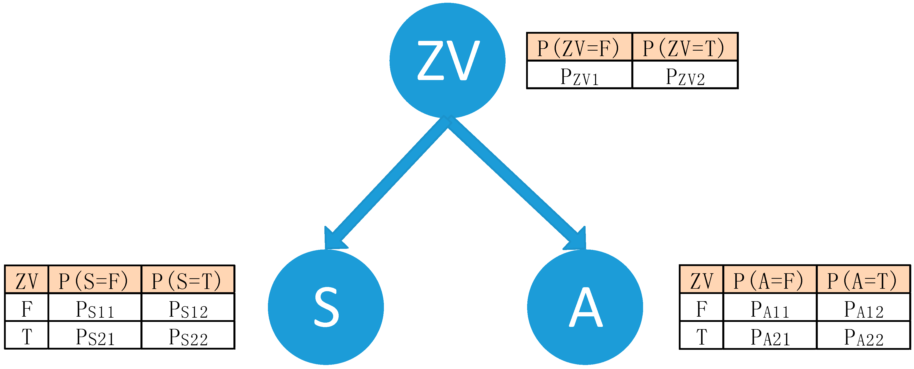
However, the ZV detectors mentioned above cannot deal with two main problems well. Firstly, the boundaries of the ZV period are fuzzy during the contact period and propulsive period in the gait cycle. Secondly, there exist ZV false detections due to the noise. The proposed solution extends the classic combined condition method, using Bayesian Network method to infer the ZV period with the measurements of low-cost IMUs and kinesiology knowledge. With a high probability of ZV, the method can remove ZV false detections effectively in the midstance period. Aided by the segmentation of the gait cycle, the method could reduce the ambiguity of ZV boundaries. The experiments reveal that the removal rate of ZV false detections increases 80% compared with the classic method at high speed. With the result of this ZV detector, a PINS/EKF aided by ZUPT/ZARU is proposed to realize 3D tracking of pedestrians. The experiments show that the method can achieve good tracking effects and decrease the altitude error by 40% compared with the PINS/EKF based on a combined condition ZV detector.
The remainder of this paper is organized as follows:
Section 2 introduces the kinesiology model and proposes a gait cycle detector algorithm.
Section 3 details the ZV detector based on Bayesian network inference.
Section 4 presents the PINS/EKF framework and
Section 5 presents experimental results. Finally,
Section 6 provides the conclusions.
2. Gait Cycle Detector
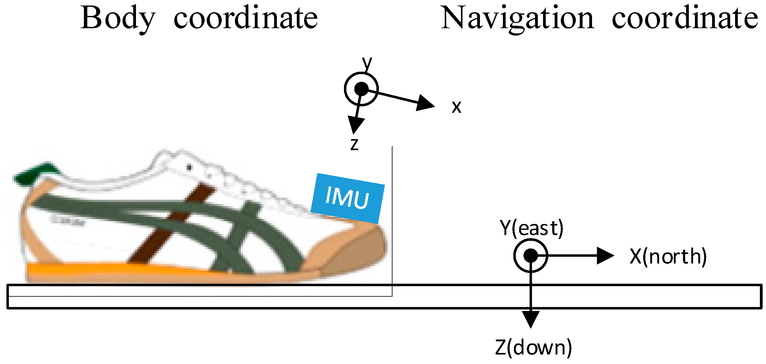
The basic idea of proposed algorithm is to use an IMU for capturing the movement features of the foot. Different IMU installation modes on the foot create different signal features and ZV periods. To the best of our knowledge, there exist four typical IMU installation modes, namely above the instep, above the toe, under the heel and behind the heel. All of them demand a robust way to accurately detect the ZV period. The key problem is how to reduce the ambiguity at the boundaries of the ZV period. In the experiments, the IMU is mounted on the top of toe (
Figure 2). This installation mode has the following advantages:
The gyroscope measurements in the y axis have a sharp slope at the start of the swing period, which could be easily detected.
The duration of the ZV period is relative long.
The IMU measurements are relative stable in the ZV period at high speed.
Figure 2 shows the IMU installation mode and the relationship between body coordinates and navigation coordinates. The following content is analyzed according to this installation mode.
Figure 2.
IMU installation mode and the relationship between body coordinate and navigation coordinate.
Figure 2.
IMU installation mode and the relationship between body coordinate and navigation coordinate.
2.1. Kinesiology Model Analysis
In order to detect the ZV period in the gait cycle precisely, knowledge of the gait during ambulation is introduced as basic theory. The main content is as follows:
Gait cycle: a fundamental unit to describe the gait during ambulation, which occurs from the time when the heel of one foot strikes the ground to the time at which the same foot contacts the ground again.
Heel strike: a heel strike of the same foot.
A typical gait cycle lasts for 1–2 s.
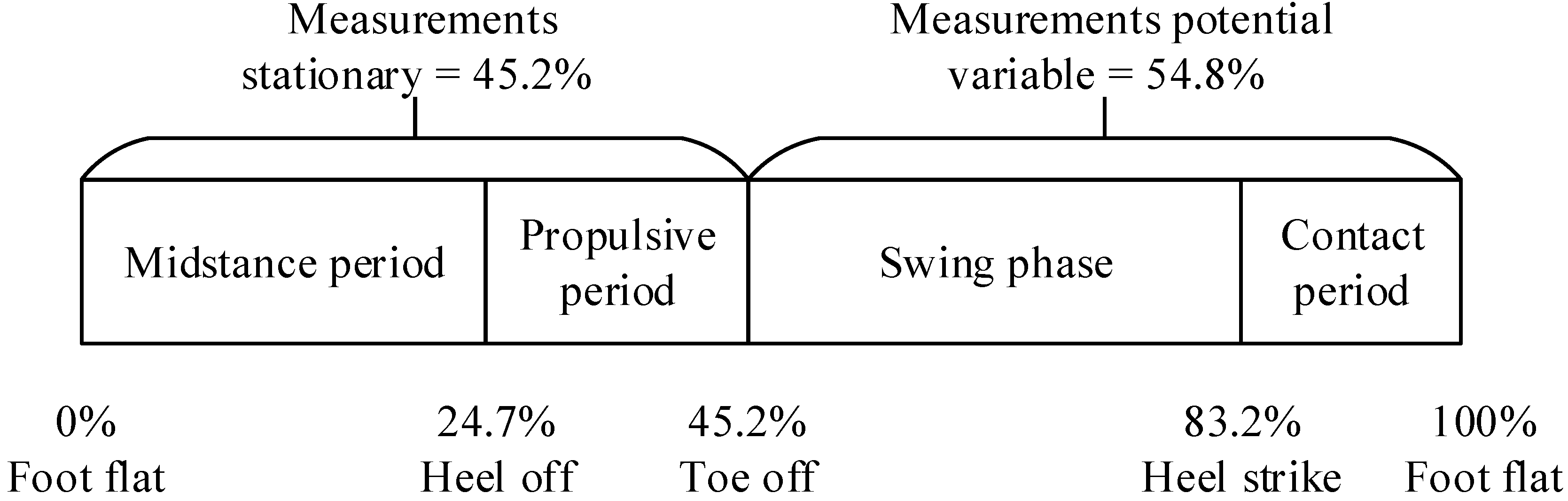
According to the kinesiology knowledge, a whole gait cycle consists of the stance phase and swing phase [
21] (
Figure 3). Moreover, the stance phase includes contact period, midstance period and propulsive period. The IMU signal feature is stationary during the midstance period and propulsive period, but variable during the contact period and swing period. The experiments show that the features of
y axis gyroscope measurements could be used to segment the gait cycle easily and distinguish the start point of a gait. The gait timespan detector is discussed as follows.
Figure 3.
Phases in a typical gait cycle.
Figure 3.
Phases in a typical gait cycle.
2.2. Gait Timespan Calculation
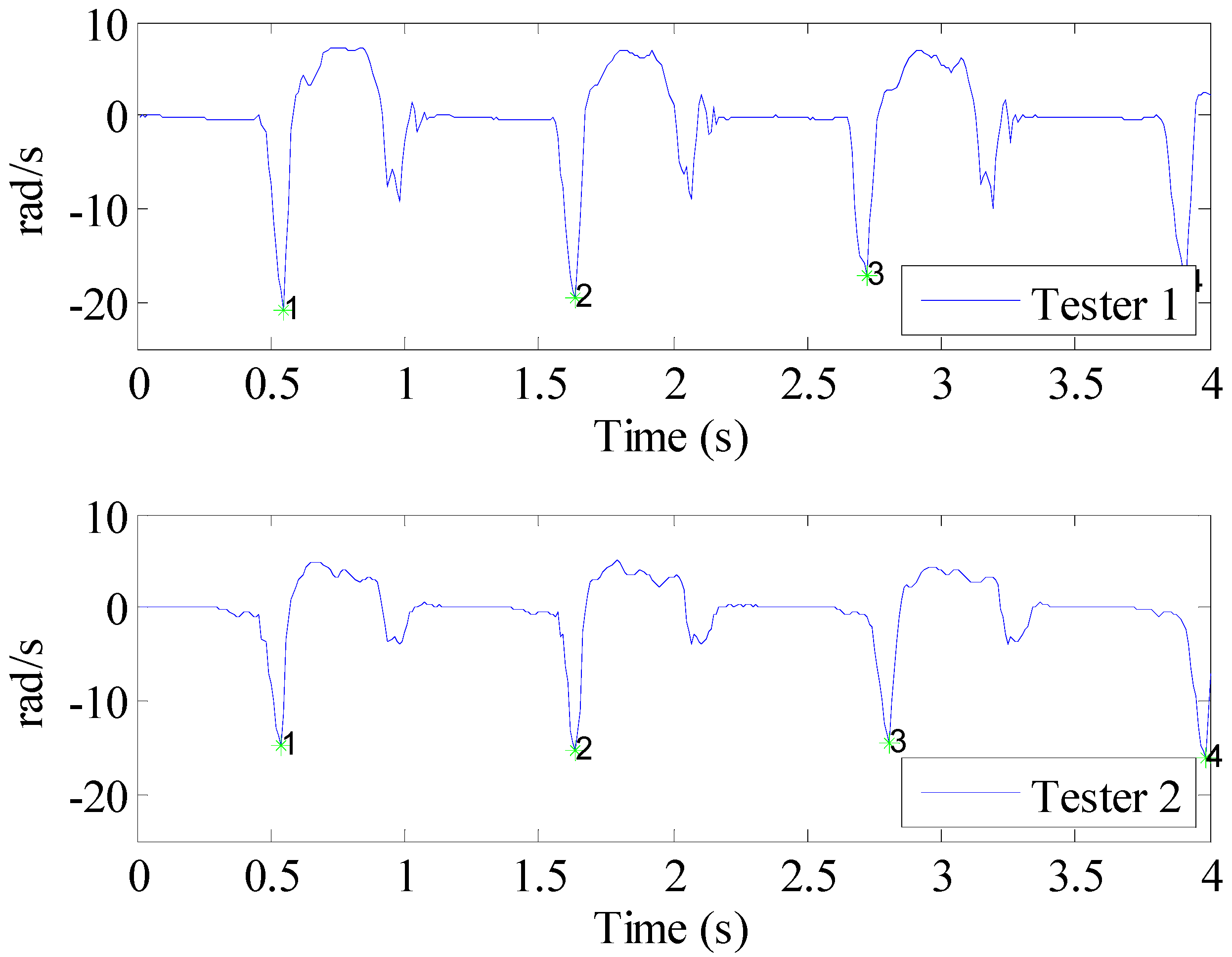
In order to design a robust method to calculate gait timespan, the features of IMU measurements should be analyzed first. The proposed solution is based on y axis gyroscope measurements which have a sharp feature at the start of swing phase.
Figure 4 shows two typical signal types of testers. The upper subplot shows two valleys in one gait cycle, while in the lower subplot, only one valley could be found with same valley detection algorithm. However, the results of two subplots both show that the same valley could always be found at the beginning of swing period. This valley could be used to calculate the duration of one gait. The details are described as follows:
Figure 4.
The y axis gyroscope measurements of two testers.
Figure 4.
The y axis gyroscope measurements of two testers.
The well-known zero-derivative method is used to find the valley. Due to the measurement noise or different walking modes, accidental zero-crossings will occur, so some effective means must be adopted based on the signal features of the y axis angular rate. Once the first valley is found, a delay time will be applied to ignore all the other valleys found during this time. This time span is defined according to kinesiology knowledge as:
where
is the last gait timespan calculated, 0.548 is the proportion of swing phase and contact period in one gait (
Figure 3). Furthermore, a flag is maintained to identify whether the current time instant is in the ZV period. Once the first valley in swing phase is found, the flag is set as false, and if last several samples are ZV, the flag is set as true. When the flag is false, all the other valleys found will also be ignored.
In general, no matter which installation mode is applied, it is inevitable to overcome the ambiguity of the ZV boundary in the contact period. During that short moment, the relative motion between the IMU and foot will create more noise, because the foot strikes the ground. This noise will expand the altitude error, hence, an accurate ZV detector could correct the altitude error better. Based on the kinesiology knowledge and the calculated gait timespan, a data fusion method could be used to reduce the ambiguity of the ZV boundary.
5. Implementation and Evaluation
Several tests have been performed to evaluate the performance of the algorithm. The application framework comprises an Android phone and an IMU with a Bluetooth module which is used to transfer the raw data to the Android unit (
Figure 1). The IMU has 3-axis accelerometers and 3-axis gyroscopes. The choice of dynamic range of the IMU should balance the measurement resolution and the application demands. A wider dynamic range could provide more accurate altitude estimation [
10], but sacrifice resolution. Moreover, the experiments show that the acceleration will exceed 80 m/s
2 when running, so integrated analysis suggests that the range of the accelerometer should be set between
m/s
2. Similarly, the gyroscope is set between
deg/s. The sampling rate is set as 100 Hz, considering the computing resources of the Android platform.
The experiments are executed by different people indoors and outdoors. The scenarios include a floor with multiple rooms, multiple layers and outdoors. Since this application is mainly used in emergency rescue situations, ten physically fit volunteers with ages ranging from 20 to 35 took part in the experiments.
In this section, the proposed method is evaluated in two aspects. Firstly, the proposed ZV method is evaluated. The comparisons of ZV boundary and ZV false detections detected by different methods are shown. Secondly, the 3D Tracking Effect is evaluated. The volunteers travel different close paths to evaluate the horizontal error and upstairs to evaluate the vertical errors.
5.1. ZV Detector Evaluation
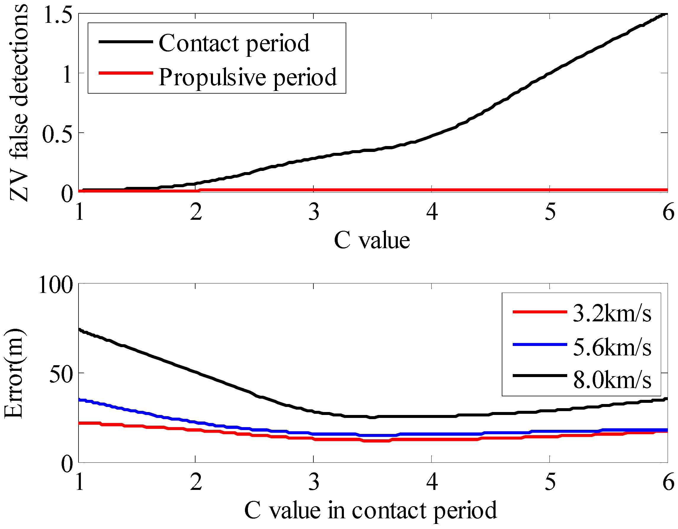
Firstly, In order to verify the Formula (11), the experiments analyzed the average ZV false detections in the contact period and propulsive period with different C values. The data is sampled at a speed of 5.6 km/h. The 1st subplot of
Figure 9 shows that there exists more noise in the contact period. With the increase of C value, more false detections will occur. However, in the propulsive period, the signal feature has a sharp slope, so the number of false detections is small. This means that the C value in the propulsive period has a negligible effect on the algorithm. Thus, the experiment concentrates on the C value in the contact period. The 2nd subplot of
Figure 9 shows the position error with different C values in the contact period.
Figure 9.
The average ZV detections in the contact period and propulsive period with different C values in Formula (11) and horizontal position errors with different C values in the contact period.
Figure 9.
The average ZV detections in the contact period and propulsive period with different C values in Formula (11) and horizontal position errors with different C values in the contact period.
The experiment is performed over a 1 km rectangular closed path. According to the results, a small C value means that the probability distribution of is steep, which will overlook the impact of . However, a large C value suggests that the BN ZV detector will degenerate into the combined condition method. The results show that the C value could be set as 3.5.
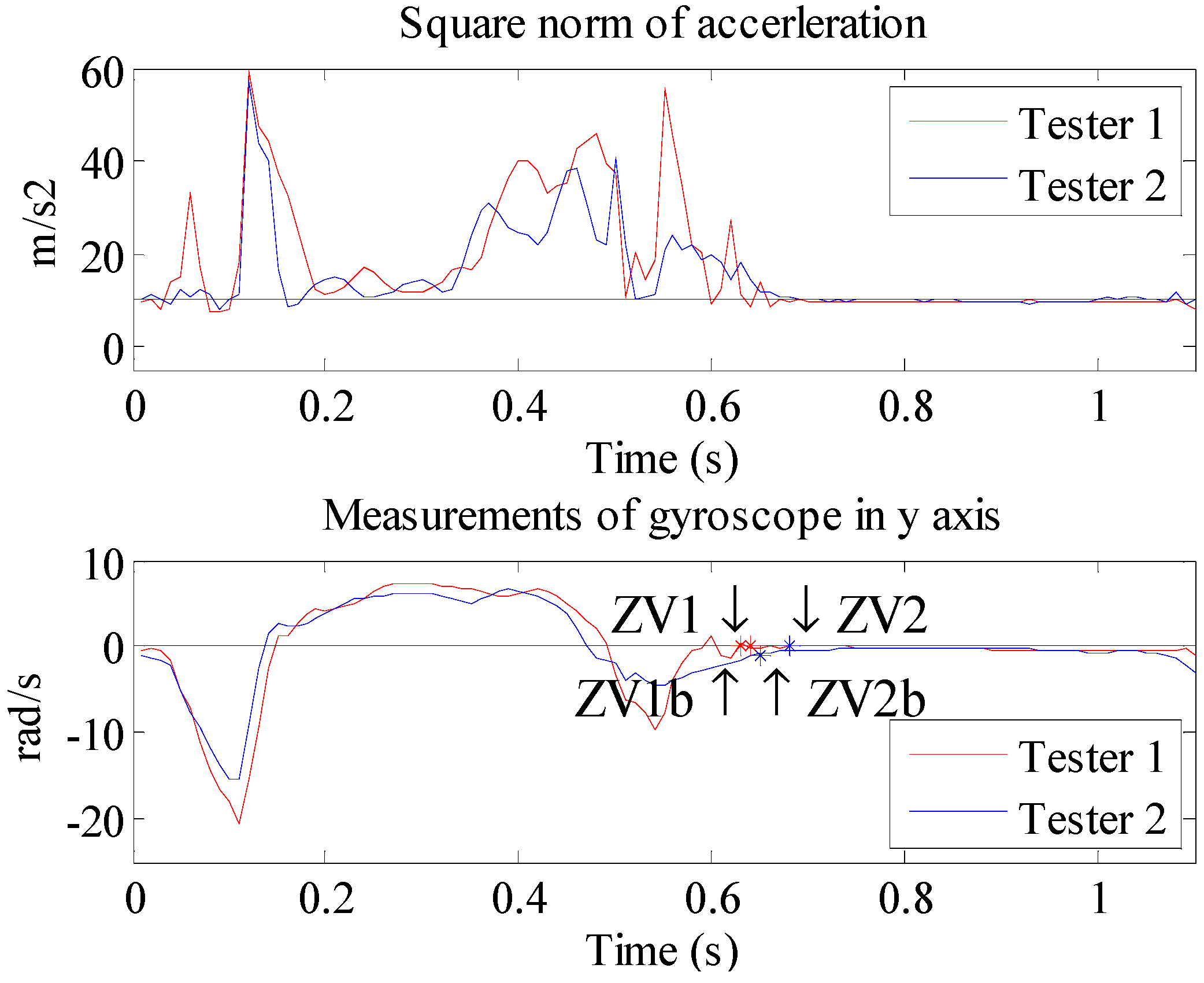
The comparison of the detected ZV boundary between the proposed method and the combined condition method is shown in
Figure 10. Based on the data of two testers, the results suggest that the start of the ZV period determined by the proposed method is 0.01 s (from ZV1 to ZV1b) and 0.04 s (from ZV2 to ZV2b) earlier than the combined condition method, respectively. This is because the foot strikes the ground at the end of the contact period. During this process, more noise is created, which will cause the start time of the ZV period delay detected by the threshold method. Unfortunately, during this short delay time, the position error could increase rapidly.
Figure 10.
The square norm of acceleration and the gyroscope measurements in the y axis of two testers, and the comparison of ZV boundaries obtained by two methods
Figure 10.
The square norm of acceleration and the gyroscope measurements in the y axis of two testers, and the comparison of ZV boundaries obtained by two methods
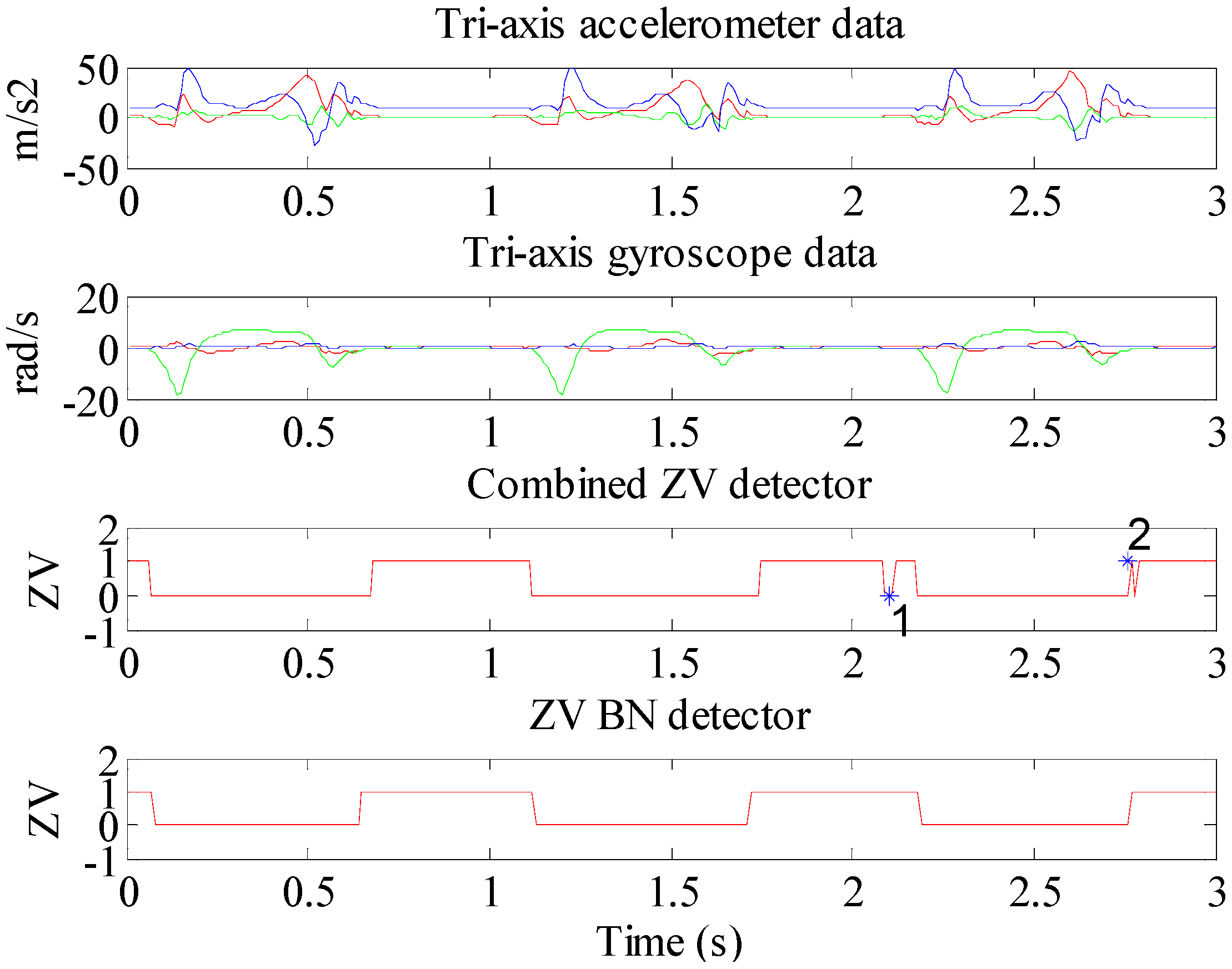
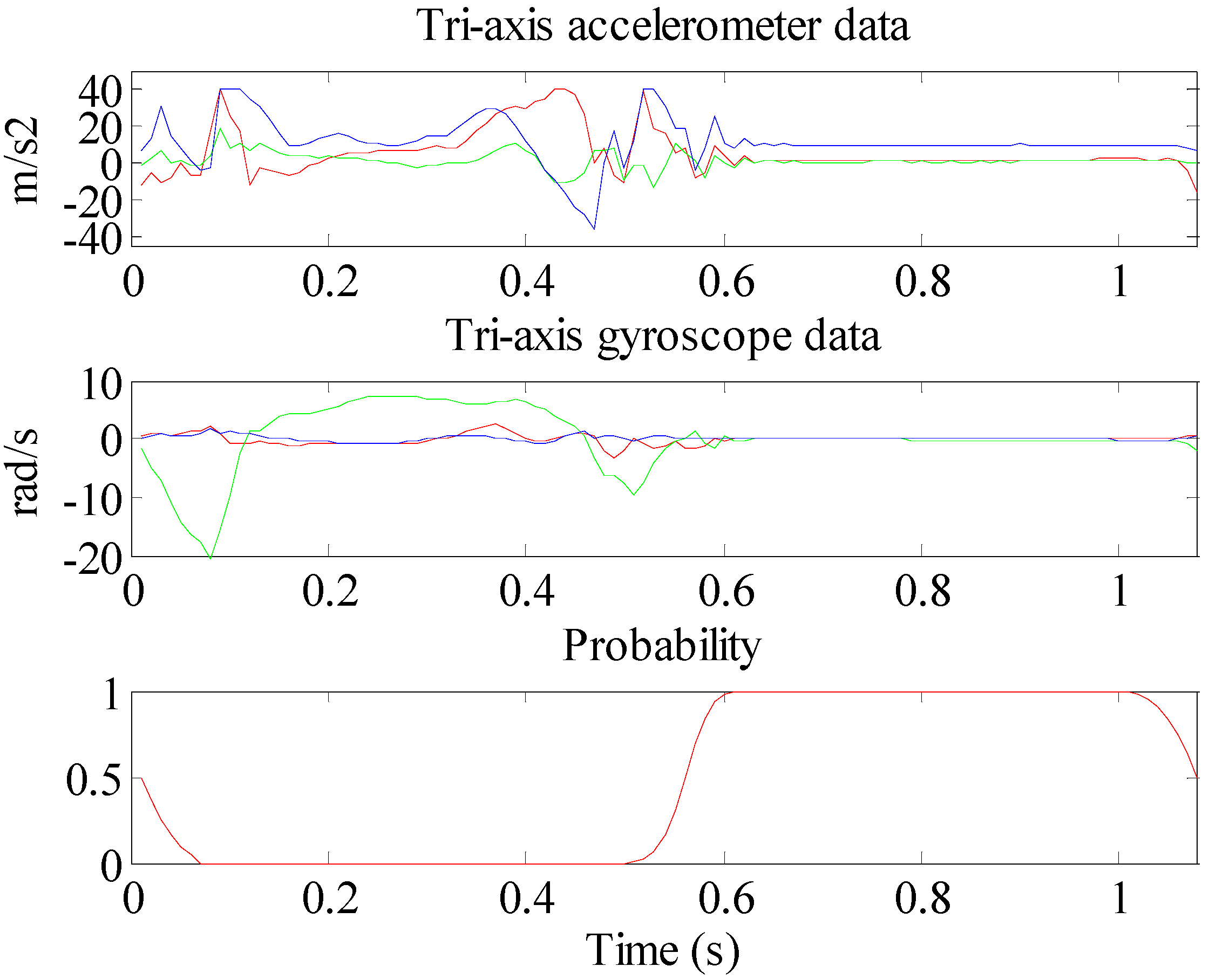
In
Figure 11, the top two subplots are the tri-axis accelerometer and tri-axis gyroscope measurements, respectively. The 3rd subplot is the ZV detected by the combined condition method with median filter, it should be noted that there still exist two ZV false detections, especially point 1 that occurs in the midstance period, which is impossible in practice. Point 2 is an ambiguous detection. The 4th subplot is the ZV result of the proposed method. This ZV result is clearer.
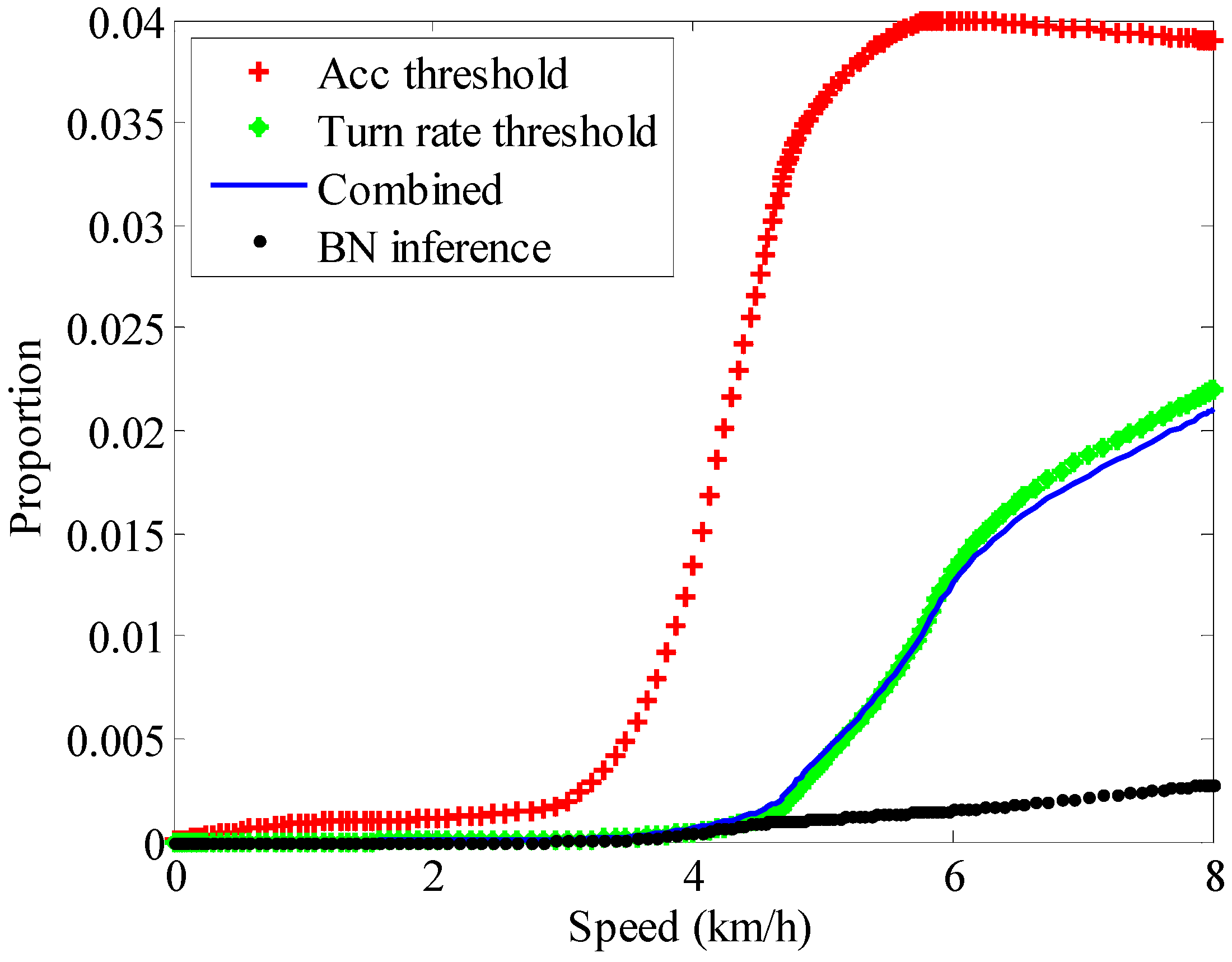
Through the experiments,
Figure 12 shows the proportion of ZV false detections in the total test duration with different methods at different speeds. The experiments are performed at different speed of 1.8, 3.6, 5.6 and 8.0 km/h, respectively. It reveals that the combined method could work well during low speed movement, but when the speed increases, more noise will reduce the accuracy of the algorithm. Some researchers advise that the only angular rate threshold method can provide a relatively stable ZV detector, but in the test, it still could not achieve good performance at high walking speed. Most false detections occur during the transition from the contact period to the midstance period, while the BN inference method could use kinesiology knowledge to reduce the fuzziness of the ZV period to some extent. In short, with the increase of speed, the number of false detections will grow by all the methods, but the BN inference method could limit this growth effectively.
Figure 11.
The comparison of ZV false detections between the combined condition method and the BN inference method.
Figure 11.
The comparison of ZV false detections between the combined condition method and the BN inference method.
Figure 12.
The proportion of ZV false detections in the total test duration with different methods at different speeds.
Figure 12.
The proportion of ZV false detections in the total test duration with different methods at different speeds.
The proportion of detected ZV periods in one gait cycle obtained with different methods has been compared in
Table 1. When the walking speed increases, more noise will occur. This is the reason why the dynamic range of the proportion by the combined condition method is wide. The range of the proposed method is more stable than the method under the combined conditions. On the other hand, when people are running, there exists only very tiny ZV period in one gait cycle based on the combined method, which will fail to locate pedestrians.
Table 1.
The proportion of detected ZV period in one gait cycle by two methods.
Table 1.
The proportion of detected ZV period in one gait cycle by two methods.
| Method | Combined Method (%) | Bayesian Network Inference (%) |
|---|
| ZV in one gait | 18–46 | 32–47 |
5.2. 3D Tracking Effect Evaluation
To evaluate the altitude accuracy of PINS based on the proposed ZV detector, experiments are performed on a horizontal floor. The accuracy of altitude is a tough problem in 3D tracking, because it is constrained for many reasons, including the dynamic range of the accelerometers, accelerometer sensor errors and the accuracy of the ZV detector,
etc. The experiment reveals that the proposed method could improve the altitude accuracy, and reduce the altitude error by 40% on average (
Figure 13).
Figure 13.
Experiment results of altitude error in a total distance of 100 m with ten testers at normal speed.
Figure 13.
Experiment results of altitude error in a total distance of 100 m with ten testers at normal speed.
The entire system is tested in different scenarios.
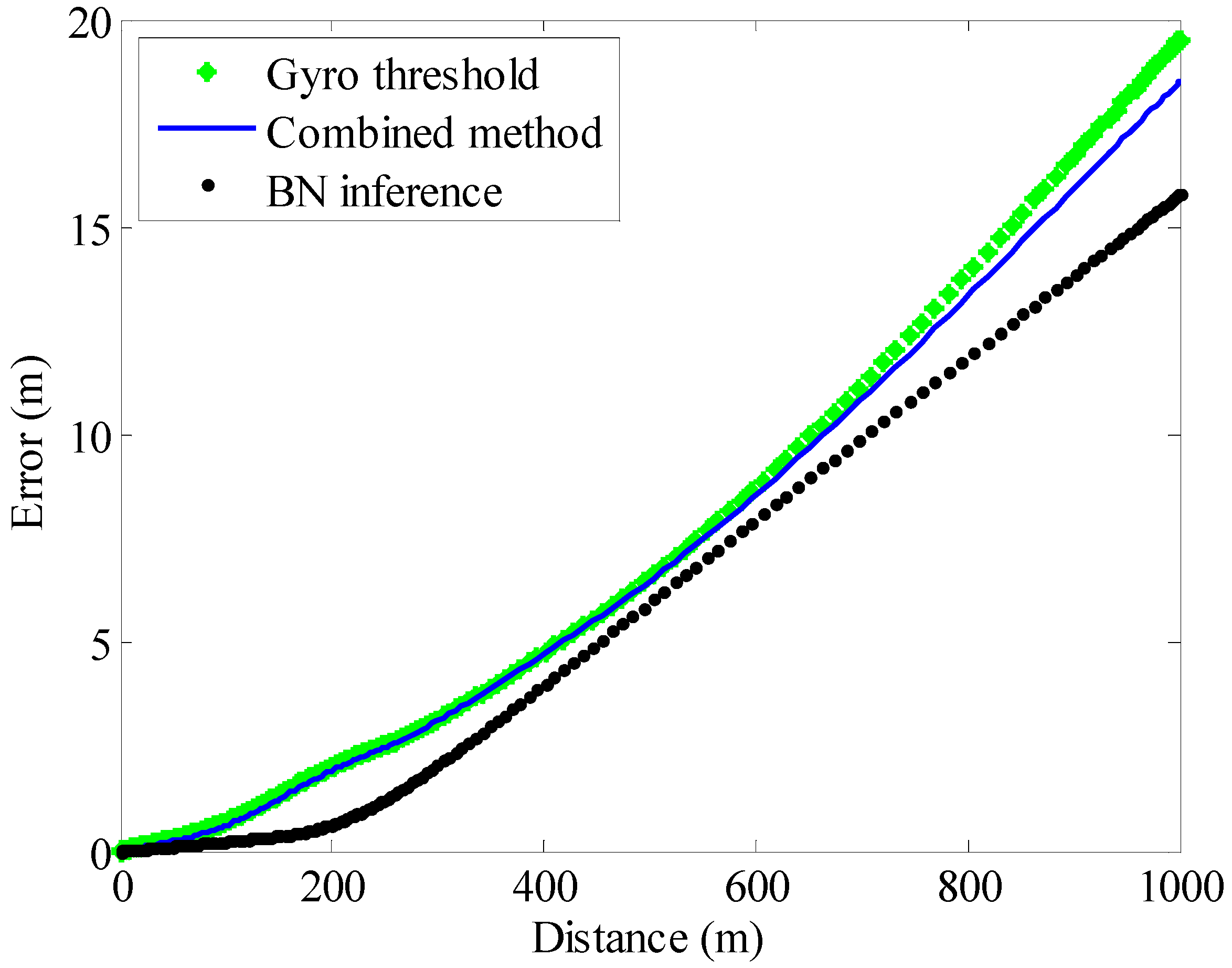
Figure 14 shows the average horizontal errors in the EKF/PINS algorithm based on different ZV detectors. The experiments are performed along a closed path at normal speed (5.6 km/h), and the difference between the start and end points is treated as the horizontal error. The tests’ rectangular paths are 100, 200, 300, 600 and 1000 m in length. The results show that the position error roughly increases linearly with distance, and the proposed ZV detector could also improve the tracking effect.
Figure 14.
Average horizontal error by PINS/EKF based on different ZV detectors.
Figure 14.
Average horizontal error by PINS/EKF based on different ZV detectors.
The experiments prove that the proposed method could compensate the altitude error better (
Figure 15b,d). Meanwhile, an accurate ZV detector could also achieve better horizontal tracking effects. In
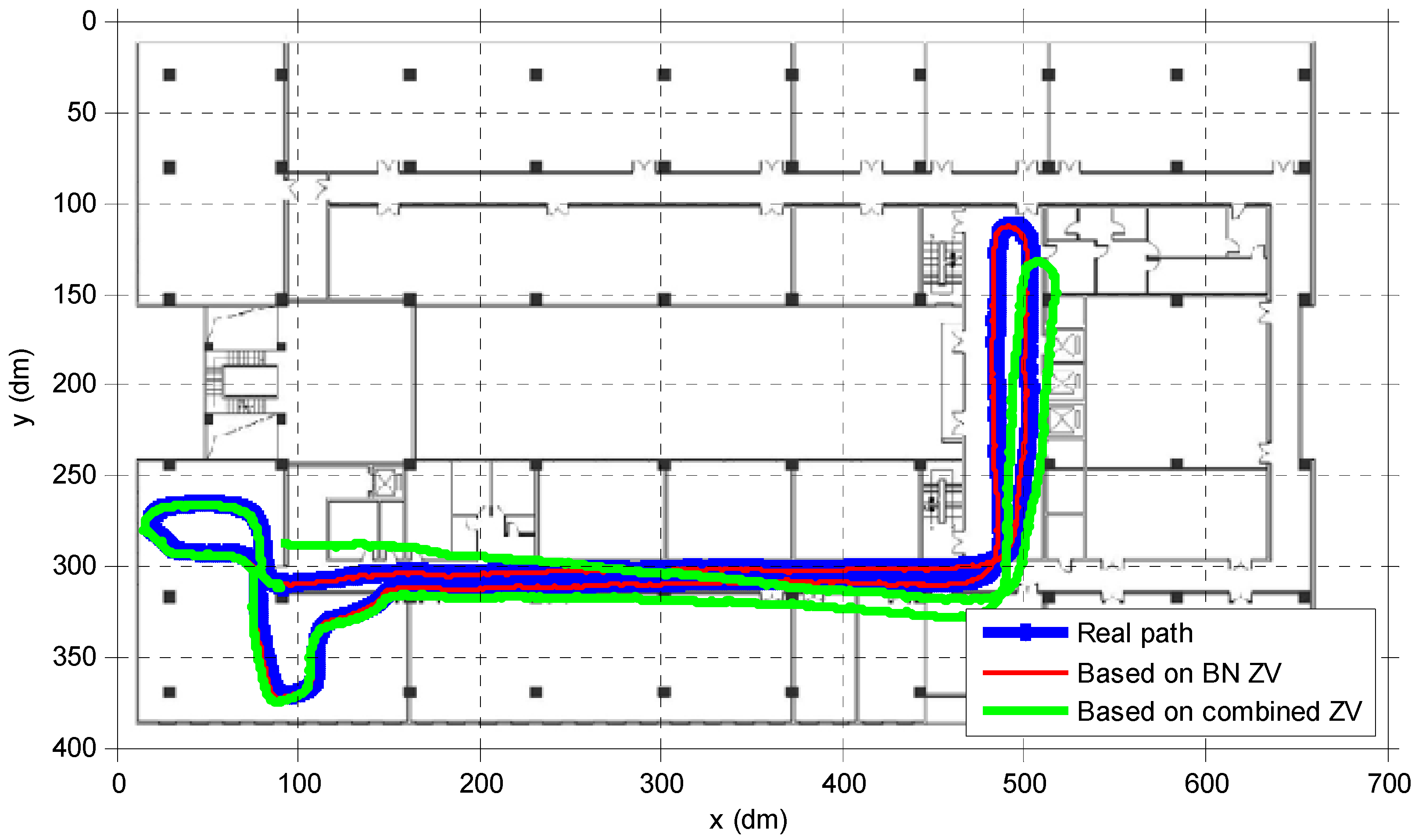
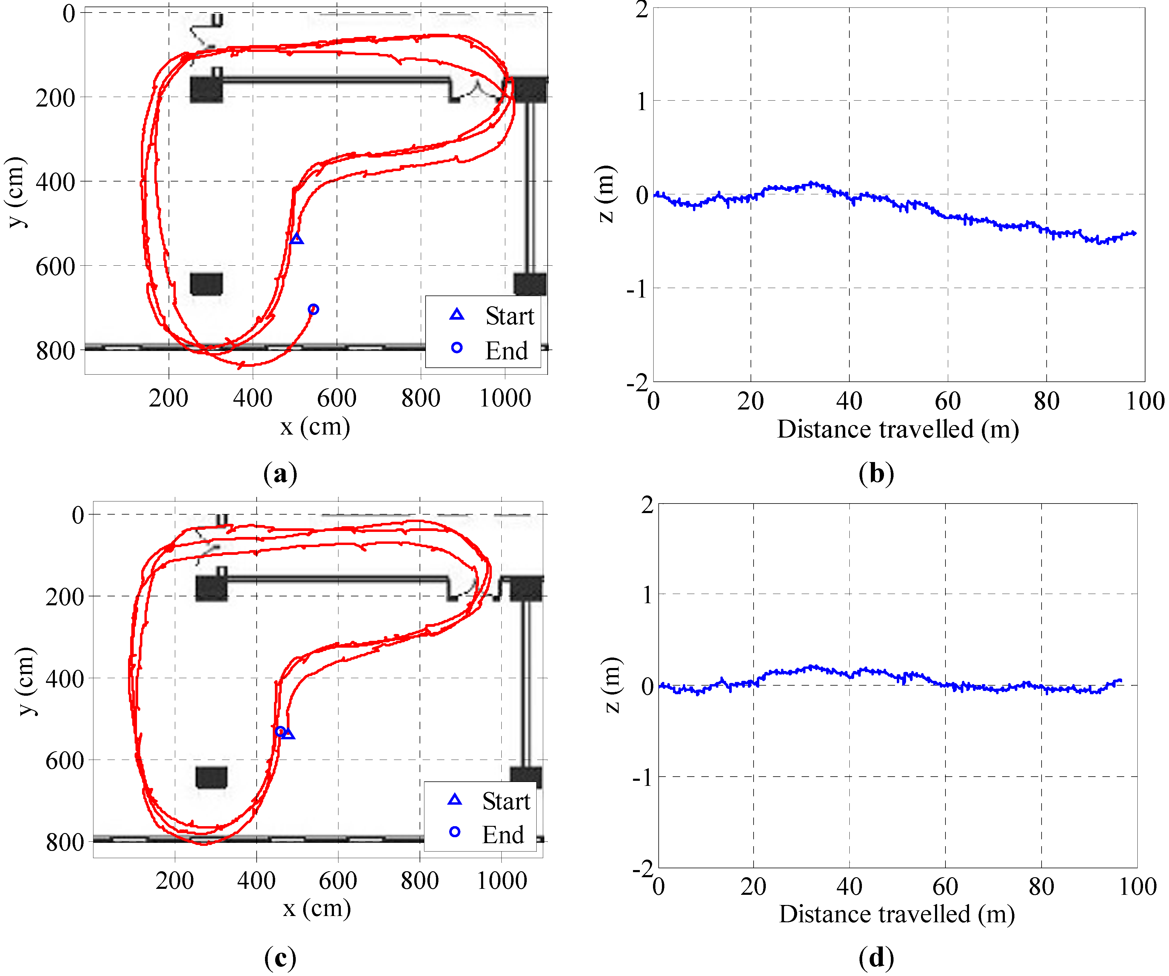
Figure 16, the blue closed path is the real walking path. With the same EKF parameters, the red path based on ZV detector by BN inference method could fit the real path well, while based on the combined condition ZV detector, the green tracking path deviates from the real path.
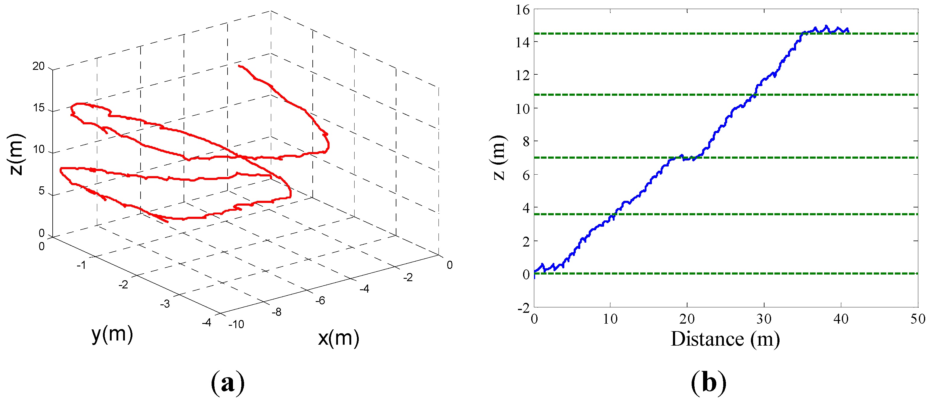
Figure 17 shows the 3D map and altitude map of going upstairs, the result shows a good altitude tracking effect by the EKF/PINS based on the ZV period detected by the BN inference method.
Figure 15.
The comparison of the tracking results based on different ZV detectors. (a) Estimated 2D path based on the combined condition method; (b) Estimated altitude based on the combined condition method; (c) Estimated 2D path based on the BN method; (d) Estimated altitude based on the BN method.
Figure 16.
Estimated indoor 2D path.
Figure 16.
Estimated indoor 2D path.
Figure 17.
(a) Estimated 3D path for going upstairs; (b) Estimated altitude.
Figure 17.
(a) Estimated 3D path for going upstairs; (b) Estimated altitude.
The proposed method to detect the ZV period is robust. To get a better position effect, it is essential to adjust the EKF parameters based on sensor characteristics and the different movement patterns. The experiments show that a different R value in EKF will affect the result. Intuitively, the increase of R will lead to over-steering, and vice versa. This is because when R is big, namely the uncertainty of velocity and angular rate is big, and then the EKF will compensate more. However, the influence of R value on the result is limited because the EKF will converge. In the future, some landmarks could be used to decide whether the tracking is over-steering or under-steering, and adjust R value adaptively. On the other hand, more aided information can be introduced to calibrate the position errors, like maps, RF markers and so on.


