A Simultaneously Calibration Approach for Installation and Attitude Errors of an INS/GPS/LDS Target Tracker

Abstract

To obtain the absolute position of a target is one of the basic topics for non-cooperated target tracking problems. In this paper, we present a simultaneously calibration method for an Inertial navigation system (INS)/Global position system (GPS)/Laser distance scanner (LDS) integrated system based target positioning approach. The INS/GPS integrated system provides the attitude and position of observer, and LDS offers the distance between the observer and the target. The two most significant errors are taken into jointly consideration and analyzed: (1) the attitude measure error of INS/GPS; (2) the installation error between INS/GPS and LDS subsystems. Consequently, a INS/GPS/LDS based target positioning approach considering these two errors is proposed. In order to improve the performance of this approach, a novel calibration method is designed to simultaneously estimate and compensate these two main errors. Finally, simulations are conducted to access the performance of the proposed target positioning approach and the designed simultaneously calibration method.

1. Introduction

To measure the three-dimensional (3D) position of a target in motion is one of the basic problems of target tracking. In this section, we will briefly review the sensors commonly used for measuring the position of a target. Consequently, an Inertial navigation system (INS)/Global position system (GPS)/Laser distance scanner (LDS) integrated system based target positioning approach is introduced.

1.1. Sensors for Target Tracking

Target tracking [1] by using different sensors is a significant field of work for the application areas of military applications [2,3], pedestrians surveillance [4,5] and autonomous robotics [6,7]. Most existing research work on target tracking concentrates on efficient ways of modeling [8,9] and trajectory estimation methods [10,11], as well as on varieties of data association approaches[12,13], which are extremely significant for the multiple target tracking problem [14,15].

However, there is comparatively less work that refers to the sensors in target tracking. Meanwhile, only a little of the literature is concerned about the low-cost target tracking field. For the demonstration of a 3D object’s motion, the parameters related to the linear motion and rotation is extremely essential information.

For the tracking problem of cooperated targets, generally almost all the navigation systems and their sensors are efficient information sources, such as INS, GPS and celestial navigation system. These traditional navigators based on different positioning principles could supply the 3D position. However, it is necessary to mount these navigators and sensors on the targets, which is practically impossible when tracking a non-cooperative target.

For the sensors commonly used in target tracking, we put forward a summary as follows. In this summary, some special sensitive sensors are not included, such as the gravity instrument and magnetometer.

(1)

Radar [16,17]—which might be the most predominant sensor in this field, and its advanced developments, such as the monostatic radar and multistatic radar (bistatic radar, multi-input and multi-output radar [18]). A radar exhibits excellent performance for detection and feedback measurements, not only the range information of targets but also their bearings.

(2)

IR sensor [19–21]—which is often used to detect and locate the infra-red emit object by visual, or performs as a thermal imaging system to provide a radiant temperature distribution graph. Individually or as an assisted subsystem, the IR sensor has be widely used in military applications, such as the airplane forward/side looking system [22] and the detector for smart attack munition.

(3)

Electronic-optic sensor [23–25]—which is used for the both-way converts between light and electronic signals, typically the camera.

(4)

Electronic support measurement [15]—could only provide angular measurements, and usually passively detecting the radar signals delivered by targets.

(5)

Laser sensor [26,27]—which is ideal for the non-contact measurement of range, with a long effective range. A detection method based on the laser scanner could obtain the 3D position of the surface of objects by laser distance detecting. However, the obtained 3D position are the information the object corresponding to the instrument coordinates.

(6)

Acoustic sensor [28,29]—which could convert the physical acoustic signals into digital signals, specially suitable for the underwater vehicle detection and tracking, despite easily be influenced by environment noise. Sonar is a common one for this kind sensor.

(7)

Sensor network [30,31]—which commonly utilize multiple or even multiclass low-accuracy and cheap sensors to efficiently tracking for randomly appearing objects. Their effective range is usually small, and they are frequently used in the indoor or local area surveillance. Wireless sensor network [28] are developed to extend the range as well as reduce the complex of physical network connection.

(8)

Binary proximity sensor [32,33]—which is low-cost and economical for the computation complexity for only provide binary detection, usually combined to form sensor network.

1.2. INS/GPS/LDS System Based 3D Positioning Approach

The mapping principle of 3D laser scanner [27], which is quite similar to that of the optical theodolite and the total station device, is based on the characteristic of straight propagation of the light. The only difference is that 3D laser scanner has one more function that could measure the distance between the device and its target.

By this mapping method, we could obtain the 3D coordinates of the point at the surface of target, and then quickly establish a 3D model of the object. However, this method has a disadvantage that the obtained coordinates of the points are related to the measurement coordinate system [34]. In [35], a method is designed for target navigation and mapping based on the INS/GPS/LDS integrated system, in which inertial sensors are utilized to provide the rotation measurements to map the range information in the measurement coordinate system into that in the geographic coordinate. The impact of the attitude errors of inertial sensors on the mapping performance are consequently investigated and calibrated. With a high-frequency update, this method could be used for target tracking. However, the work of [35] is based on an assumption that all the three subsystems are precisely installed. Before the real application, the misalignment error between the sensitive axes of INS/GPS system and LDS should be compensated to be minimum, to avoid an over large positioning error.

Suffering from the limits of machining and the measurement error of devices, there are non-orthogonal coordinate systems that exist in the INS/GPS/LDS system:

(1)

the non-orthogonal coordinate of inertial sensors;

(2)

the non-orthogonal coordinate between LDS and INS/GPS system.

To guarantee the accuracy of measurement, calibration is needed to transform the non-orthogonal coordinates into the orthogonal ones. For instance, for a INS/GPS integrated system, the transformation can be realized by conducting the calibration by using a three-axle rotational table in the laboratory [36,37]. As for the laser scanner, [38,39] give some suitable calibration schemes. However, the content of calibration for the misalignment between INS/GPS and LDS is almost blank for the different measurement principles of these two systems. Advanced physical machining and precisely installation seem like available solutions, but undoubtedly they will lead to the problem of high cost and strict demands for the machining technology.

In this paper, we present an error calibration method for an INS/GPS/LDS tracker, to jointly estimate and compensate the installation and attitude errors. In Section 2, the target positioning method based on INS/GPS/LDS is analyzed and then a modified target mapping approach by considering the installation error between INS/GPS and LDS subsystems is presented. In Section 3, the target positioning error of this approach is investigated by taking the installation error into consideration. Furthermore, we address the corresponding calibration algorithm in Section 4, in which external reference points are introduced and their information are adopted to synchronously calibrate both the installation error and the attitude measurement error of INS/GPS system. Finally, simulations are conducted to verify the validity of the calibration algorithm and the positioning performance of the entire system.

2. Algorithm Description for Calculating the Position of Target

2.1. The Conventional INS/GPS/LDS System Based Approach

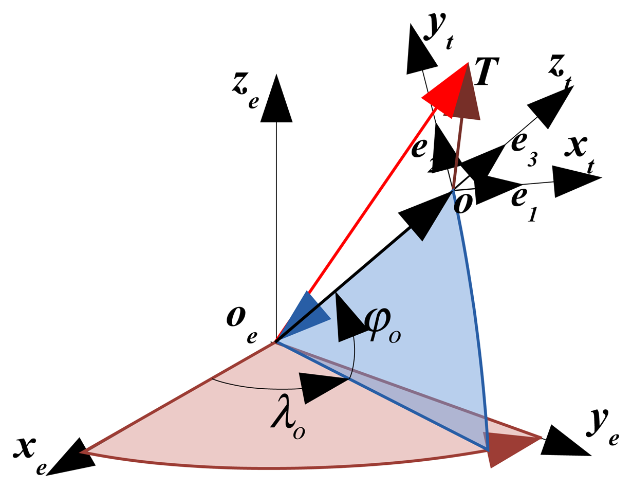
For the convenience of calculating the target coordinate with the conventional INS/GPS/LDS system based method, a vector of oT defined between the observation point o to the target T is introduced. The mathematical representation of oT is related with distance d, yaw H and pitch ϕ (the angles are defined in the local geographic coordinate system) between o and T. In order to calculate the absolute coordinate of T, the vector oT should be converted into a corresponding vector within the earth coordinate system. In this convert, the necessary information we needed includes: (a) the position information of the target T, which has been measured in the local geography coordinate system; (b) the position of the observation point o in the earth coordinate system. Figure 1 shows the target T in the geographic ox_ty_tz_t and earth coordinate system ox_ey_ez_e.

The basic procedure of the INS/GPS/LDS based approach are

(1)

Definition of the basis vector oC in ox_ty_tz_t

In order to demonstrate oT by using the attitudes defined in ox_ty_tz_t, which are measured by INS/GPS subsystem, a basis vector of oC is defined along the oy_t axis of ox_ty_tz_t. The vector is described as

$$\mathbf{\text{oC}}=0{\text{e}}_1+d{\text{e}}_2+0{\text{e}}_3$$

(1)

where, e₁, e₂, e₃ are the unit vectors along the three axes of ox_ty_tz_t, respectively; and d is the distance between o and T.

(2)

Describe the vector of oT in ox_ty_tz_t

The measure principle of LDS guarantee its sensitive axis would have the same direction with the vector of oT. Therefore, we assume that the direction of oT is along with the oy_b axis of the body coordinate system ox_by_bz_b. The vector oT can obtained from oC after twice rotations with the angles of H and ϕ, respectively. The rotations can be expressed by the direction cosine matrix as

$${\mathbf{\text{C}}}_t^b=\left[\begin{array}{ccc}1& 0& 0\\ 0& cos\varphi & sin\varphi \\ 0& -sin\varphi & cos\varphi \end{array}\right]\cdot \left[\begin{array}{ccc}cosH& sinH& 0\\ -sinH& cosH& 0\\ 0& 0& 1\end{array}\right]$$

(2)

where, ϕ and H denote the pitch and yaw, respectively. The angles and the transform matrix ${\mathbf{\text{C}}}_t^b$ are used to describe the twice rotation relationship between the geographic ox_ty_tz_t and the body coordinate system ox_by_bz_b, where is the platform LDS placed. Then, the vector oT can be described in the geographic coordinate system:

$$\mathbf{\text{oT}}={\mathbf{\text{C}}}_t^b\cdot \mathbf{\text{oC}}$$

(3)

The 3D coordinate of o in ox_ty_tz_t can be obtained by combining Equations (2) and (3) as follows.

$$\left[\begin{array}{l}{x}_{oT}^t\hfill \\ y_{oT}^t\hfill \\ z_{oT}^t\hfill \end{array}\right]=\left[\begin{array}{ccc}1& 0& 0\\ 0& cos\varphi & sin\varphi \\ 0& -sin\varphi & cos\varphi \end{array}\right]\cdot \left[\begin{array}{ccc}cosH& sinH& 0\\ -sinH& cosH& 0\\ 0& 0& 1\end{array}\right]\cdot \left[\begin{array}{c}0\\ d\\ 0\end{array}\right]=\left[\begin{array}{c}dsinH\\ dcos\varphi cosH\\ -dsin\varphi cosH\end{array}\right]$$

(4)

(3)

Describe the vector oT in ox_ey_ez_e

Provided the latitude φ_o and longitude λ_o of the point o, the 3D coordinate of oT after being converted from ox_ty_tz_t to ox_ey_ez_e is

$$\left[\begin{array}{c}{x}_{oT}^e\\ y_{oT}^e\\ z_{oT}^e\end{array}\right]={\mathbf{\text{C}}}_t^e\cdot \left[\begin{array}{c}{x}_{oT}^t\\ y_{oT}^t\\ z_{oT}^t\end{array}\right]$$

(5)

where, ${\mathbf{\text{C}}}_t^e$ is the transform matrix from the geographic coordinate system ox_ty_tz_t to the earth coordinate system ox_ey_ez_e [40], and

$${\mathbf{\text{C}}}_t^e=\left[\begin{array}{ccc}cos{\lambda }_o& -sin{\lambda }_{o}cos{\phi }_o& sin{\lambda }_{o}cos{\phi }_o\\ cos{\lambda }_o& cos{\lambda }_{o}cos{\phi }_o& -cos{\lambda }_{o}sin{\phi }_o\\ 0& sin\phi & cos{\phi }_o\end{array}\right]$$

(6)

As shown in Figure 1, three vectors o_eT, o_eo and oT follow the relationship:

$${\mathbf{\text{o}}}_e\mathbf{\text{T}}={\mathbf{\text{o}}}_e\mathbf{\text{o}}+\mathbf{\text{oT}}$$

(7)

By Equations (5) and (7), the 3D absolute position of target in ox_ey_ez_e can be calculated:

$$\left[\begin{array}{l}{x}_T^e\hfill \\ y_T^e\hfill \\ z_T^e\hfill \end{array}\right]=\left[\begin{array}{l}{x}_o^e\hfill \\ y_o^e\hfill \\ z_o^e\hfill \end{array}\right]+{\mathbf{\text{C}}}_t^e\left[\begin{array}{c}dsinH\\ dcos\varphi sinH\\ -dsin\varphi cosH\end{array}\right]$$

(8)

where, ${\left[x_T^e,y_T^e,z_T^e\right]}^T$ and ${\left[x_o^e,y_o^e,z_o^e\right]}^T$ are the 3D coordinates of target T and the observer point o in the earth coordinate system ox_ey_ez_e, respectively. The geographic coordinate of the observer point (latitude φ_o and longitude λ_o), and the 3D coordinate $\left[x_o^e,y_o^e,z_o^e\right]$, the yaw H, the pitch ϕ can be measured by INS/GPS subsystem, while the distance d between the target and the observer point can be measured by LDS. As seen from Equation (8), it is obvious that the absolute 3D coordinate of the target can be calculated by the measurements of INS/GPS/LDS. In addition, other useful information such as the height difference, incline angle, horizontal angle can also be introduced to assist the calculation.

2.2. Problems Caused by the Initial Installation Error

According to the previous analysis in [35], each part of INS/GPS/LDS integrated system would inevitably have measurement error. Therefore, the actual coordinate should be expressed as:

$$\left[\begin{array}{l}{\tilde{x}}_T^e\hfill \\ {ỹ}_T^e\hfill \\ {\tilde{z}}_T^e\hfill \end{array}\right]=\left[\begin{array}{l}{\tilde{x}}_o^e\hfill \\ {ỹ}_o^e\hfill \\ {\tilde{z}}_o^e\hfill \end{array}\right]+{\mathbf{\text{C}}}_t^e\left[\begin{array}{c}\tilde{d}sin\tilde{H}\\ \tilde{d}cos\tilde{\varphi }sin\tilde{H}\\ -\tilde{d}sin\tilde{\varphi }cos\tilde{H}\end{array}\right]$$

(9)

where, the variables with the superscript “∼” denote that their values contain errors. In [35], among the error sources, the attitude error of INS/GPS dominates the calculation accuracy. By introducing an outer reference point, the yaw error and pitch error of INS/GPS can be precisely estimated and compensated.

However, besides the attitude error, the initial installation error between INS/GPS and LDS subsystems should be also taken into consideration. The sensitive axes of these two systems should be maintained along the same directions, or aligned with the corresponding installation basis. Otherwise, the angle difference between the vectors oT and oC should not be equal to the yaw and pitch outputted by INS/GPS system.

To calibrate the installation error, physical calibration methods are commonly adopted among many engineering applications. However, such kinds of solutions usually demand high-accuracy instruments, which could provide precise reference for installation, leading to over high requirement for machining as well as the cost. Based on the experience of calibration for the attitude error of INS/GPS in [35], soft calibration schemes appear to be more reasonable. It seems also available to estimate both the installation and attitude error by using the information of other reference points, which have been already precisely measured.

2.3. Target Positioning Algorithm by Considering the Installation Error

In the general inertial measurement unit, each gyro and its corresponding accelerometer should be aligned with the same direction. Unfortunately, it is almost impossible to realize that. Consequently, two non-orthogonal coordinate systems are formed, which are consisting of gyroscopes and accelerometers, respectively. Calibration for these installation error and non-orthogonal characteristics is necessary for their effective operation. The two non-orthogonal coordinate systems should be converted into orthogonal coordinate systems [37], which is also needed for the LDS and INS/GPS.

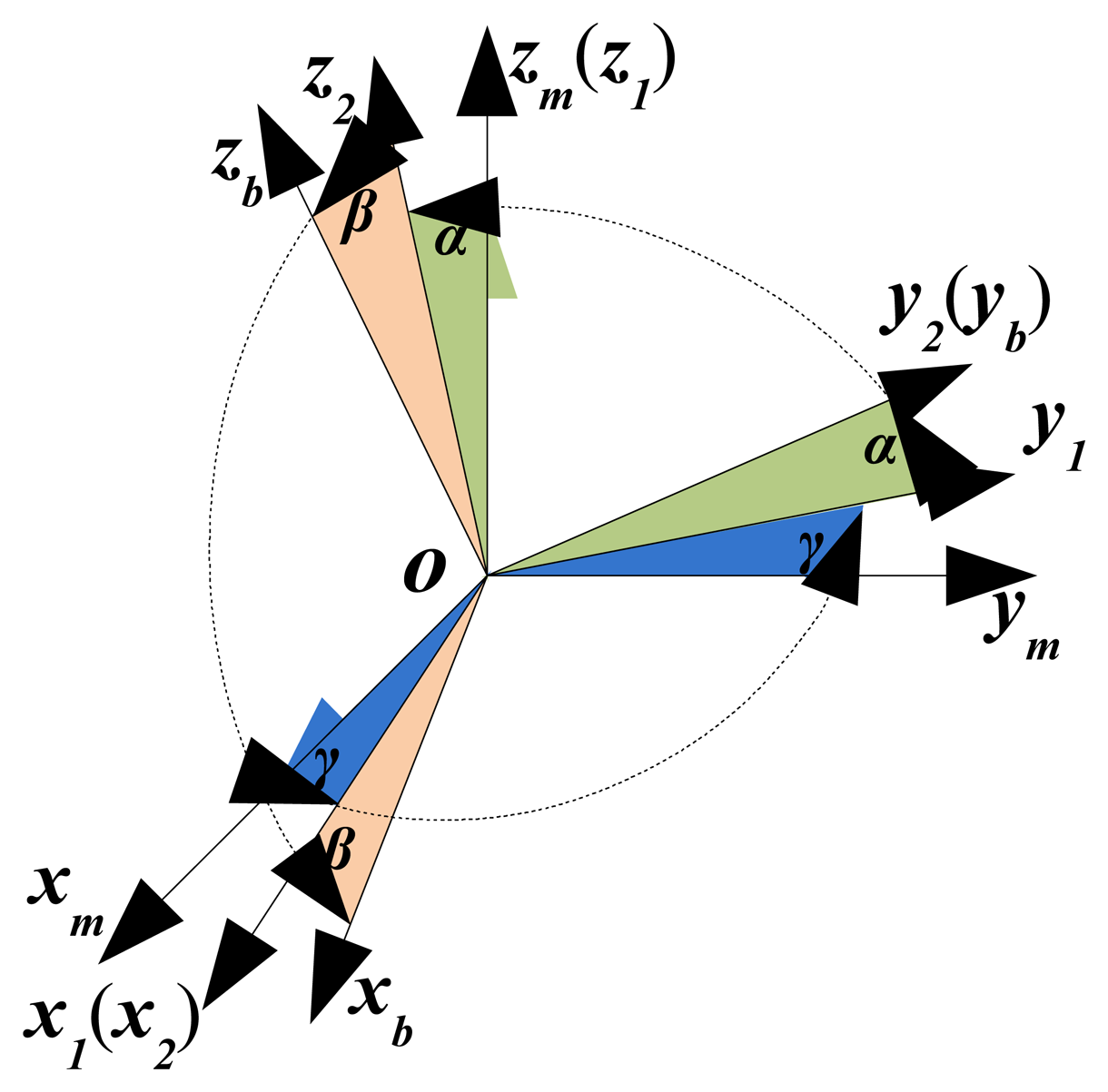
Assuming that the calibrated coordinate system of INS/GPS is ox_my_mz_m, LDS is mounted along the axis of oy_b. There are three misalignment angles α, β and γ between ox_my_mz_m and ox_by_bz_b, which denote the installation error between INS/GPS and LDS subsystems, as shown in Figure 2. Considering the minor angle situation, the transformation matrix between the two coordinate systems of INS/GPS and LDS can be expressed as:

$${\mathbf{\text{C}}}_m^b=\left[\begin{array}{ccc}1& \gamma & -\beta \\ -\gamma & 1& \alpha \\ \beta & -\alpha & 1\end{array}\right]$$

(10)

As can be seen in Figure 2, when the installation error between INS/GPS and LDS exists, the yaw and pitch outputs of INS/GPS are not equal to the rotation angles of oC. The main reason is that only LDS is mounted along the axis oy_b, which is fixed in ox_by_bz_b. However, for the rotation defined in the measurement coordinate system of INS/GPS, the actual rotational angle relates to the axis oy_m .

Define a new vector oC_m, whose mode is d and its direction along with the axis oy_m. Therefore, the vector oC_m can be expressed as

$$\mathbf{\text{o}}{\mathbf{\text{C}}}_m={\mathbf{\text{C}}}_b^m\cdot \mathbf{\text{oC}}$$

(11)

where, ${\mathbf{\text{C}}}_b^m={\left({\mathbf{\text{C}}}_b^m\right)}^T$.

It can be seen from Equation (11) that the rotation described by the attitude measured by INS/GPS can be a vector rotated by oC_m, which could indicate the actual target position impacted by the misalignment angles or installation error.

Substituting Equation (11) into Equation (9), we could obtain:

$$\left[\begin{array}{c}{\tilde{x}}_T^e\\ {ỹ}_T^e\\ {\tilde{z}}_T^e\end{array}\right]=\left[\begin{array}{c}{\tilde{x}}_o^e\\ {ỹ}_o^e\\ {\tilde{z}}_o^e\end{array}\right]+{\mathbf{\text{C}}}_t^e\cdot {\mathbf{\text{C}}}_t^b\left[\begin{array}{ccc}1& \gamma & -\beta \\ -\gamma & 1& \alpha \\ \beta & -\alpha & 1\end{array}\right]\cdot \left[\begin{array}{c}0\\ \tilde{d}\\ 0\end{array}\right]$$

(12)

After simplification, the target positioning algorithm by considering the installation error can be expressed as:

$$\left[\begin{array}{c}{\tilde{x}}_T^e\\ {ỹ}_T^e\\ {\tilde{z}}_T^e\end{array}\right]=\left[\begin{array}{c}{\tilde{x}}_o^e\\ {ỹ}_o^e\\ {\tilde{z}}_o^e\end{array}\right]+{\mathbf{\text{C}}}_t^e\left[\begin{array}{c}\tilde{d}sin\tilde{H}-\gamma \tilde{d}cos\tilde{H}\\ \tilde{d}cos\tilde{\varphi }cos\tilde{H}+\gamma \tilde{d}cos\tilde{\varphi }sin\tilde{H}+\alpha \tilde{d}sin\tilde{\varphi }\\ -\tilde{d}cos\tilde{\varphi }cos\tilde{H}-\gamma \tilde{d}sin\tilde{\varphi }sin\tilde{H}+\alpha \tilde{d}cos\tilde{\varphi }\end{array}\right]$$

(13)

Obviously, the installation error denoted by two misalignment angles of ϕ and γ will directly influence the 3D coordinate’s calculation.

3. Positioning Error Analysis by Considering Installation Error

Under an ideal condition without installation error, a positioning error analysis has been conducted in [35]. As its conclusion, the attitude error of INS/GPS appears to be the most dominant error source. In this section, the extended error analysis about the installation error are implemented.

By ignoring the other errors of INS/GPS and LDS, the positioning error caused by non-ideal installation can be obtained by the minus between Equations (13) and (8), which is given as:.

$${\mathrm{\Delta }}_T=\left[\begin{array}{c}{\tilde{x}}_T^e\\ {ỹ}_T^e\\ {\tilde{z}}_T^e\end{array}\right]-\left[\begin{array}{c}{x}_T^e\\ y_T^e\\ z_T^e\end{array}\right]={\mathbf{\text{C}}}_t^e\left[\begin{array}{c}-\gamma dcosH\\ \gamma dcos\varphi sinH+\alpha dsin\varphi \\ -\gamma dsin\varphi sinH+\alpha dcos\varphi \end{array}\right]$$

(14)

where, ${\mathrm{\Delta }}_T={\left[\mathrm{\Delta }{x}_T^e,\mathrm{\Delta }{y}_T^e,\mathrm{\Delta }{z}_T^e\right]}^T$ is the positioning error caused by the installation error. The matrix of ${\mathbf{\text{C}}}_t^e$ in Equation (14) is an orthogonal matrix, which exhibits the following properties:

$$\{\begin{array}{l}{\left({\mathbf{\text{C}}}_t^e\right)}^{-1}={\left({\mathbf{\text{C}}}_t^e\right)}^T\hfill \\ \left|{\mathbf{\text{C}}}_t^e\right|=1.\hfill \end{array}$$

(15)

The variance of positioning error caused by the installation error can be calculated:

$$\mathrm{\Delta }{P}_T=\sqrt{{\left({\mathrm{\Delta }}_T\right)}^T{\mathrm{\Delta }}_T}=\sqrt{{\left({\mathrm{\Delta }}_{\varphi }\right)}^T\cdot {\left({\mathbf{\text{C}}}_t^e\right)}^T\cdot {\mathrm{\Delta }}_{\varphi }}$$

(16)

where,

$${\mathrm{\Delta }}_{\varphi }=\left[\begin{array}{c}-\gamma dcosH\\ \gamma dcos\varphi sinH+\alpha dsin\varphi \\ -\gamma dsin\varphi sinH+\alpha dcos\varphi \end{array}\right]$$

Substituting Equations (14) and (15) into Equation (16), we obtain

$$\mathrm{\Delta }{P}_T=\sqrt{{\left({\mathrm{\Delta }}_T\right)}^T{\mathrm{\Delta }}_T}=d\cdot \sqrt{{\left(\varphi \right)}^2+{\left(\gamma \right)}^2}$$

(17)

As for Equation (17), the minor error angle condition is taken into consideration. The term $\sqrt{{\left(\varphi \right)}^2+{\left(\gamma \right)}^2}$ denotes their numerical solution.

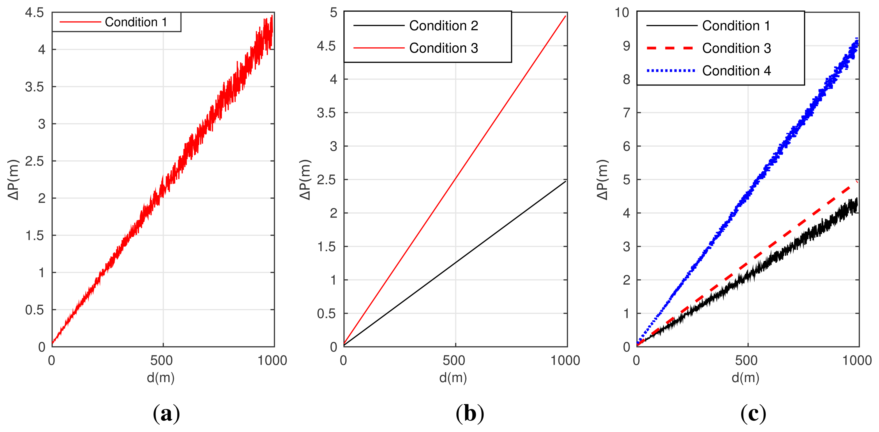
In the following part, simulations are conducted to provide the mathematical explain for the analysis result shown in Equation (17). Assuming the initial position of the point o is obtained (with the longitude 120° and the latitude 45°), and the measure noise for position is 0.2 m; the yaw and pitch error of INS/GPS is 0.2° and 0.1°, respectively. The measure noise of LDS is 5 mm for the target within 300 m, and has an additional linearity error for 0.15% for the target out of the range of 300 m [41]. The same swing manner of target is set to follow the ideal yaw H = 30° + 7° sin(2π × t/7) and the pitch ϕ = 2° + 1° sin(2π × t/7).

• Condition 1: only the measure errors of INS/GPS and LDS are involved;

• Condition 2: only the installation error of α = γ = −0.1° are involved;

• Condition 3: only the installation error of α = γ = −0.2° are involved;

• Condition 4: the measure error of LDS, INS/GPS and the installation error of α = γ = −0.2° are both involved.

Figure 3 gives the simulation result of the positioning error corresponding to these four conditions.

As shown in Figure 3a, a quite large positioning error will be excited by the un-calibrated attitude error of INS/GPS, and the value of positioning error increases with the distance between the observer point and the target. Figure 3b shows that the installation error can also excite a large positioning error, and the error by condition 3 is larger than condition 2, so the misalignment angles should be compensated for as closely as possible. From Figure 3c, both two kinds of errors jointly excite obviously larger positioning error than condition 1 and 3, with near 9 meters positioning error at the distance of 1 km.

According to the simulation results in Figure 3, compared with the attitude error of INS/GPS, the installation error between INS/GPS and LDS exhibits almost equivalent influence on the target position error. As a result, these two errors should be compensated for together.

4. Simultaneous Calibration Algorithm

By introducing the information of reference point, we can compensate the measurement error of attitudes [35]. In this section, we address the simultaneous calibration method for these two errors.

It should be noticed that LDS could provide high accurate distance measurement especially within a range of 300 m, such as DISTO D810 of LEICA [42], GLM 80 of BOSCH [43], PL-1 of HILTI [44]. The ranging errors of these three products are less than 10 mm. Therefore, once the reference points fall within the range of 300 m, it would definitely guarantee the accuracy of reference information, which will benefit the calibration.

When we neglect the positioning error of INS/GPS and the ranging error of LDS in Equation (13), the real observation equation of the reference point R can be obtained:

$$\left[\begin{array}{c}{\tilde{x}}_R^e\\ {ỹ}_R^e\\ {\tilde{z}}_R^e\end{array}\right]=\left[\begin{array}{c}{x}_o^e\\ y_o^e\\ z_o^e\end{array}\right]+{\mathbf{\text{C}}}_t^e\cdot \left[\begin{array}{c}{d}_{oR}sin\tilde{H}-\gamma d_{oR}cos\tilde{H}\\ d_{oR}cos\tilde{\varphi }cos\tilde{H}+\gamma d_{oR}cos\tilde{\varphi }sin\tilde{H}+\alpha d_{oR}sin\tilde{\varphi }\\ -d_{oR}cos\tilde{\varphi }cos\tilde{H}-\gamma d_{oR}sin\tilde{\varphi }sin\tilde{H}+\alpha d_{oR}cos\tilde{\varphi }\end{array}\right]$$

(18)

where, ${\left[{\tilde{x}}_R^e,{ỹ}_R^e,{\tilde{z}}_R^e\right]}^T$ denotes the measurement of the point R, ${\left[x_o^e,y_o^e,z_o^e\right]}^T$ denotes the position of the point o, On the other side, the ideal position of the reference point R can be expressed as:

$$\left[\begin{array}{l}{x}_R^e\hfill \\ y_R^e\hfill \\ z_R^e\hfill \end{array}\right]=\left[\begin{array}{l}{x}_o^e\hfill \\ y_o^e\hfill \\ z_o^e\hfill \end{array}\right]+{\mathbf{\text{C}}}_t^e\cdot \left[\begin{array}{c}{d}_{oR}sinH\\ d_{oR}cos\varphi sinH\\ -d_{oR}sin\varphi cosH\end{array}\right]$$

(19)

From Equations (18) and (19), the measurement error of the point R can be calculated.

$$\left[\begin{array}{c}\mathrm{\Delta }{x}_R^e\\ \mathrm{\Delta }{y}_R^e\\ \mathrm{\Delta }{z}_R^e\end{array}\right]=\left[\begin{array}{c}{\tilde{x}}_R^e-x_R^e\\ {ỹ}_o^e-y_R^e\\ {\tilde{z}}_o^e-z_R^e\end{array}\right]={\mathbf{\text{C}}}_t^e\cdot \left[\begin{array}{c}{d}_{oR}\left(sin\tilde{H}-\gamma sin\tilde{H}-sinH\right)\\ d_{oR}\left(cos\tilde{\varphi }cos\tilde{H}+\gamma cos\tilde{\varphi }sin\tilde{H}+\alpha sin\tilde{\varphi }-cos\varphi cosH\right)\\ -d_{oR}\left(sin\tilde{\varphi }cos\tilde{H})+\gamma sin\tilde{\varphi }sin\tilde{H}+\alpha cos\tilde{\varphi }-sin\varphi cosH\right)\end{array}\right]$$

(20)

where, ${\left[\mathrm{\Delta }{x}_R^e,\mathrm{\Delta }{y}_R^e,\mathrm{\Delta }{z}_R^e\right]}^T$ denotes the measurement error of the point R.

With Equation (20), both the installation error and the attitude measure error can be estimated with the measurement error of the point R, which can be measured by the designed target positioning algorithm and INS/GPS. However, there are two problems that need to be solved:

(1)

The Equation (20) is a transcendental equation which could only feedback an approximate analytical solution;

(2)

Three observation equations derived from Equation (20) cannot calculate all the four unknown variables of α, γ, H and ϕ.

For the first problem, we tend to make some reasonable replacement of the parameters to transform the transcendental equation into an linear equation. Considering that the attitude measure error of INS/GPS are minor angles, we have

$$\{\begin{array}{l}\varphi =\tilde{\varphi }-\mathrm{\Delta }\varphi \hfill \\ H=\tilde{H}-\mathrm{\Delta }H\hfill \end{array}$$

(21)

where, Δϕ and ΔH are the yaw error and pitch error of INS/GPS, respectively.

Substituting Equations (21) into (20), the transcendental equation can be converted into the following linear form.

$$\left[\begin{array}{c}\mathrm{\Delta }{x}_R^e\\ \mathrm{\Delta }{y}_R^e\\ \mathrm{\Delta }{z}_R^e\end{array}\right]={\mathbf{\text{C}}}_t^e\cdot \left[\begin{array}{c}{d}_{oR}\left(\mathrm{\Delta }Hcos\tilde{H}-\gamma cos\tilde{H}\right)\\ -d_{oR}\left(\mathrm{\Delta }\varphi sin\tilde{\varphi }cos\tilde{H}+\mathrm{\Delta }Hcos\tilde{\varphi }sin\tilde{H}-\gamma cos\tilde{\varphi }sin\tilde{H}-\alpha sin\tilde{\varphi }\right)\\ -d_{oR}\left(\mathrm{\Delta }\varphi cos\tilde{\varphi }cos\tilde{H}-\mathrm{\Delta }Hsin\tilde{\varphi }sin\tilde{H}+\gamma sin\tilde{\varphi }sin\tilde{H}-\alpha cos\tilde{\varphi }\right)\end{array}\right]$$

(22)

Then, Equation (22) can be rewritten as the matrix style

$$\left[\begin{array}{c}\mathrm{\Delta }{x}_R^e\\ \mathrm{\Delta }{y}_R^e\\ \mathrm{\Delta }{z}_R^e\end{array}\right]={\mathbf{\text{C}}}_t^e\cdot \left[\begin{array}{cccc}0& d_{oR}cos\tilde{H}& 0& -d_{oR}cos\tilde{H}\\ -d_{oR}sin\tilde{\varphi }cos\tilde{H}& -d_{oR}cos\tilde{\varphi }sin\tilde{H}& d_{oR}sin\tilde{\varphi }& d_{oR}cos\tilde{\varphi }sin\tilde{H}\\ -d_{oR}cos\tilde{\varphi }cos\tilde{H}& -d_{oR}sin\tilde{\varphi }sin\tilde{H}& d_{oR}cos\tilde{\varphi }& -d_{oR}sin\tilde{\varphi }sin\tilde{H}\end{array}\right]\cdot \left[\begin{array}{c}\mathrm{\Delta }\varphi \\ \mathrm{\Delta }H\\ \alpha \\ \gamma \end{array}\right]$$

(23)

It is noted that the second and fourth row of the matrix in Equation (23) are equivalent and just exhibit opposite signs. That means ΔH and γ can not be calculated separately. Thus, the observation equation should be transformed to the new style with a combined parameter by ΔH and γ.

$$\left[\begin{array}{c}\mathrm{\Delta }{x}_R^e\\ \mathrm{\Delta }{y}_R^e\\ \mathrm{\Delta }{z}_R^e\end{array}\right]={\mathbf{\text{C}}}_t^e\cdot \mathbf{\text{C}}\cdot \left[\begin{array}{c}\mathrm{\Delta }\varphi \\ \mathrm{\Delta }H-\gamma \\ \alpha \end{array}\right]$$

(24)

where, $\mathbf{\text{C}}=\left[\begin{array}{ccc}0& d_{oR}cos\tilde{H}& 0\\ -d_{oR}sin\tilde{\varphi }cos\tilde{H}& -d_{oR}cos\tilde{\varphi }sin\tilde{H}& d_{oR}sin\tilde{\varphi }\\ -d_{oR}cos\tilde{\varphi }cos\tilde{H}& -d_{oR}sin\tilde{\varphi }sin\tilde{H}& d_{oR}cos\tilde{\varphi }\end{array}\right]$.

Unfortunately, a new problem comes out, that is det|C| = 0. So the matrix C is irreversible, which make the calculation of the four unknown variables impossible. The problem of det|C| = 0 and the second problem still make the attitude error and misalignment angles can not be uncalculated.

However, if we could find two known reference points of R₁ and R₂, then two observation matrices (or six observation equations) can be established, making the calculation of the installation and the attitude error available. For the convenience of calculation, Equation (24) need to be further simplified. The final observation equation can be obtained by left multiple matrix ${\left({\mathbf{\text{C}}}_t^e\right)}^{-1}$ on both sides of Equation (24).

$$\mathbf{\text{Z}}=\mathbf{\text{C}}\cdot \left[\begin{array}{c}\mathrm{\Delta }\varphi \\ \mathrm{\Delta }{H}_{\gamma }\\ \alpha \end{array}\right]$$

(25)

where, ΔH_γ = ΔH − γ, $\mathbf{\text{Z}}=\left[\begin{array}{c}cos{\lambda }_o\mathrm{\Delta }{x}_R^e+sin{\lambda }_o\mathrm{\Delta }{y}_R^e\\ -sin{\lambda }_{o}cos{\phi }_o\mathrm{\Delta }{x}_R^e+cos{\lambda }_{o}cos{\phi }_o\mathrm{\Delta }{y}_R^e+sin{\lambda }_o\mathrm{\Delta }{z}_R^e\\ sin{\lambda }_{o}sin{\phi }_o\mathrm{\Delta }{x}_R^e-cos{\lambda }_{o}sin{\phi }_o\mathrm{\Delta }{y}_R^e+cos{\lambda }_o\mathrm{\Delta }{z}_R^e\end{array}\right]$.

Provided two reference points, two observation variables Z₁, Z₂, and two corresponding observation matrices C₁, C₂ can be used to construct the joint observation equation:

$$\left[\begin{array}{c}{\mathbf{\text{Z}}}_1\\ {\mathbf{\text{Z}}}_2\end{array}\right]=\left[\begin{array}{c}{\mathbf{\text{C}}}_1\\ {\mathbf{\text{C}}}_2\end{array}\right]\cdot \left[\begin{array}{c}\mathrm{\Delta }\varphi \\ \mathrm{\Delta }H\gamma \\ \alpha \end{array}\right]$$

(26)

Six equations are redundant for the solution of three unknown variables, so Δϕ, ΔH_γ and α can be estimated by using the least-square method [45].

$$\left[\begin{array}{c}\mathrm{\Delta }\widehat{\varphi }\\ \mathrm{\Delta }{Ĥ}_{\gamma }\\ \widehat{\alpha }\end{array}\right]={\left\{{\left[\begin{array}{c}{\mathbf{\text{C}}}_1\\ {\mathbf{\text{C}}}_2\end{array}\right]}^T\cdot \left[\begin{array}{c}{\mathbf{\text{C}}}_1\\ {\mathbf{\text{C}}}_2\end{array}\right]\right\}}^{-1}\cdot \left[\begin{array}{c}{\mathbf{\text{C}}}_1\\ {\mathbf{\text{C}}}_2\end{array}\right]\cdot \left[\begin{array}{c}{\mathbf{\text{Z}}}_1\\ {\mathbf{\text{Z}}}_2\end{array}\right]$$

(27)

where, the parameters with the subscription “∧” denote the estimates. When there are more than two reference points available, the joint observation equation can be extended on the foundation of Equation (25). For example, for the condition of three reference points, the joint observation equation can be expressed as:

$$\left[\begin{array}{c}\mathrm{\Delta }\widehat{\varphi }\\ \mathrm{\Delta }{Ĥ}_{\gamma }\\ \widehat{\alpha }\end{array}\right]={\left\{{\left[\begin{array}{c}{\mathbf{\text{C}}}_1\\ {\mathbf{\text{C}}}_2\\ \mathbf{\text{C}}3\end{array}\right]}^T\cdot \left[\begin{array}{c}{\mathbf{\text{C}}}_1\\ {\mathbf{\text{C}}}_2\\ \mathbf{\text{C}}3\end{array}\right]\right\}}^{-1}\cdot \left[\begin{array}{c}{\mathbf{\text{C}}}_1\\ {\mathbf{\text{C}}}_2\\ \mathbf{\text{C}}3\end{array}\right]\cdot \left[\begin{array}{c}{\mathbf{\text{Z}}}_1\\ \begin{array}{l}{\mathbf{\text{Z}}}_2\\ {\mathbf{\text{Z}}}_3\end{array}\end{array}\right]$$

(28)

After the estimation, the estimated results Δϕ̂, ΔĤ_γ and α̂ can be used to calculate the coordinate modification ${\left[\begin{array}{ccc}\mathrm{\Delta }{\widehat{x}}_T^e,& \mathrm{\Delta }{\widehat{y}}_T^e,& \mathrm{\Delta }{\widehat{z}}_T^e\end{array}\right]}^T$ by Equation (24). Then, the coordinate value of the target can be compensated, and the accurate coordinate of target can be calculated as follows.

$$\left[\begin{array}{c}{\widehat{x}}_T^e\\ {\widehat{y}}_T^e\\ {\widehat{z}}_T^e\end{array}\right]=\left[\begin{array}{c}{\tilde{x}}_T^e\\ {ỹ}_T^e\\ {\tilde{z}}_T^e\end{array}\right]-\left[\begin{array}{c}\mathrm{\Delta }{\widehat{x}}_T^e\\ \mathrm{\Delta }{\widehat{y}}_T^e\\ \mathrm{\Delta }{\widehat{z}}_T^e\end{array}\right]$$

(29)

It shows that both the installation and attitude errors can be simultaneously estimated by implementing the calibration algorithm, and this method could provide more accurate 3D position of target.

5. Simulation

5.1. Simulation for the Calibration Performance

In order to access the calibration performance, simulations are conducted with various conditions. During the simulation, the initial position, the positioning error of INS/GPS and the LDS’s error are the same as in Section 3. Related six conditions are set as following:

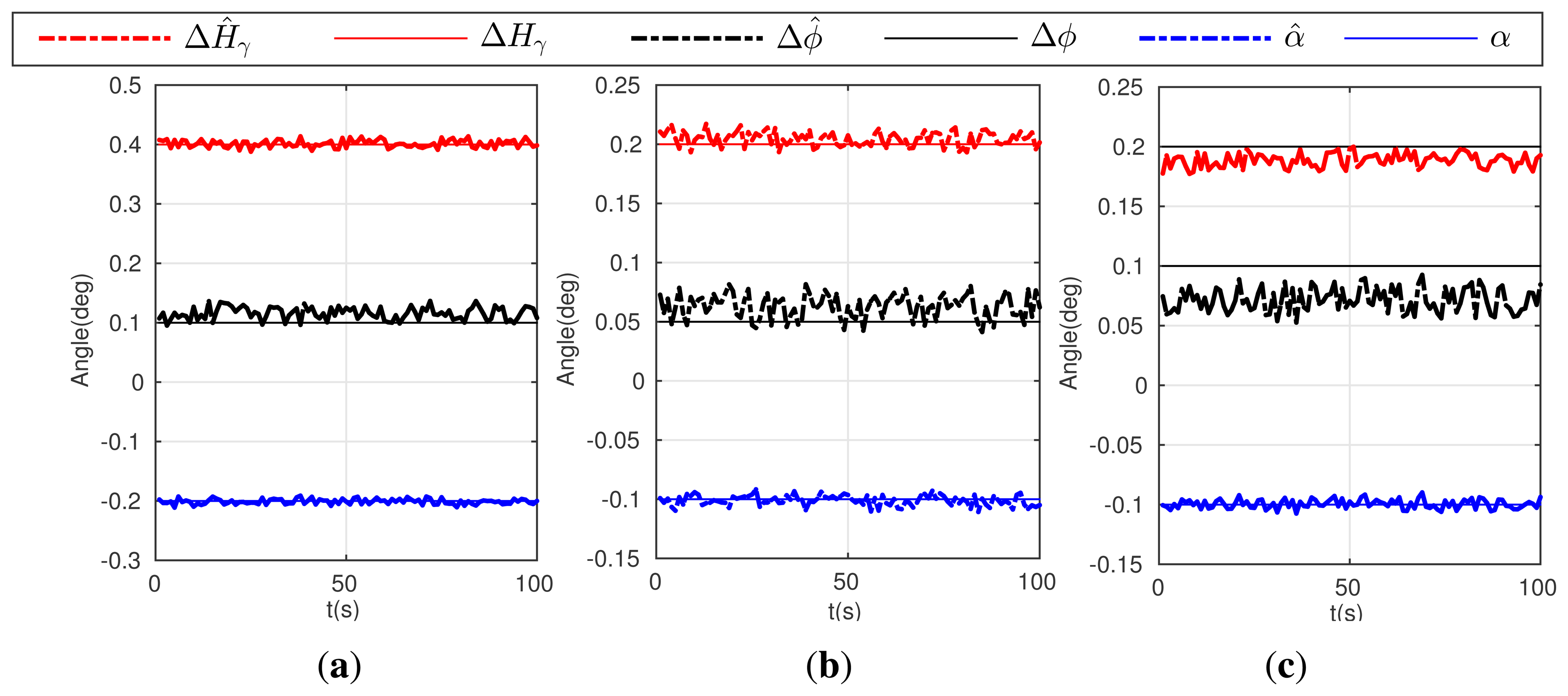
• Condition 5: α = γ = −0.2°, d_oR1 = 300 m, d_oR2 = 280 m, Δϕ = 0.1°, ΔH = 0.2°;

  where, d_oR1 denotes the distances between the point o and the reference point R₁, and d_oR2 for R₂.

• Condition 6: α = γ = −0.1°, d_oR1 = 300 m, d_oR2 = 280 m, Δϕ = 0.05°, ΔH = 0.1°;

• Condition 7: α = γ = −0.1°, d_oR1 = 200 m, d_oR2 = 140 m, Δϕ = 0.05°, ΔH = 0.1°;

  Figure 4 gives the simulation result of the first three conditions above (5,6,7).

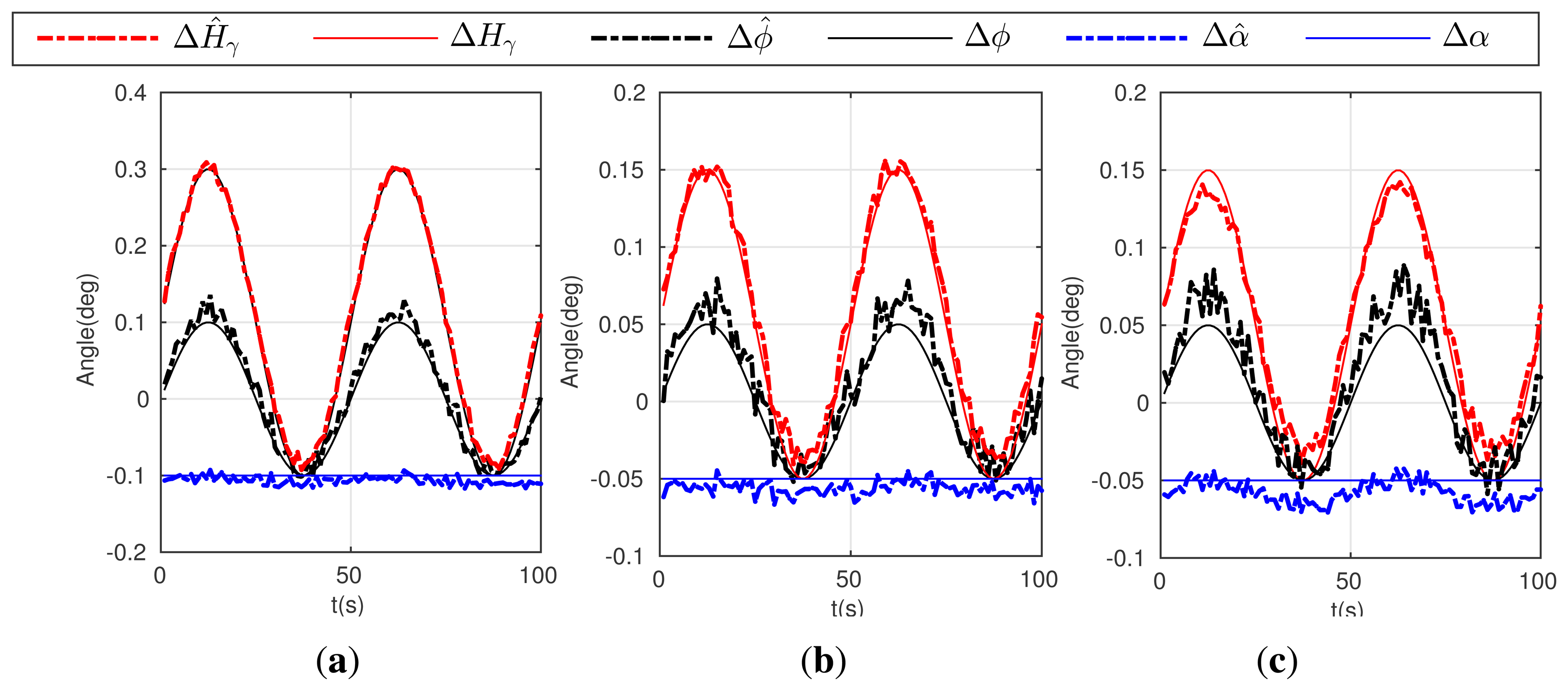
• Condition 8: α = γ = −0.2°, d_oR1 = 300 m, d_oR2 = 280 m, ΔH = 0.2° sin(2π × t/50), Δϕ = 0.1° sin(2π × t/50);

• Condition 9: α = γ = −0.1°, d_oR1 = 300 m, d_oR2 = 280 m, ΔH = 0.1° sin(2π × t/50), Δϕ = 0.05° sin(2π × t/50);

• Condition 10: α = γ = −0.1°, d_oR1 = 200 m, d_oR2 = 140 m, ΔH = 0.1° sin(2π × t/50), Δϕ = 0.05° sin(2π × t/50);

Figure 5 gives the simulation result of the later three conditions (8–10).

As shown in Figure 4a,b, although condition 5 and 6 give different error values, the calibration algorithm can realize accurate estimations. In comparing Figure 4b with 4c, the calibration accuracy decreases slightly, especially for the estimates of Δϕ̂ and ΔĤ_γ, when the reference points are much closer to observer. In addition, in the condition of varying errors, the proposed calibration algorithm can also estimate the types of errors given in condition 8, 9 and 10, which shows similar estimate performance seen in Figure 5a–c. Simulation results can prove that the calibration algorithm have a good performance in estimating both the installation and attitude measure error.

5.2. Simulation for Positioning Performance after Calibration

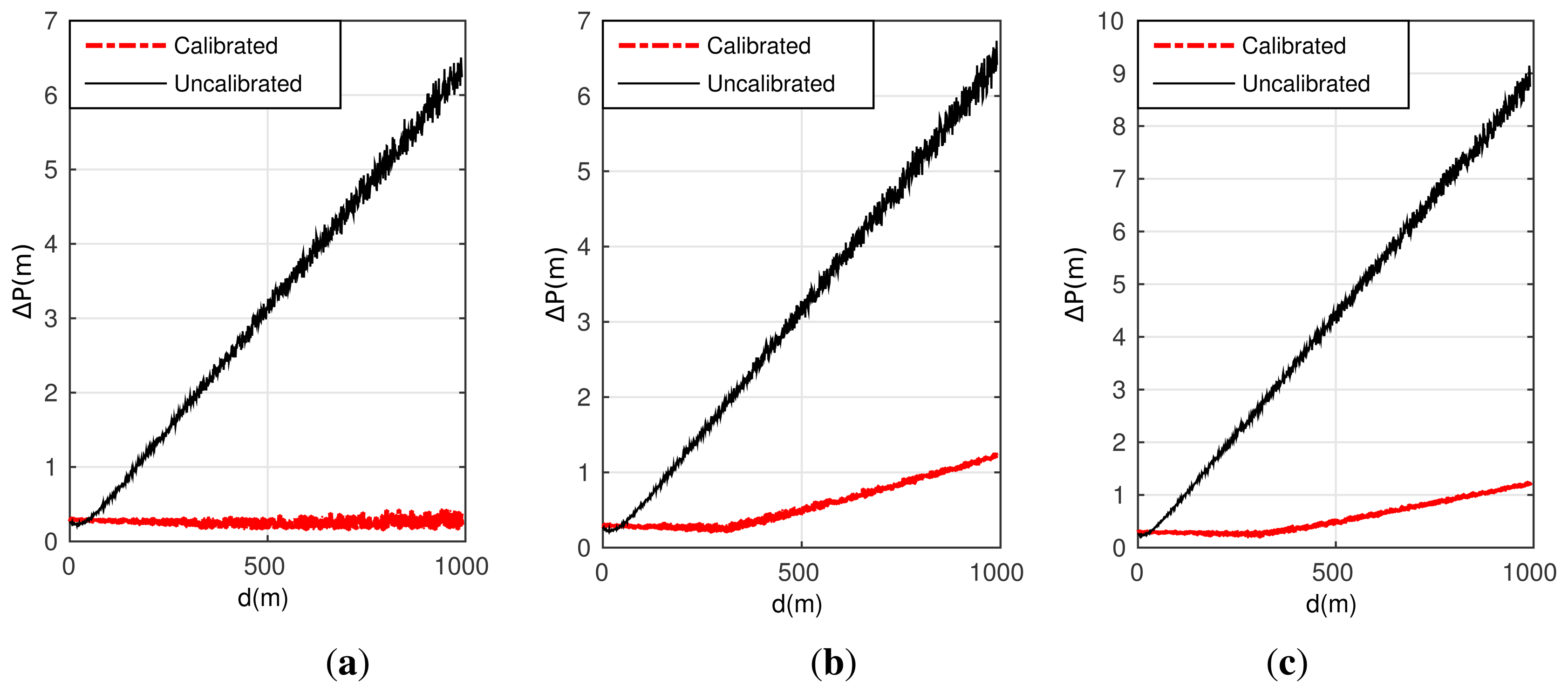
Simulations above demonstrates the calibration algorithm can realize simultaneous estimation of errors. Consequently, these estimated errors can be used for compensation, which would be very helpful for improving the positioning accuracy of target. Simulations under another three conditions are considered to evaluate the positioning performance of the scheme after simultaneously calibration.

• Condition 11: α = γ = −0.2°, d_oR1 = 300 m, d_oR2 = 280 m, Δϕ = 0.1°, ΔH = 0.2°; without considering the measurement error and noise of LDS;

• Condition 12: α = γ = −0.2°, d_oR1 = 300 m, d_oR2 = 280 m, Δϕ = 0.1°, ΔH = 0.2°;

• Condition 13: α = γ = −0.1°, d_oR1 = 200 m, d_oR2 = 140 m, Δϕ = 0.1°, ΔH = 0.2°;

Figure 6 gives the positioning performance comparison between the un-calibrated and calibrated approaches corresponding to these three conditions.

As shown in Figure 6, it is obvious that the position errors without calibration are much larger than the schemes adopt the designed calibration algorithm. When the measurement errors of LDS are not involved, the positioning error is close to zero at the distance of 1 km after well calibration, as seen in Figure 6a. Even when the measurement errors of LDS have been considered, the corresponding positioning errors in Figure 6b,c are accumulated but still less than 2 m at the distance of 1 km. As a result, the positioning approach based on INS/GPS/LDS and the simultaneously designed calibration algorithm gain an improvement on the positioning accuracy, and are extremely efficient for a long range of 1 km.

6. Conclusions

In this paper, we present a simultaneously calibration approach for an INS/GPS/LDS Target Tracker to compensate the installation and attitude Errors. This approach is based on the attitude and position measured by INS/GPS system, and the distance between observer and target measured by LDS. The installation error, which exists between INS/GPS and LDS subsystems, are focused and researched. Its influence on positioning performance is investigated. Then, a simultaneous calibration algorithm is designed to estimate both the installation error and the attitude error of INS/GPS. Finally, simulations are conducted to demonstrate the validity of the proposed calibration algorithm as well as the entire target positioning method.

As the following work, in the realization of the prototype, the low-cost Micro-electro-mechanical systems (MEMS) based INS could also be applied into this kind of system. In its corresponding calibration method, the property of MEMS/GPS/LDS should be analyzed. On the other hand, in the real test, the level-arm effect caused by introducing reference points should be considered.

References

- Blackman, S.S. Multiple-Target Tracking with Radar Applications; Artech House Inc.: Dedham, MA, USA, 1986; Volume 1, p. 463. [Google Scholar]
- Smith, D.; Singh, S. Approaches to multisensor data fusion in target tracking: A survey. IEEE Trans. Knowl. Data Eng. 2006, 18, 1696–1710. [Google Scholar]
- Luo, R.C.; Yih, C.C.; Su, K.L. Multisensor fusion and integration: Approaches, applications, and future research directions. IEEE Sens. J. 2002, 2, 107–119. [Google Scholar]
- Gui, C.; Mohapatra, P. Power conservation and quality of surveillance in target tracking sensor networks. Proceedings of the 10th Annual International Conference on Mobile Computing and Networking, Philadelphia, PA, USA, 26 September–1 October 2004; pp. 129–143.
- Benfold, B.; Reid, I. Stable multi-target tracking in real-time surveillance video. Proceedings of the 2011 IEEE Conference on Computer Vision and Pattern Recognition (CVPR), Providence, RI, USA, 20–25 June 2011; pp. 3457–3464.
- Nakabo, Y.; Ishikawa, M.; Toyoda, H.; Mizuno, S. 1 ms column parallel vision system and its application of high speed target tracking. Proceedings of the IEEE International Conference on Robotics and Automation, San Francisco, CA, USA, 24–28 April 2000; Volume 1, pp. 650–655.
- Zhou, K.; Roumeliotis, S.I. Multirobot active target tracking with combinations of relative observations. IEEE Trans. Robot. 2011, 27, 678–695. [Google Scholar]
- Li, X.R.; Jilkov, V.P. Survey of maneuvering target tracking. Part I. Dynamic models. IEEE Trans. Aerosp. Electron. Syst. 2003, 39, 1333–1364. [Google Scholar]
- Li, X.; Jilkov, V.P. Survey of maneuvering target tracking. Part II: Motion models of ballistic and space targets. IEEE Trans. Aerosp. Electron. Syst. 2010, 46, 96–119. [Google Scholar]
- Hue, C.; Le Cadre, J.P.; Pérez, P. Sequential Monte Carlo methods for multiple target tracking and data fusion. IEEE Trans. Signal Process. 2002, 50, 309–325. [Google Scholar]
- McGinnity, S.; Irwin, G.W. Multiple model bootstrap filter for maneuvering target tracking. IEEE Trans. Aerosp. Electron. Syst. 2000, 36, 1006–1012. [Google Scholar]
- Blackman, S.S. Multiple hypothesis tracking for multiple target tracking. IEEE Aerosp. Electron. Syst. Mag. 2004, 19, 5–18. [Google Scholar]
- Vermaak, J.; Godsill, S.J.; Perez, P. Monte carlo filtering for multi target tracking and data association. IEEE Aerosp. Electron. Syst. Mag. 2005, 41, 309–332. [Google Scholar]
- Bar-Shalom, Y. Multitarget-Multisensor Tracking: Advanced Applications; Artech House: Norwood, MA, USA, 1990; Volume 1, p. 391. [Google Scholar]
- Stone, L.D.; Streit, R.L.; Corwin, T.L.; Bell, K.L. Bayesian Multiple Target Tracking; Artech House: Boston, MA, USA, 2013. [Google Scholar]
- Bole, A.G.; Dineley, W.O.; Wall, A.D. Radar and ARPA Manual: Radar, AIS and Target Tracking for Marine Radar Users; Butterworth-Heinemann: Oxford, UK, 2013. [Google Scholar]
- Mao, Y.; Zhou, X.; Zhang, J. Passive radar tracking of a maneuvering target using variable structure multiple-model algorithm. Proceedings of the Fifth International Conference on Machine Vision (ICMV 2012), Wuhan, China, 20–21 October 2012.
- Howland, P.E. Target tracking using television-based bistatic radar. IEEE Proc. Radar Sonar Navig. 1999, 146, 166–174. [Google Scholar]
- Gordon, N. A hybrid bootstrap filter for target tracking in clutter. IEEE Trans. Aerosp. Electron. Syst. 1997, 33, 353–358. [Google Scholar]
- Arnold, J.; Shaw, S.; Pasternack, H. Efficient target tracking using dynamic programming. IEEE Trans. Aerosp. Electron. Syst. 1993, 29, 44–56. [Google Scholar]
- Li, T.; Chang, S.J.; Tong, W. Fuzzy target tracking control of autonomous mobile robots by using infrared sensors. IEEE Trans. Fuzzy Syst. 2004, 12, 491–501. [Google Scholar]
- Yilmaz, A.; Shafique, K.; Shah, M. Target tracking in airborne forward looking infrared imagery. Image Vis. Comput. 2003, 21, 623–635. [Google Scholar]
- Pellegrini, S.; Ess, A.; Schindler, K.; Van Gool, L. You’ll never walk alone: Modeling social behavior for multi-target tracking. Proceedings of the 2009 IEEE 12th International Conference on Computer Vision, Kyoto, Japan, 29 September–2 October 2009; pp. 261–268.
- Benavidez, P.; Jamshidi, M. Mobile robot navigation and target tracking system. Proceedings of the 2011 6th International Conference on System of Systems Engineering, Albuquerque, NM, USA, 27–30 June 2011; pp. 299–304.
- Choi, W.; Savarese, S. Multiple target tracking in world coordinate with single, minimally calibrated camera. Proceedings of the 11th European Conference on Computer Vision, Crete, Greece, 5–11 September 2010; pp. 553–567.
- Granstrom, K.; Lundquist, C.; Orguner, O. Extended target tracking using a Gaussian-mixture PHD filter. IEEE Trans. Aerosp. Electron. Syst. 2012, 48, 3268–3286. [Google Scholar]
- Kilambi, S.; Tipton, S. Development of an algorithm to measure defect geometry using a 3D laser scanner. Measur. Sci. Technol. 2012, 23. [Google Scholar] [CrossRef]
- Chen, W.P.; Hou, J.C.; Sha, L. Dynamic clustering for acoustic target tracking in wireless sensor networks. IEEE Trans. Mob. Comput. 2004, 3, 258–271. [Google Scholar]
- Liu, J.; Reich, J.; Zhao, F. Collaborative in-network processing for target tracking. EURASIP J. Appl. Signal Process. 2003, 2003, 378–391. [Google Scholar]
- Atia, G.K.; Veeravalli, V.V.; Fuemmeler, J.A. Sensor scheduling for energy-efficient target tracking in sensor networks. IEEE Trans. Signal Process. 2011, 59, 4923–4937. [Google Scholar]
- Mourad, F.; Chehade, H.; Snoussi, H.; Yalaoui, F.; Amodeo, L.; Richard, C. Controlled mobility sensor networks for target tracking using ant colony optimization. IEEE Trans. Mob. Comput. 2012, 11, 1261–1273. [Google Scholar]
- Kim, W.; Mechitov, K.; Choi, J.Y.; Ham, S. On target tracking with binary proximity sensors. Proceedings of the International Symposium on Information Processing in Sensor Networks, Los Angeles, CA, USA, 15 April 2005; pp. 301–308.
- Song, L.; Wang, Y. Multiple target counting and tracking using binary proximity sensors: Bounds, coloring, and filter. Proceedings of the 15th ACM International Symposium on Mobile Ad Hoc Networking and Computing, Philadelphia, PA, USA, 11–14 August 2014; pp. 397–406.
- Guohui, Z. Measurement of topography deformation based on 3D laser scanner. Chin. J. Sci. Instrum. 2006, 27, 96–97. [Google Scholar]
- Cheng, J.; Landry, R.; Chen, D.; Guan, D. A Novel Method for Target Navigation and Mapping Based on Laser Ranging and MEMS/GPS Navigation. J. Appl. Math. 2014, 2014. [Google Scholar] [CrossRef]
- Aydemir, G.A.; Saranlı, A. Characterization and calibration of MEMS inertial sensors for state and parameter estimation applications. Measurement 2012, 45, 1210–1225. [Google Scholar]
- Stebler, Y.; Guerrier, S.; Skaloud, J.; Victoria-Feser, M. A framework for inertial sensor calibration using complex stochastic error models. Proceedings of the Position Location and Navigation Symposium (PLANS), Myrtle Beach, SC, USA, 23–26 April 2012; pp. 849–861.
- Chen, C.; Liu, H.; Liu, Y.; Zhuo, X. High accuracy calibration for vehicle-based laser scanning and urban panoramic imaging and surveying system. Proc. SPIE 2013, 8917. [Google Scholar] [CrossRef]
- Kocmanova, P.; Zalud, L.; Chromy, A. 3D proximity laser scanner calibration. Proceedings of the 2013 18th International Conference on Methods and Models in Automation and Robotics (MMAR), Miedzyzdroje, Poland, 26–29 August 2013; pp. 742–747.
- Niu, X.; Nassar, S.; El-Sheimy, N. An accurate land-vehicle MEMS IMU/GPS navigation system using 3D auxiliary velocity updates. Navigation 2007, 54, 177–188. [Google Scholar]
- Acuity. AccuRange AR500 Laser Sensor User’s Manual. Available online: http://www.disensors.com/downloads/products/AR500 (accessed on 20 October 2014).
- Leica. DISTO D810 Touch. Available online: http://www.leica-geosystems.com/en/Leica-DISTO-D810-touch_104560.htm (accessed on 20 October 2014).
- Bosch. GLM-80 Laser Distance and Angle Measurer. Available online: http://www.boschtools.com/Products/Tools/Pages/BoschProductDetail.aspx?pid=GLM (accessed on 20 October 2014).
- Hilti. PD-I Laser Range Meter. Available online: https://www.us.hilti.com/measuring-systems/laser-range-meters/r587754 (accessed on 20 October 2014).
- Fu, Q.W.; Qin, Y.Y.; Zhang, J.H.; Li, S.H. Rapid recursive least-square fine alignment method for SINS. Zhongguo Guanxing Jishu Xuebao 2012, 20. [Google Scholar] [CrossRef]
© 2015 by the authors; licensee MDPI, Basel, Switzerland. This article is an open access article distributed under the terms and conditions of the Creative Commons Attribution license ( http://creativecommons.org/licenses/by/4.0/).
Share and Cite
Cheng, J.; Chen, D.; Sun, X.; Wang, T. A Simultaneously Calibration Approach for Installation and Attitude Errors of an INS/GPS/LDS Target Tracker. Sensors 2015, 15, 3575-3592. https://doi.org/10.3390/s150203575
Cheng J, Chen D, Sun X, Wang T. A Simultaneously Calibration Approach for Installation and Attitude Errors of an INS/GPS/LDS Target Tracker. Sensors. 2015; 15(2):3575-3592. https://doi.org/10.3390/s150203575
Chicago/Turabian StyleCheng, Jianhua, Daidai Chen, Xiangyu Sun, and Tongda Wang. 2015. "A Simultaneously Calibration Approach for Installation and Attitude Errors of an INS/GPS/LDS Target Tracker" Sensors 15, no. 2: 3575-3592. https://doi.org/10.3390/s150203575