
The Bubble Box: Towards an Automated Visual Sensor for 3D Analysis and Characterization of Marine Gas Release Sites

Abstract
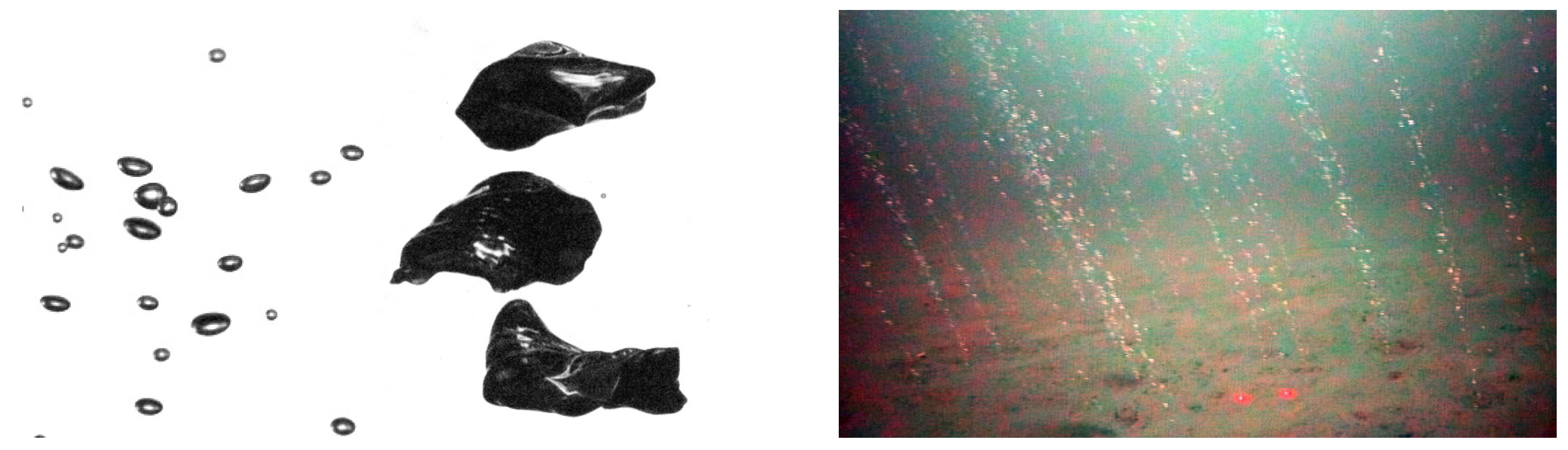
:1. Introduction


State of the Art in Visual Characterization of Bubble Streams
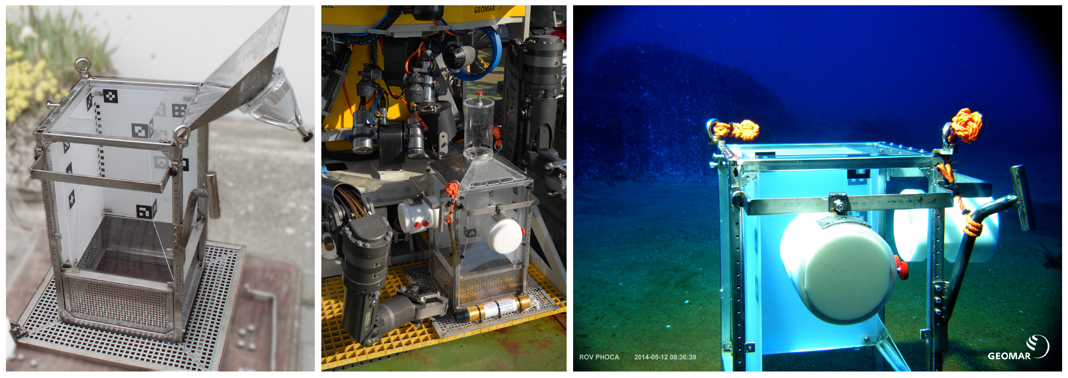
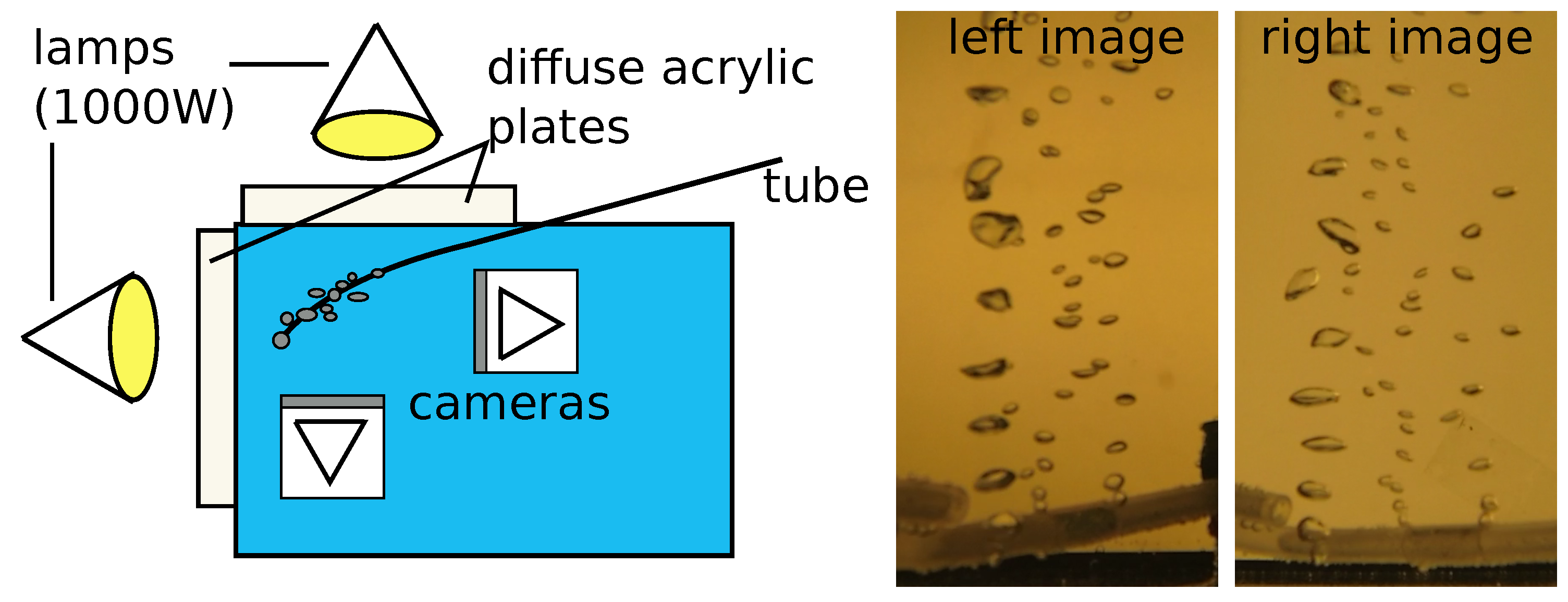
2. Bubble Box Design and Calibration
2.1. Design Considerations
2.2. Calibration
2.2.1. Synchronization
2.2.2. Stereo Calibration
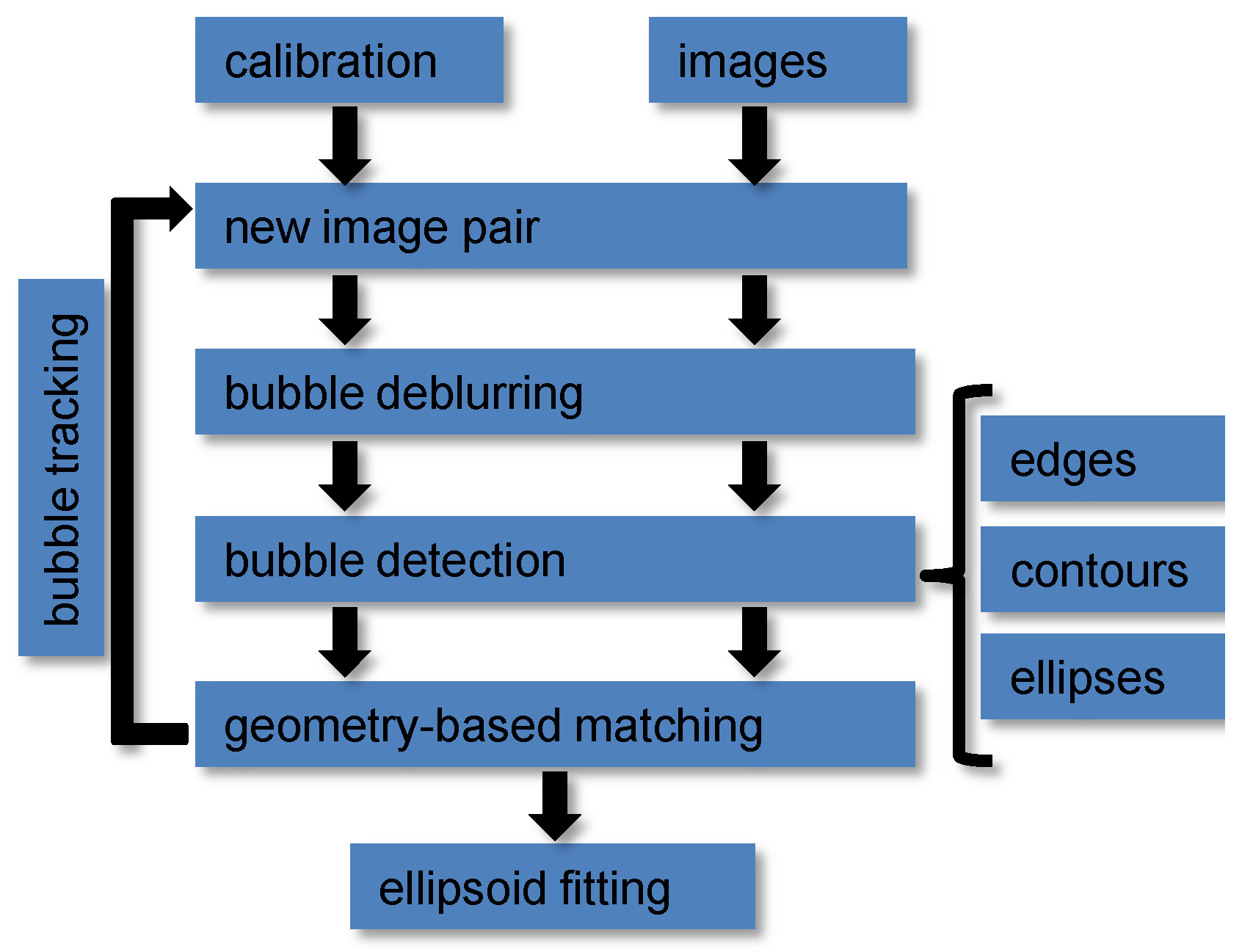
3. Bubble Stream Characterization

3.1. Preprocessing—Automatic Region of Interest Selection
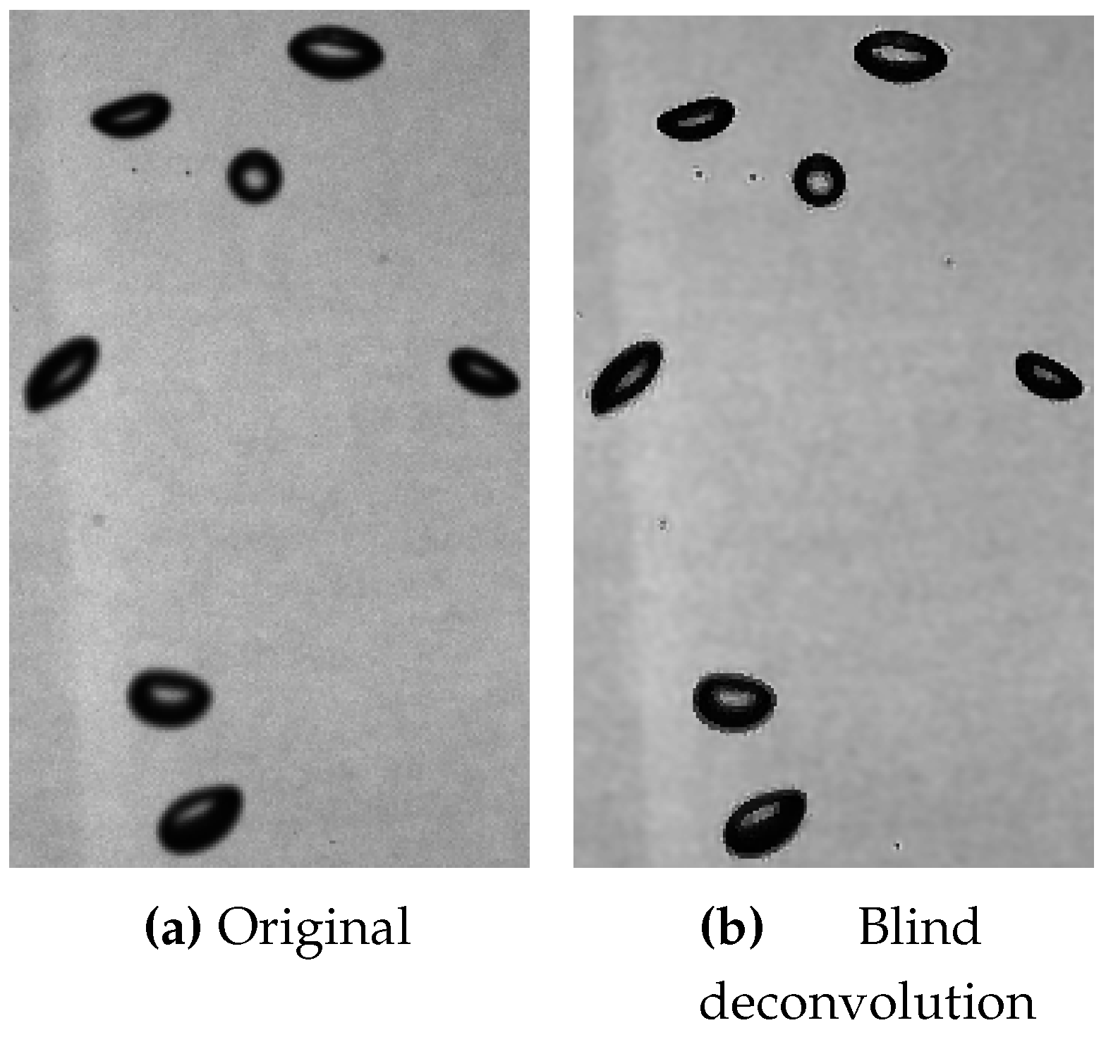
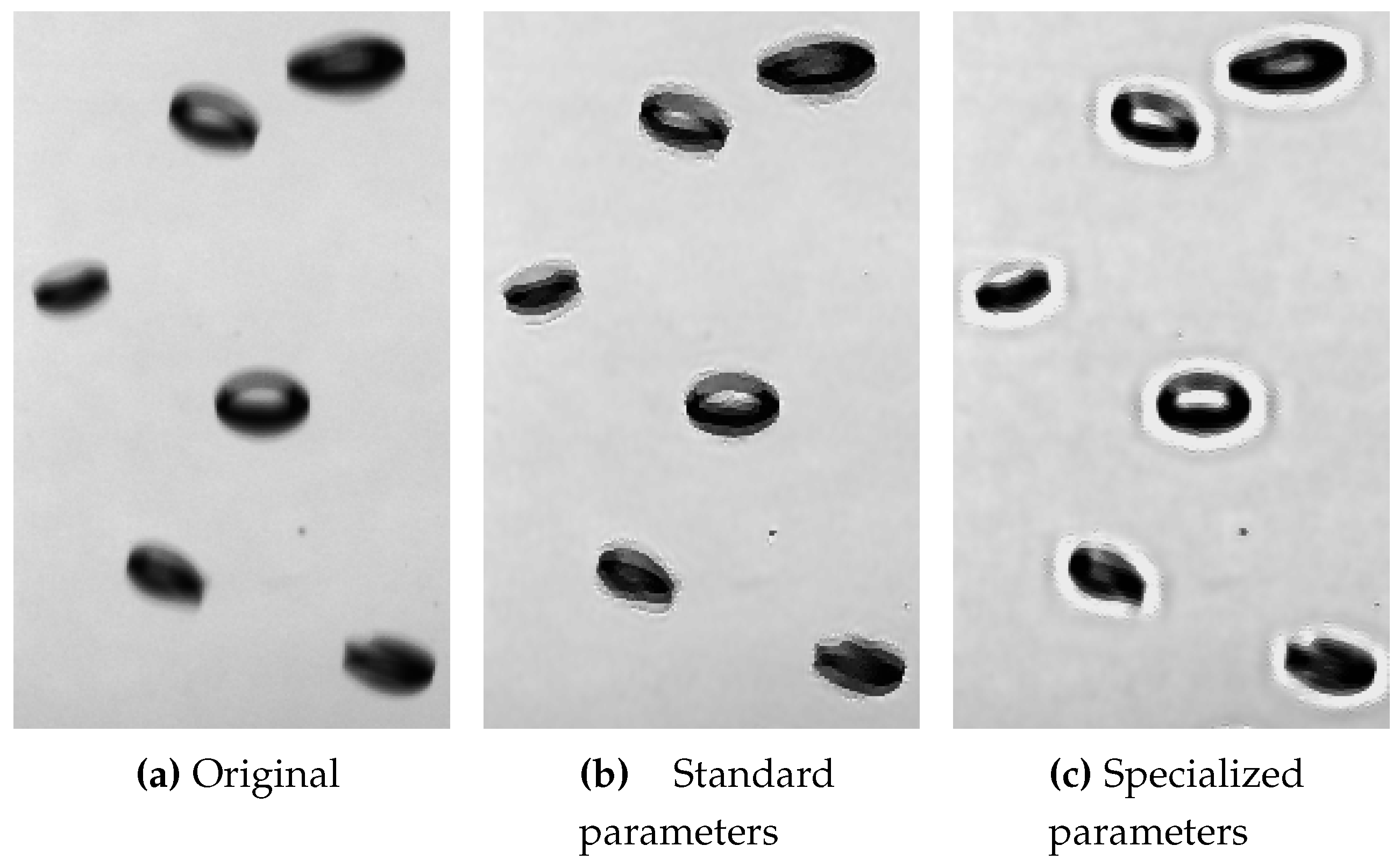
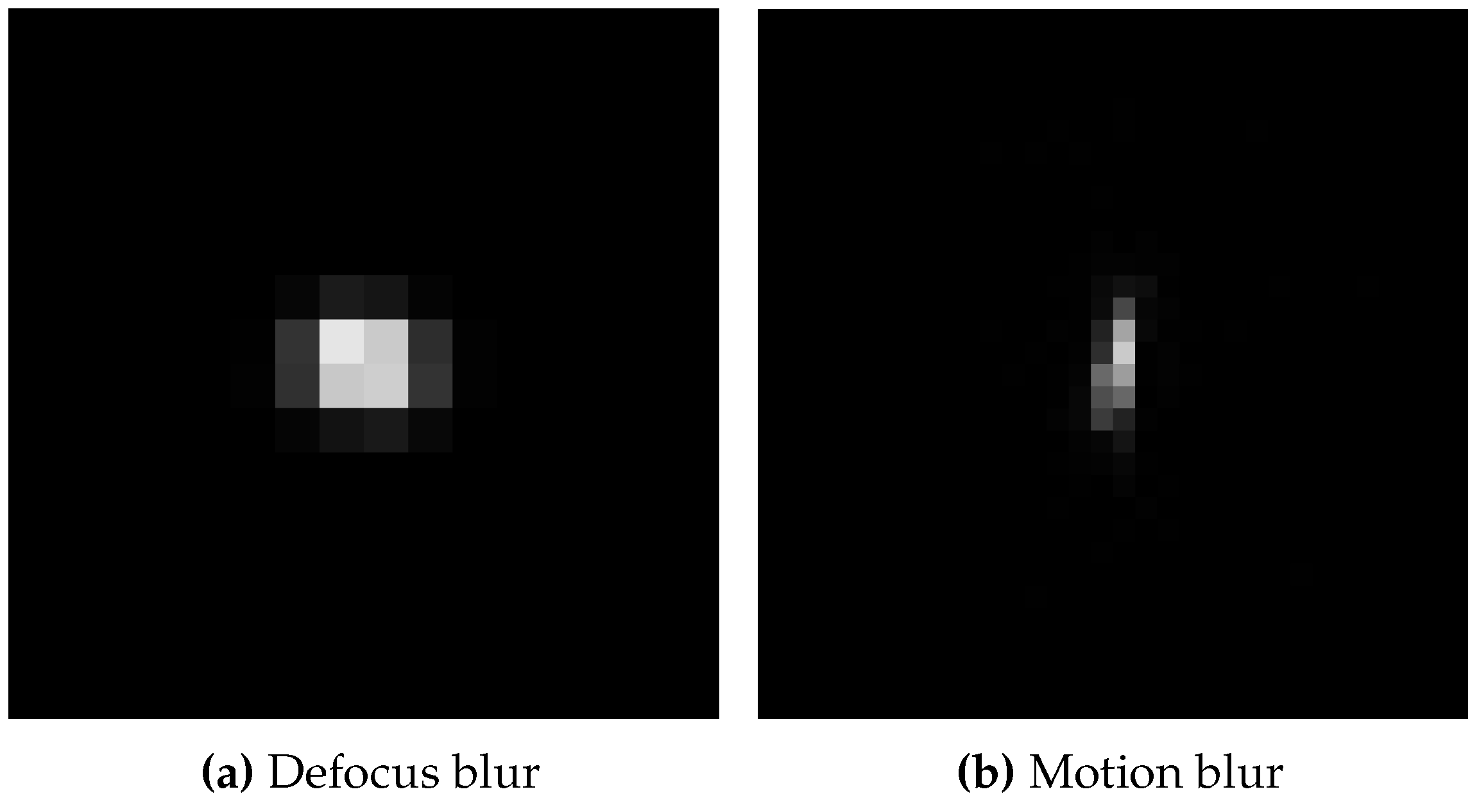
3.2. Preprocessing—Bubble Deblurring
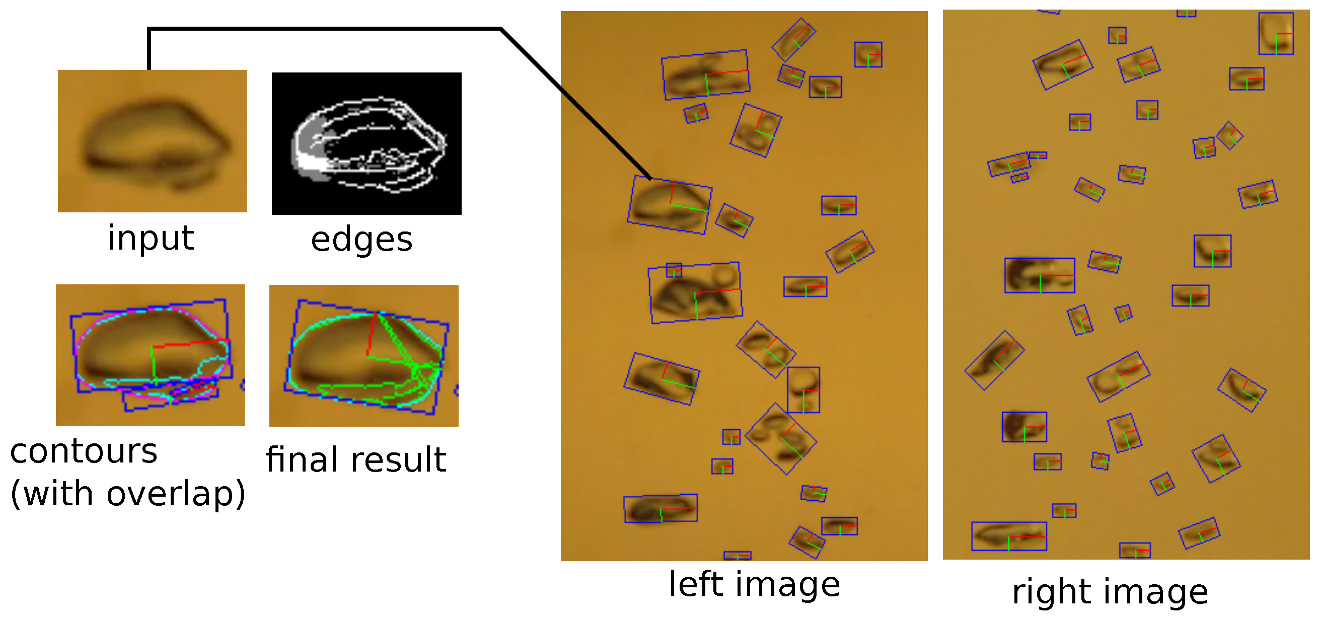
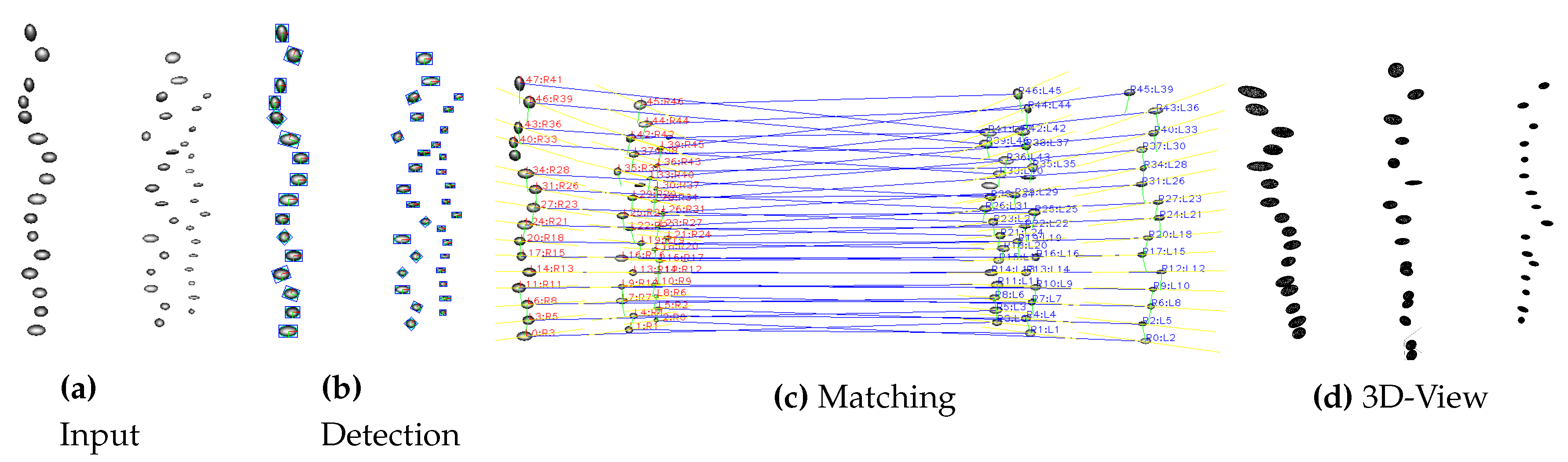
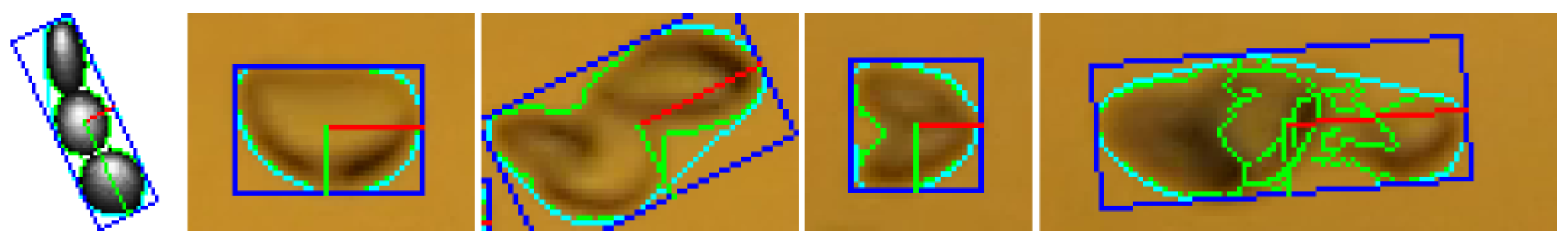
3.3. Bubble Detection

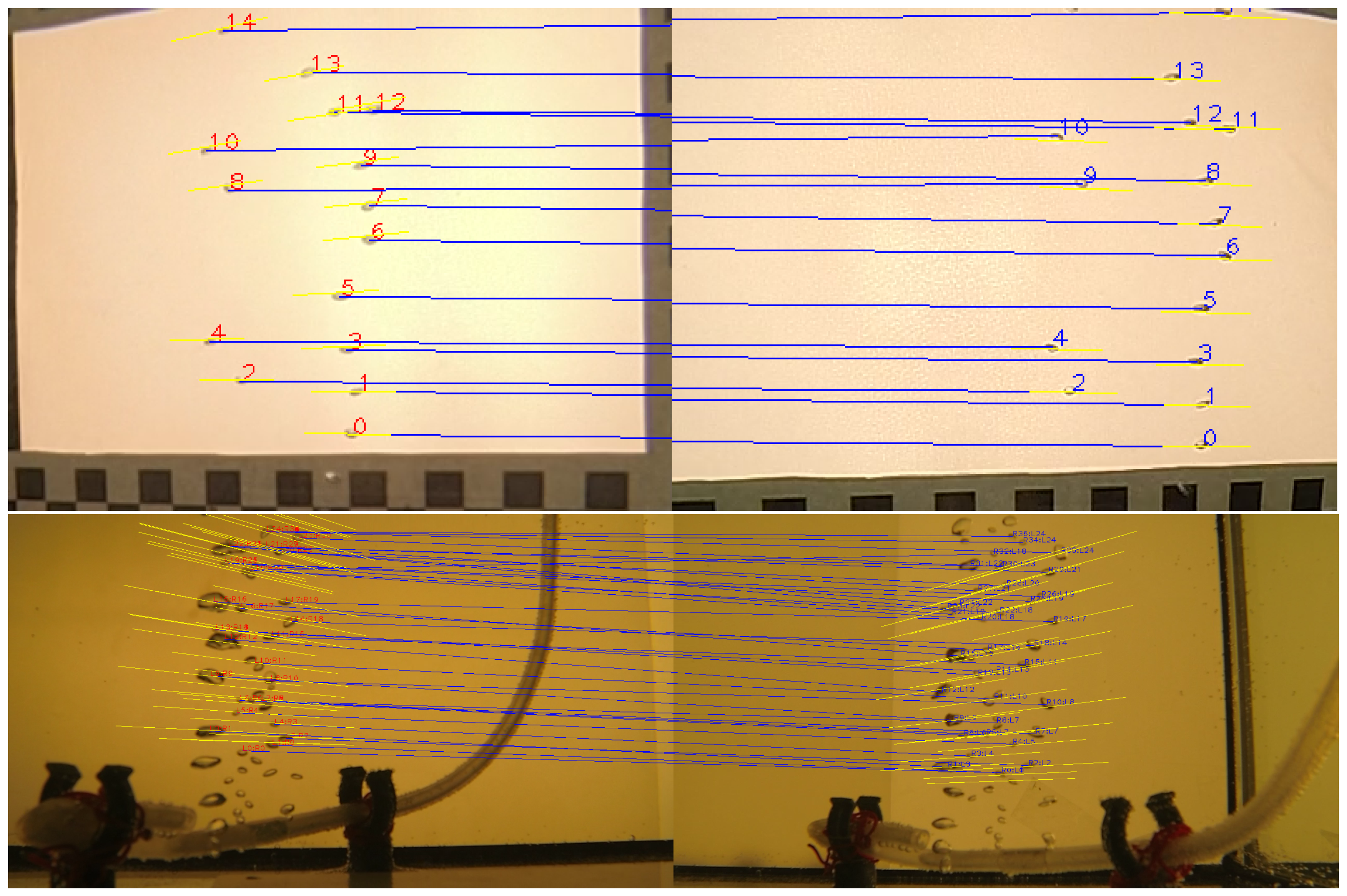
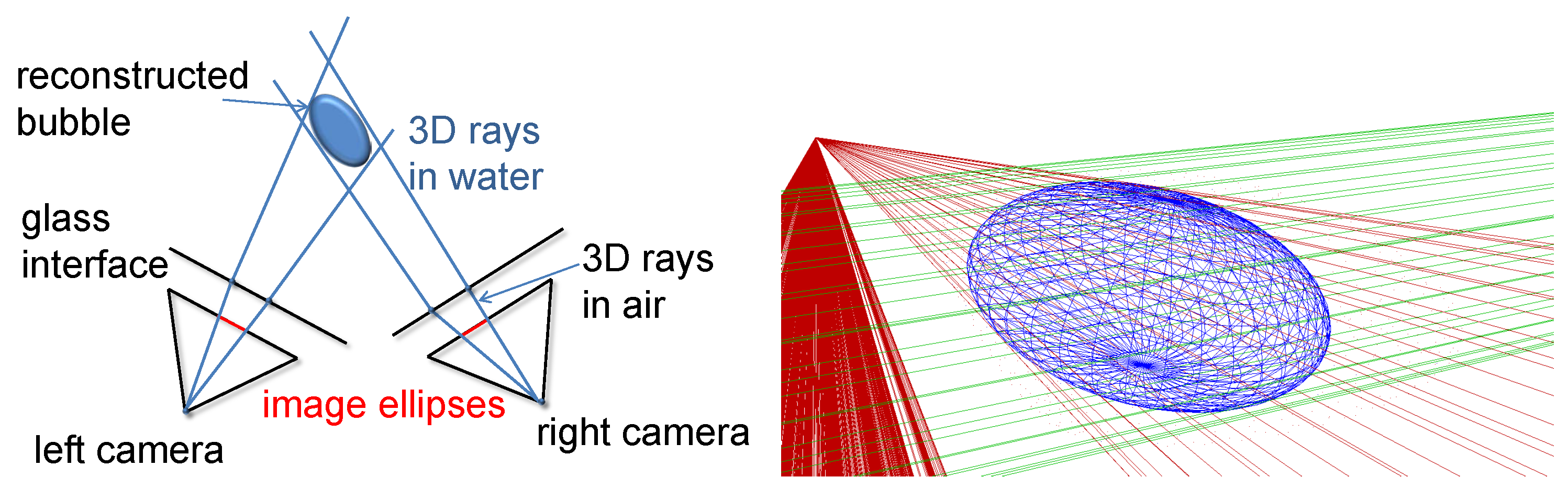
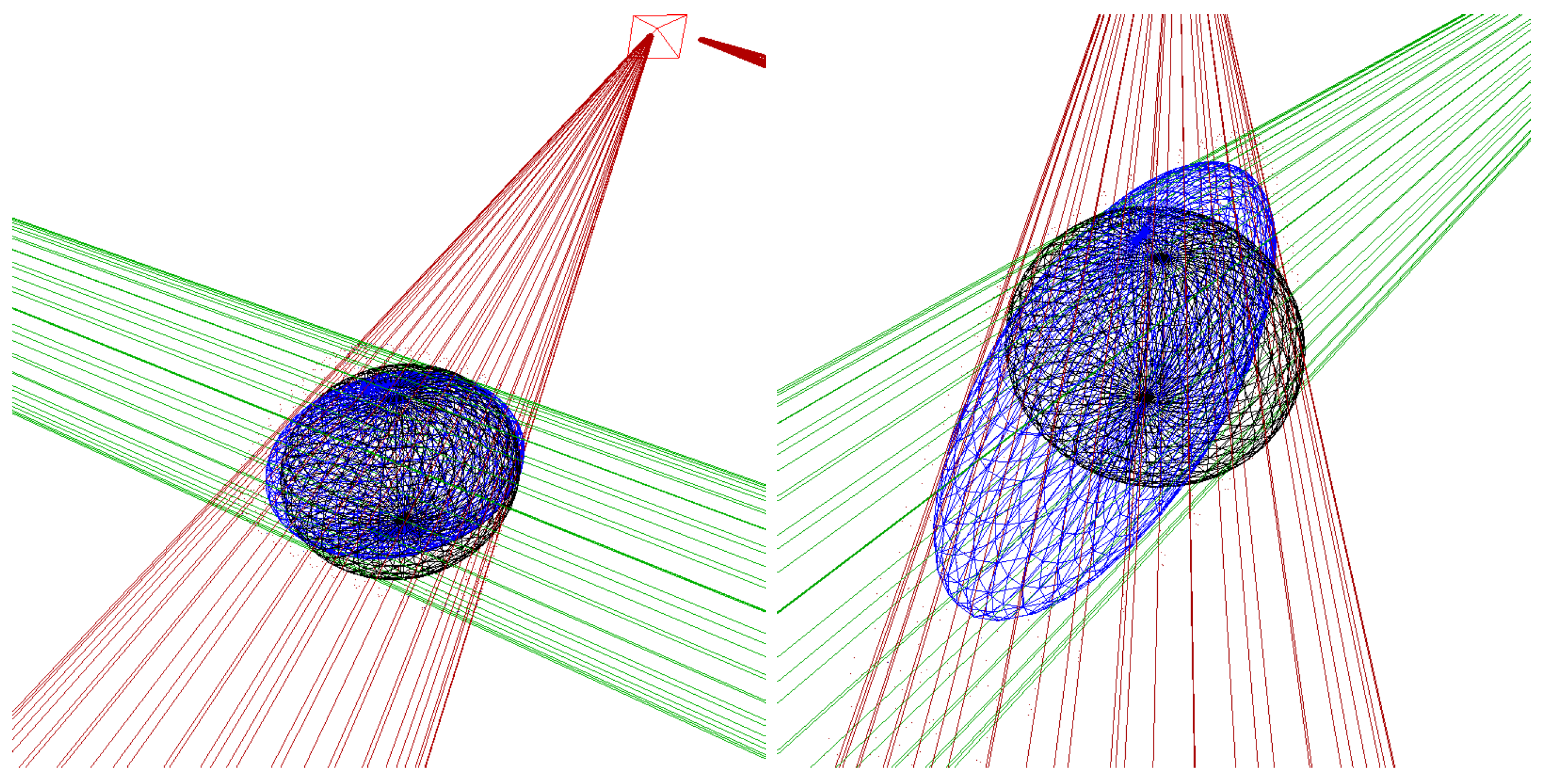
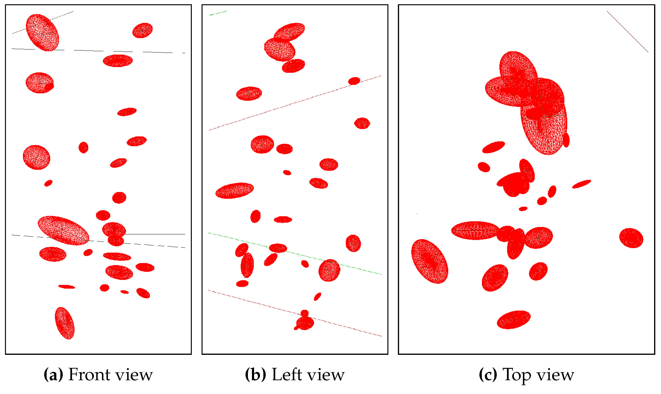
3.4. Stereo Matching and Ellipsoid Triangulation


3.5. Bubble Tracking
4. Assessment
4.1. Deblurring


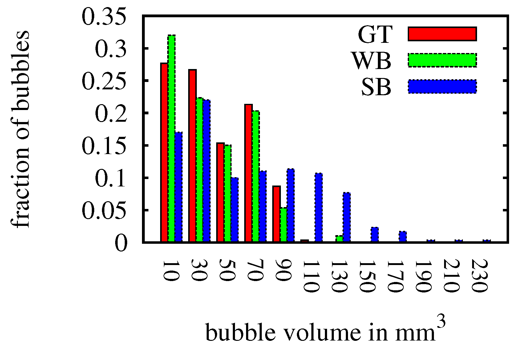
4.2. Bubble Simulator


| Ground Truth | WB | SB | Mono | |
|---|---|---|---|---|
| Synthetic Data | ||||
| volume | 127,85.72 mm | 11,391.93 mm | 18,823.21 mm | 15,028.2 mm |
| average volume | 42.62 mm | 39.83 mm | 66.04 mm | 52.18 mm |
| average velocity | 35.94 cm·s | 36.00 cm·s | 36.16 cm·s | - |
| # bubbles | 300 | 286 | 285 | 288 |


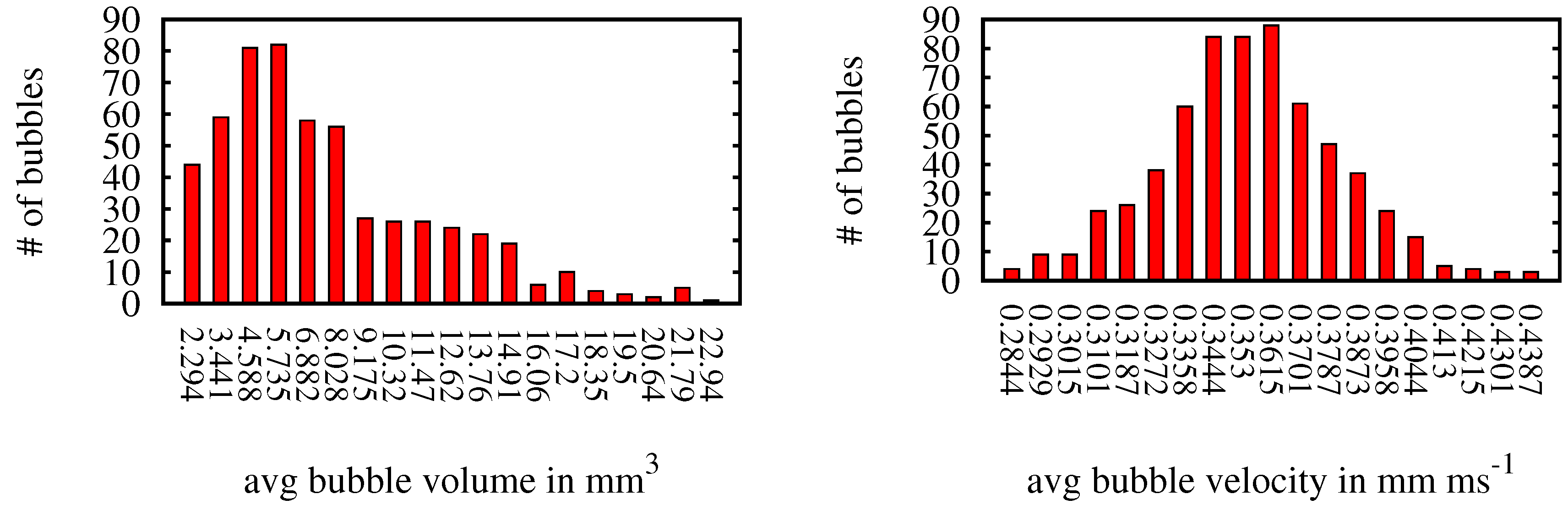
4.3. Test Setup with Air Bubbles in Water
| Measured | Results | Comment | |
|---|---|---|---|
| Real Data | |||
| flux | 4.177 mL·s | 2.504 mL·s | estimated volume of missed bubbles 0.291–0.7488 mL·s |
| velocity | - | 36.135 cm·s | - |
5. Discussion
6. Conclusion
Acknowledgments
Author Contributions
Conflicts of Interest
References
- Fleischer, P.; Orsi, T.; Richardson, M.; Anderson, A. Distribution of free gas in marine sediments: A global overview. Geo-Mar. Lett. 2001, 21, 103–122. [Google Scholar]
- Judd, A. Natural seabed gas seeps as sources of atmospheric methane. Environ. Geol. 2004, 46, 988–996. [Google Scholar]
- Clift, R.; Grace, J.R.; Weber, M.E. Bubbles, Drops, and Particles; Academic Press: Waltham, MA, USA, 1978. [Google Scholar]
- Ciais, P.; Sabine, C.; Bala, G.; Bopp, L.; Brovkin, V.; Canadell, J.; Chhabra, A.; DeFries, R.; Galloway, J.; Heimann, M.; et al. Carbon and Other Biogeochemical Cycles. In Climate Change 2013: The Physical Science Basis. Contribution of Working Group I to the Fifth Assessment Report of the Intergovernmental Panel on Climate Change; Cambridge University Press: New York, NY, USA, 2013. [Google Scholar]
- Sommer, S.; Pfannkuche, O.; Linke, P.; Luff, R.; Greinert, J.; Drews, M.; Gubsch, S.; Pieper, M.; Poser, M.; Viergutz, T. Efficiency of the benthic filter: Biological control of the emission of dissolved methane from sediments containing shallow gas hydrates at Hydrate Ridge. Glob. Biogeochem. Cycles 2006, 20, 650–664. [Google Scholar]
- Chadwick, W.W.; Merle, S.G.; Buck, N.J.; Lavelle, J.W.; Resing, J.A.; Ferrini, V. Imaging of CO2 bubble plumes above an erupting submarine volcano, NW Rota-1, Mariana Arc. Geochem. Geophys. Geosyst. 2014, 15, 4325–4342. [Google Scholar] [CrossRef]
- Vielstädte, L.; Karstens, J.; Haeckel, M.; Schmidt, M.; Linke, P.; Reimann, S.; Liebetrau, V.; McGinnis, D.F.; Wallmann, K. Quantification of methane emissions at abandoned gas wells in the Central North Sea. Mar. Pet. Geol. 2015, in press. [Google Scholar] [CrossRef]
- Schneider von Deimling, J.; Linke, P.; Schmidt, M.; Rehder, G. Ongoing methane discharge at well site 22/4b (North Sea) and discovery of a spiral vortex bubble plume motion. Mar. Pet. Geol. 2015. [Google Scholar]
- Leifer, I.; Patro, R.K. The bubble mechanism for methane transport from the shallow sea bed to the surface: A review and sensitivity study. Cont. Shelf Res. 2002, 22, 2409–2428. [Google Scholar] [CrossRef]
- McGinnis, D.F.; Greinert, J.; Artemov, Y.; Beaubien, S.E.; Wüest, A. Fate of rising methane bubbles in stratified waters: How much methane reaches the atmosphere? J. Geophys. Res. Oceans 2006, 111, 141–152. [Google Scholar] [CrossRef]
- Leifer, I.; Boles, J. Measurement of marine hydrocarbon seep flow through fractured rock and unconsolidated sediment. Mar. Pet. Geol. 2005, 22, 551–568. [Google Scholar] [CrossRef]
- Leifer, I.; Culling, D. Formation of seep bubble plumes in the Coal Oil Point seep field. Geo-Mar. Lett. 2010, 30, 339–353. [Google Scholar] [CrossRef]
- Rehder, G.; Brewer, P.W.; Peltzer, E.T.; Friederich, G. Enhanced lifetime of methane bubble streams within the deep ocean. Geophys. Res. Lett. 2002, 29, 21-1–21-4. [Google Scholar] [CrossRef]
- Merewether, R.; Olsson, M.S.; Lonsdale, P. Acoustically detected hydrocarbon plumes rising from 2-km depths in Guaymas Basin, Gulf of California. J. Geophys. Res. Solid Earth 1985, 90, 3075–3085. [Google Scholar] [CrossRef]
- Greinert, J. Monitoring temporal variability of bubble release at seeps: The hydroacoustic swath system GasQuant. J. Geophys. Res. Oceans 2008, 113, 827–830. [Google Scholar] [CrossRef]
- Schneider von Deimling, J.; Brockhoff, J.; Greinert, J. Flare imaging with multibeam systems: Data processing for bubble detection at seeps. Geochem. Geophys. Geosyst. 2007, 8, 57–77. [Google Scholar]
- Colbo, K.; Ross, T.; Brown, C.; Weber, T. A review of oceanographic applications of water column data from multibeam echosounders. Estuar. Coast. Shelf Sci. 2014, 145, 41–56. [Google Scholar] [CrossRef]
- Schneider von Deimling, J.; Papenberg, C. Technical Note: Detection of gas bubble leakage via correlation of water column multibeam images. Ocean Sci. 2012, 8, 175–181. [Google Scholar] [Green Version]
- Veloso, M.; Greinert, J.; Mienert, J.; de Batist, M. A new methodology for quantifying bubble flow rates in deep water using splitbeam echosounders: Examples from the Arctic offshore NW-Svalbard. Limnol. Oceanogr. Methods 2015, 13, 267–287. [Google Scholar] [CrossRef]
- Leifer, I.; de Leeuw, G.; Cohen, L.H. Optical Measurement of Bubbles: System Design and Application. J. Atmos. Ocean. Technol. 2003, 20, 1317–1332. [Google Scholar] [CrossRef]
- Thomanek, K.; Zielinski, O.; Sahling, H.; Bohrmann, G. Automated gas bubble imaging at sea floor—A new method of in situ gas flux quantification. Ocean Sci. 2010, 6, 549–562. [Google Scholar]
- Wang, B.; Socolofsky, S.A. A deep-sea, high-speed, stereoscopic imaging system for in situ measurement of natural seep bubble and droplet characteristics. Deep Sea Res. I Oceanogr. Res. Pap. 2015, 104, 134–148. [Google Scholar] [CrossRef]
- Leifer, I. Characteristics and scaling of bubble plumes from marine hydrocarbon seepage in the Coal Oil Point seep field. J. Geophys. Res. Oceans 2010, 115, 45–54. [Google Scholar] [CrossRef]
- Sahling, H.; Bohrmann, G.; Artemov, Y.G.; Bahr, A.; Brüning, M.; Klapp, S.A.; Klaucke, I.; Kozlova, E.; Nikolovska, A.; Pape, T.; et al. Vodyanitskii mud volcano, Sorokin trough, Black Sea: Geological characterization and quantification of gas bubble streams. Mar. Pet. Geol. 2009, 26, 1799–1811. [Google Scholar] [CrossRef]
- Xue, T.; Qu, L.; Wu, B. Matching and 3-D Reconstruction of Multibubbles Based on Virtual Stereo Vision. IEEE Trans. Instrum. Measur. 2014, 63, 1639–1647. [Google Scholar]
- Bian, Y.; Dong, F.; Zhang, W.; Wang, H.; Tan, C.; Zhang, Z. 3D reconstruction of single rising bubble in water using digital image processing and characteristic matrix. Particuology 2013, 11, 170–183. [Google Scholar] [CrossRef]
- Kotowski, R. Phototriangulation in multi-media photogrammetry. Int. Arch. Photogramm. Remote Sens. 1988, 27, B5. [Google Scholar]
- Jordt-Sedlazeck, A.; Koch, R. Refractive Calibration of Underwater Cameras. In Computer Vision–ECCV 2012; Fitzgibbon, A., Lazebnik, S., Perona, P., Sato, Y., Schmid, C., Eds.; Springer: Berlin, Germany, 2012; Volume 7576, pp. 846–859. [Google Scholar]
- Jordt, A. Underwater 3D Reconstruction Based on Physical Models for Refraction and Underwater Light Propagation. Ph.D. Thesis, Kiel University, Kiel, Germany, 2013. [Google Scholar]
- Zelenka, C. Gas Bubble Shape Measurement and Analysis. In Pattern Recognition, Proceedings of the 36th German Conference on Pattern Recognition, (GCPR 2014), Münster, Germany, 2–5 September 2014; pp. 743–749.
- Brown, D.C. Close-range camera calibration. Photogramm. Eng. 1971, 37, 855–866. [Google Scholar]
- Schiller, I.; Beder, C.; Koch, R. Calibration of a PMD-camera using a planar calibration pattern together with a multi-camera setup. Int. Arch. Photogramm. Remote Sens. Spat. Inf. Sci. 2008, 21, 297–302. [Google Scholar]
- Treibitz, T.; Schechner, Y.Y.; Kunz, C.; Singh, H. Flat Refractive Geometry. IEEE Trans. Pattern Anal. Mach. Intell. 2012, 34, 51–65. [Google Scholar] [CrossRef] [PubMed]
- Agrawal, A.; Ramalingam, S.; Taguchi, Y.; Chari, V. A theory of multi-layer flat refractive geometry. In Proceedings of the IEEE Conference on Computer Vision and Pattern Recognition (CVPR), Providence, RI, USA, 16–21 June 2012; pp. 3346–3353.
- Harvey, E.S.; Shortis, M.R. Calibration stability of an underwater stereo-video system: Implications for measurement accuracy and precision. Mar. Technol. Soc. J. 1998, 32, 3–17. [Google Scholar]
- Farnebäck, G. Two-frame Motion Estimation Based on Polynomial Expansion. In Image Analysis, Proceedings of the 13th Scandinavian Conference, Halmstad, Sweden, 29 June–2 July 2003; Springer-Verlag: Berlin, Germany, 2003; pp. 363–370. [Google Scholar]
- Born, M.; Wolf, E. Principles of Optics: Electromagnetic Theory of Propagation, Interference and Diffraction of Light, 6th ed.; Pergamon Press: Oxford, UK; New York, NY, USA, 1980. [Google Scholar]
- Zelenka, C.; Koch, R. Blind Deconvolution on Underwater Images for Gas Bubble Measurement. Int. Arch. Photogramm. Remote Sens. Spa. Inf. Sci. 2015, XL-5/W5, 239–244. [Google Scholar] [CrossRef]
- Levin, A.; Weiss, Y.; Durand, F.; Freeman, W.T. Understanding Blind Deconvolution Algorithms. IEEE Trans. Pattern Anal. Mach. Intell. 2011, 33, 2354–2367. [Google Scholar] [CrossRef] [PubMed]
- Perrone, D.; Favaro, P. Total Variation Blind Deconvolution: The Devil Is in the Details. In Proceedings of the IEEE Conference on Computer Vision and Pattern Recognition (CVPR), Columbus, OH, USA, 23–28 June 2014; pp. 2909–2916.
- Kotera, J.; Šroubek, F.; Milanfar, P. Blind deconvolution using alternating maximum a posteriori estimation with heavy-tailed priors. In Computer Analysis of Images and Patterns; Springer: Berlin, Germany, 2013; pp. 59–66. [Google Scholar]
- Fitzgibbon, A.W.; Fisher, R.B. A Buyer’s Guide to Conic Fitting. In Proceedings of the 6th British Conference on Machine Vision; BMVA Press: Surrey, UK, 1995; Volume 2, pp. 513–522. [Google Scholar]
- Hartley, R.; Zisserman, A. Multiple View Geometry in Computer Vision, 2nd ed.; Cambridge University Press: New York, NY, USA, 2003. [Google Scholar]
- Forbes, K.; Nicolls, F.; de Jager, G.; Voigt, A. Shape-from-silhouette with two mirrors and an uncalibrated camera. In Computer Vision–ECCV 2006; Springer: Berlin/Heidelberg, Germany, 2006; pp. 165–178. [Google Scholar]
- Kuhn, H.W. The Hungarian method for the assignment problem. Naval Res. Logist. 2005, 52, 7–21. [Google Scholar] [CrossRef]
- Angel, E. Interactive Computer Graphics: A Top-down Approach Using OpenGL; Pearson/Addison-Wesley: Boston, MA, USA, 2009. [Google Scholar]
© 2015 by the authors; licensee MDPI, Basel, Switzerland. This article is an open access article distributed under the terms and conditions of the Creative Commons by Attribution (CC-BY) license (http://creativecommons.org/licenses/by/4.0/).
Share and Cite
Jordt, A.; Zelenka, C.; Von Deimling, J.S.; Koch, R.; Köser, K. The Bubble Box: Towards an Automated Visual Sensor for 3D Analysis and Characterization of Marine Gas Release Sites. Sensors 2015, 15, 30716-30735. https://doi.org/10.3390/s151229825
Jordt A, Zelenka C, Von Deimling JS, Koch R, Köser K. The Bubble Box: Towards an Automated Visual Sensor for 3D Analysis and Characterization of Marine Gas Release Sites. Sensors. 2015; 15(12):30716-30735. https://doi.org/10.3390/s151229825
Chicago/Turabian StyleJordt, Anne, Claudius Zelenka, Jens Schneider Von Deimling, Reinhard Koch, and Kevin Köser. 2015. "The Bubble Box: Towards an Automated Visual Sensor for 3D Analysis and Characterization of Marine Gas Release Sites" Sensors 15, no. 12: 30716-30735. https://doi.org/10.3390/s151229825