
Quantitative Evaluation of Stereo Visual Odometry for Autonomous Vessel Localisation in Inland Waterway Sensing Applications

 ,
,
Abstract
:1. Introduction

2. Experimental Section
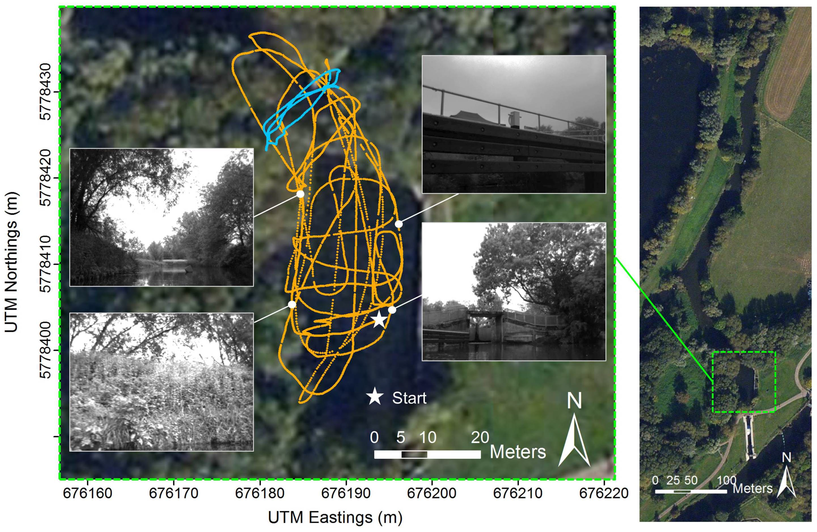
2.1. Case Study Site
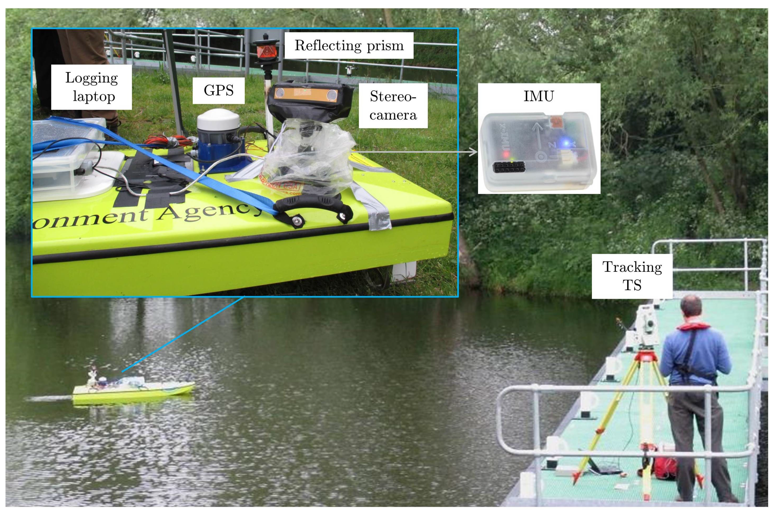
2.2. Data Collection

2.3. Visual Odometry
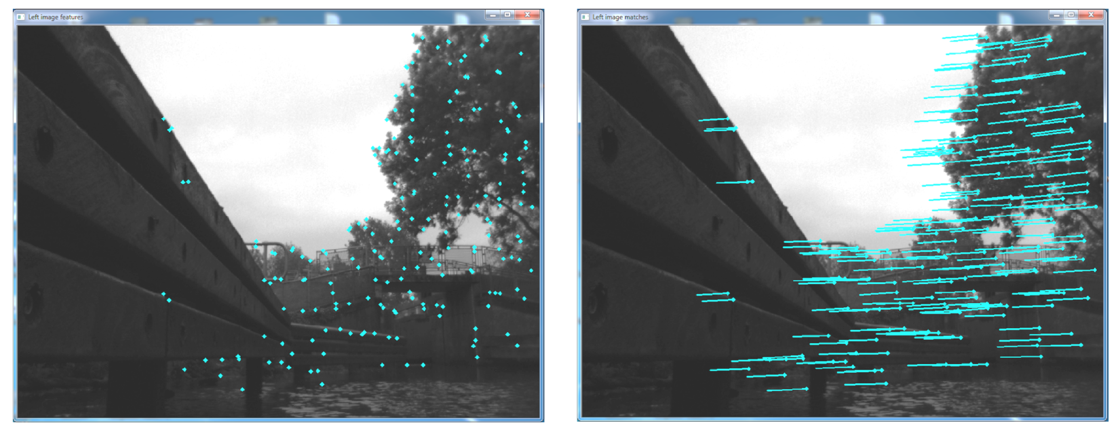
2.3.1. Using Sparse Features
- (i)
- (ii)
- (iii)
- extraction of the 3D real-world position P of feature points in as:where X, Y and Z are the real-world coordinates relative to the camera reference frame in meters, and are the coordinates of the feature points in the image domain, and are the coordinates of the image centre along the optical axis, f is the focal length of the camera in pixels, B is the stereo baseline in meters and D is the pixel disparity of feature pairs matched between and ; and
- (iv)
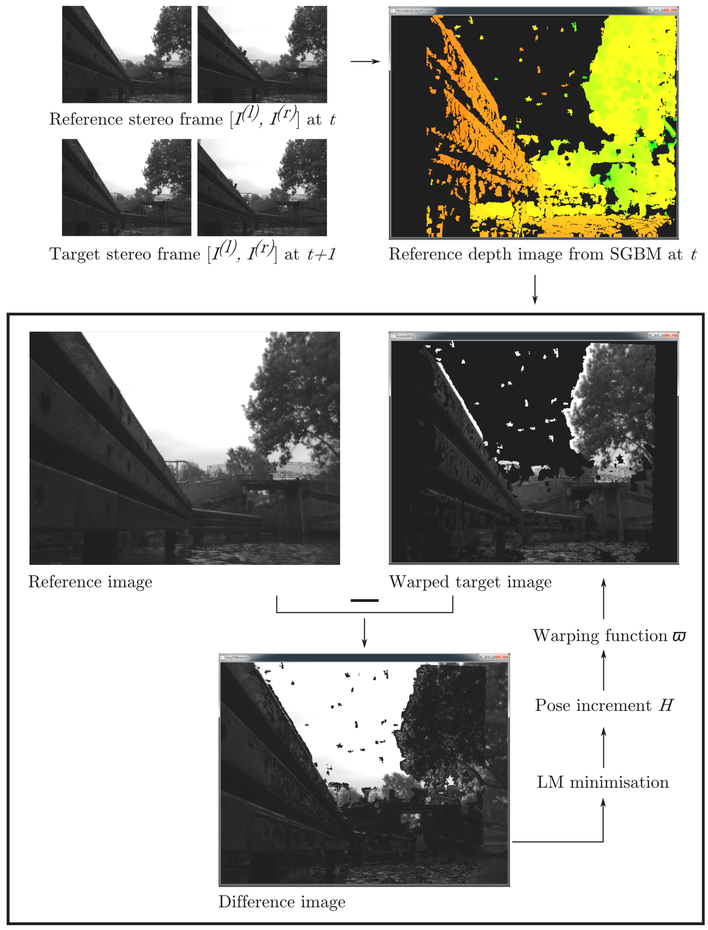
- estimation of the rotation R and translation T, describing the incremental camera motion by iteratively minimising the re-projection error e of the extracted 3D feature points into the 2D space of using Gauss–Newton optimisation, with:whereby here, and are the feature locations in the left and right current images, respectively, and and denote the projection from 3D to 2D space.

2.3.2. Using Dense Features

2.4. Validation
- v: the section mean of total vessel speed (in ms−1), quantified as distance travelled over time based on the Total Station measurements;
- h: the section variability in platform yaw (in deg), quantified as the standard deviation of the platform yaw measured by the IMU;
- f: the section mean number of inlier feature matches (for sparse visual odometry) or the number of pixels with valid depth information (for dense visual odometry); and
- d: the section mean depth (in m) of matched inlier features (for sparse visual odometry) or the mean depth of pixels with valid depth information (for dense visual odometry).
3. Results and Discussion
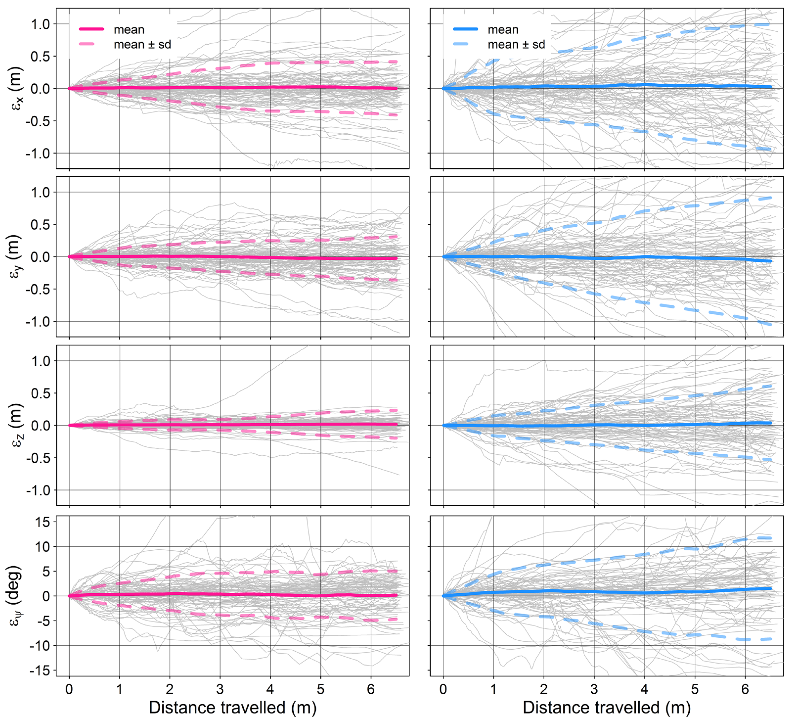
3.1. Error Statistics

| Min | Mean | Median | SD | Max | n | ||
|---|---|---|---|---|---|---|---|
| sparse | 0.004 | 0.067 | 0.048 | 0.060 | 0.345 | ||
| −0.197 | 0.001 | −0.003 | 0.064 | 0.229 | |||
| −0.180 | −0.002 | −0.005 | 0.054 | 0.209 | |||
| −0.117 | 0.002 | 0.002 | 0.033 | 0.263 | |||
| −4.16 | −0.01 | 0.07 | 1.39 | 3.87 | |||
| −3.95 | 0.00 | 0.03 | 1.25 | 3.13 | |||
| −3.44 | 0.03 | 0.13 | 0.70 | 2.24 | 96 | ||
| dense | 0.007 | 0.177 | 0.139 | 0.149 | 0.757 | ||
| −0.563 | 0.002 | −0.002 | 0.151 | 0.564 | |||
| −0.755 | −0.010 | −0.002 | 0.152 | 0.505 | |||
| −0.366 | 0.005 | −0.000 | 0.089 | 0.278 | |||
| −7.10 | −0.14 | −0.14 | 2.84 | 6.54 | |||
| −8.48 | 0.10 | 0.05 | 2.94 | 8.46 | |||
| −5.27 | 0.23 | 0.40 | 1.51 | 4.20 | 92 |

| 3D | 2D | |||||
|---|---|---|---|---|---|---|
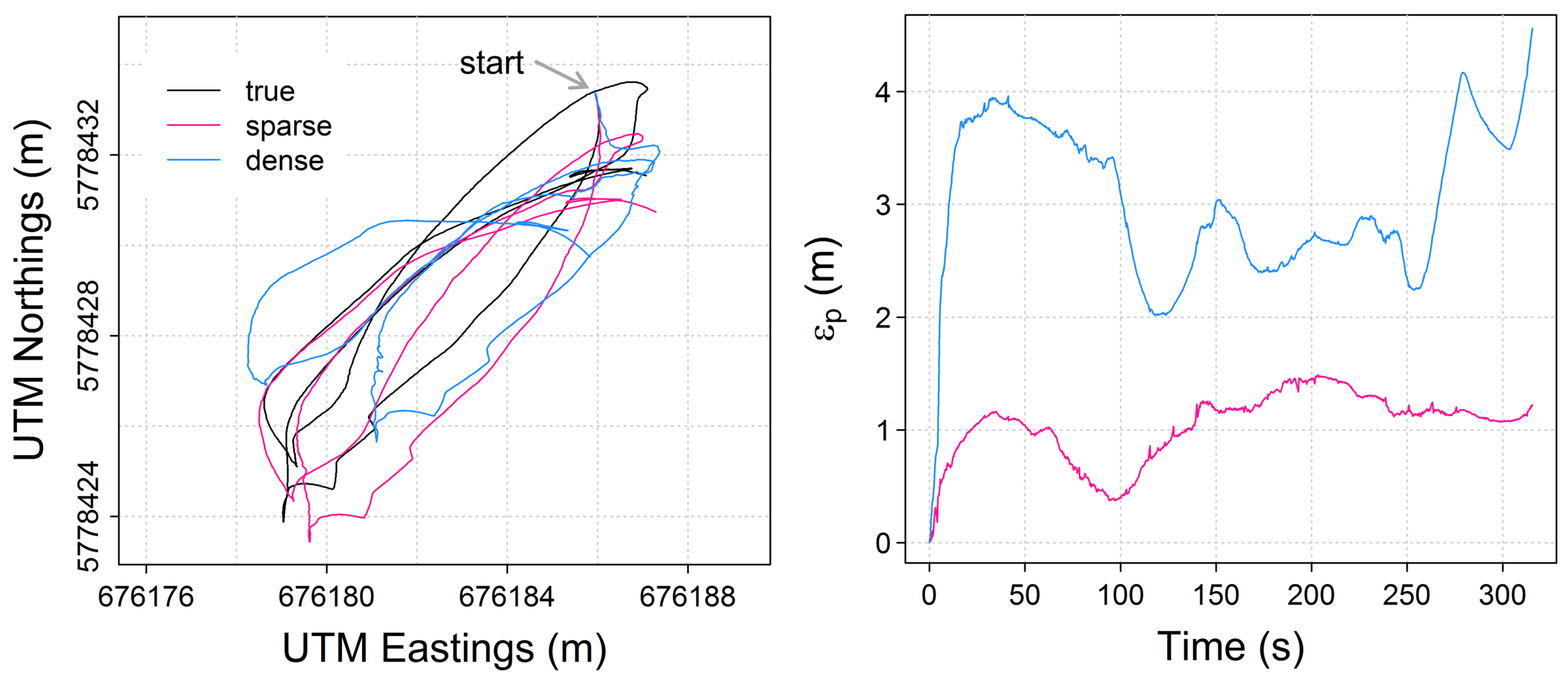
| Discharge measurement | sparse | 1.08 (1.99) | 1.51 (2.80) | 0.83 (1.54) | 1.21 (2.25) | |
| dense | 3.10 (5.74) | 4.56 (8.44) | 1.94 (3.58) | 3.08 (5.69) | 1265 | |
| Total trajectory | sparse | 13.36 (2.01) | 25.01 (3.77) | 9.56 (1.44) | 18.03 (2.72) | |
| dense | 31.49 (4.75) | 65.43 (9.87) | 21.53 (3.25) | 56.83 (8.57) | 7491 |


3.2. Effects of Platform Kinematics and Scenery
| β | t | p-Value (t) | F | p-Value (F) | R | ||
|---|---|---|---|---|---|---|---|
| sparse | e | 0.82 | 0.42 | ||||
| v | 5.22e | 0.04 | 0.97 | ||||
| h | 2.33e | 9.53 | 0.00 * | ||||
| f | 6.84e | 1.12 | 0.27 | ||||
| d | 1.46e | 2.73 | 0.01 * | 28.70 | 0.00 * | 0.56 | |
| dense | e | −0.20 | 0.85 | ||||
| v | 1.24e | 2.06 | 0.04 * | ||||
| h | 1.39e | 1.24 | 0.22 | ||||
| f | e | −0.43 | 0.67 | ||||
| d | 9.84e | 3.52 | 0.00 * | 7.10 | 0.00 * | 0.25 |
| Min | Mean | Median | SD | Max | n | ||
|---|---|---|---|---|---|---|---|
| sparse | v (ms) | 0.10 | 0.57 | 0.53 | 0.37 | 1.49 | |
| h (deg) | 0.33 | 17.42 | 10.45 | 18.37 | 75.08 | ||
| f | 40 | 233 | 238 | 90 | 422 | ||
| d (m) | 4.13 | 21.60 | 20.53 | 9.30 | 39.38 | 96 | |
| dense | v (ms) | 0.10 | 0.56 | 0.53 | 0.35 | 1.42 | |
| h (deg) | 0.33 | 17.79 | 11.13 | 18.48 | 75.08 | ||
| f | 306,400 | 540,700 | 568,000 | 88,598 | 656,400 | ||
| d (m) | 6.13 | 20.75 | 20.03 | 7.90 | 36.85 | 92 |
3.3. Implications for Autonomous River Monitoring
4. Conclusions
Acknowledgements
Author Contributions
Conflicts of Interest
References
- Dunbabin, M.; Marques, L. Robotics for Environmental Monitoring: Significant Advancements and Applications. IEEE Robot. Autom. Mag. 2012, 19, 24–39. [Google Scholar] [CrossRef]
- European Commission (EC). Directive 2000/60/EC of the Parliament and of the Council Establishing a Framework for Community Action in the Field of Water Policy. Off. J. Eur. Commun. 2000, L327, 1–72. [Google Scholar]
- European Commission (EC). Council Regulation (EC) No 1100/2007 of 18 September 2007 Establishing Measures for the Recovery of the Stock of European Eel. Off. J. Eur. Union 2007, L248, 17–23. [Google Scholar]
- Mueller, D.S.; Wagner, C.R.; Rehmel, M.; Oberg, K.A.; Rainville, F. Measuring Discharge with Acoustic Doppler Current Profilers from a Moving Boat. Techniques and Methods 3-A22, Version 2.0; Technical Report; United States Geological Survey (USGS): Reston, VA, USA, 2013.
- Kriechbaumer, T.; Blackburn, K.; Everard, N.; Rivas-Casado, M. Acoustic Doppler Current Profiler Measurements Near a Weir with Fish Pass: Assessing Solutions to Compass Errors, Spatial Data Referencing and Spatial Flow Heterogeneity. Hydrol. Res. 2015. [Google Scholar] [CrossRef]
- Dinehart, R.; Burau, J. Repeated Surveys by Acoustic Doppler Current Profiler for Flow and Sediment Dynamics in a Tidal River. J. Hydrol. 2005, 314, 1–21. [Google Scholar] [CrossRef]
- Environment Agency. National Standard Contract and Specification for Surveying Services. Version 3.2; Technical Report; Environment Agency: Bristol, UK, 2013. [Google Scholar]
- Queensland Government. Standards for Hydrographic Surveys Within Queensland Waters. Revision 1.3; Technical Report; Queensland Government: Collinsville, Australia, 2009.
- Wagner, C.R.; Mueller, D.S. Comparison of Bottom-Track to Global Positioning System Referenced Discharges Measured Using an Acoustic Doppler Current Profiler. J. Hydrol. 2011, 401, 250–258. [Google Scholar] [CrossRef]
- Fuentes-Pacheco, J.; Ruiz-Ascencio, J.; Rendón-Mancha, J.M. Visual Simultaneous Localization and Mapping: A Survey. Artif. Intell. Rev. 2015, 43, 55–81. [Google Scholar] [CrossRef]
- Casado, R.M.; Gonzalez, B.R.; Kriechbaumer, T.; Veal, A. Automated Identification of River Hydromorphological Features Using UAV High Resolution Aerial Imagery. Sensors 2015, 15, 27969–27989. [Google Scholar] [CrossRef] [PubMed] [Green Version]
- Flynn, K.; Chapra, S. Remote Sensing of Submerged Aquatic Vegetation in a Shallow Non-turbid River Using an Unmanned Aerial Vehicle. Remote Sens. 2014, 6, 12815–12836. [Google Scholar] [CrossRef]
- Nistér, D.; Naroditsky, O.; Bergen, J. Visual Odometry. In Proceedings of the 2004 IEEE Computer Society Conference on Computer Vision and Pattern Recognition (CVPR 2004), Washington, DC, USA, 27 June–2 July 2004; pp. 652–659.
- Moravec, H.P. Obstacle Avoidance and Navigation in the Real World by a Seeing Robot Rover. Ph.D. Thesis, Carnegie-Mellon University, Pittsburgh, PA, USA, 1980. [Google Scholar]
- Scaramuzza, D.; Fraundorfer, F. Visual Odometry. Part I: The First 30 Years and Fundamentals. IEEE Robot. Autom. Mag. 2011, 18, 80–92. [Google Scholar] [CrossRef]
- Koletschka, T.; Puig, L.; Daniilidis, K. MEVO: Multi-Environment Stereo Visual Odometry. In Proceedings of the 2014 IEEE/RSJ International Conference on Intelligent Robots and Systems (IROS 2014), Chicago, IL, USA, 14–18 September 2014; pp. 4981–4988.
- Konolige, K.; Agrawal, M.; Sol, J. Large Scale Visual Odometry for Rough Terrain. In Proceedings of the 13th International Symposium of Robotics Research, Hiroshima, Japan, 26–29 November 2007.
- Fischler, M.A.; Bolles, R.C. Random Sample Consensus: A Paradigm for Model Fitting with Applications to Image Analysis and Automated Cartography. Commun. ACM 1981, 24, 381–395. [Google Scholar] [CrossRef]
- Magnabosco, M.; Breckon, T.P. Cross-Spectral Visual Simultaneous Localization and Mapping (SLAM) with Sensor Handover. Robot. Autonom. Syst. 2013, 61, 195–208. [Google Scholar] [CrossRef]
- Warren, M.; Mckinnon, D.; He, H.; Upcroft, B. Unaided Stereo Vision Based Pose Estimation. In Proceedings of the Australasian Conference on Robotics and Automation, Brisbane, Australia, 1–3 December 2010.
- Geiger, A.; Ziegler, J.; Stiller, C. StereoScan: Dense 3D Reconstruction in Real-Time. In Proceedings of the IEEE Intelligent Vehicles Symposium (IV), Baden-Baden, Germany, 5–9 June 2011; pp. 963–968.
- Lemaire, T.; Berger, C.; Jung, I.K.; Lacroix, S. Vision-Vased SLAM: Stereo and Monocular Approaches. Int. J. Comput. Vis. 2007, 74, 343–364. [Google Scholar] [CrossRef]
- Kitt, B.; Geiger, A.; Lategahn, H. Visual Odometry Based on Stereo Image Sequences with RANSAC-Based Outlier Rejection Scheme. In Proceedings of the IEEE Intelligent Vehicles Symposium (IV), San Diego, CA, USA, 21–24 June 2010; pp. 486–492.
- Konolige, K.; Bowman, J.; Chen, J.D.; Mihelich, P.; Calonder, M.; Lepetit, V.; Fua, P. View-Based Maps. Int. J. Robot. Res. 2010, 29, 941–957. [Google Scholar] [CrossRef]
- Grimes, M.; LeCun, Y. Efficient Off-Road Localization Using Visually Corrected Odometry. In Proceedings of the IEEE International Conference on Robotics and Automation (ICRA ’09), Kobe, Japan, 12–17 May 2009; pp. 2649–2654.
- Maimone, M.; Cheng, Y.; Matthies, L. Two Years of Visual Odometry on the Mars Exploration Rovers. J. Field Robot. 2007, 24, 169–186. [Google Scholar] [CrossRef]
- Steinbrucker, F.; Sturm, J.; Cremers, D. Real-Time Visual Odometry From Dense RGB-D Images. In Proceedings of the IEEE International Conference on Computer Vision Workshops (ICCV Workshops), Barcelona, Spain, 6–13 November 2011.
- Audras, C.; Comport, A.; Meilland, M.; Rives, P. Real-Time Dense Appearance-based SLAM for RGB-D Sensors. In Proceedings of the Australian Conference on Robotics and Automation (ACRA), Melbourne, Australia, 7–9 December 2011.
- Kerl, C.; Sturm, J.; Cremers, D. Robust Odometry Estimation for RGB-D Cameras. In Proceedings of the IEEE International Conference on Robotics and Automation (ICRA), Karlsruhe, Germany, 6–10 May 2013; pp. 3748–3754.
- Engel, J.; Sturm, J.; Cremers, D. Semi-Dense Visual Odometry for a Monocular Camera. In Proceedings of the IEEE International Conference on Computer Vision (ICCV), Sydney, Australia, 1–8 December 2013; pp. 1449–1456.
- Comport, A.I.; Malis, E.; Rives, P. Accurate Quadrifocal Tracking for Robust 3D Visual Odometry. In Proceedings of the IEEE International Conference on Robotics and Automation, Rome, Italy, 10–14 April 2007; pp. 40–45.
- Comport, A.I.; Malis, E.; Rives, P. Real-Time Quadrifocal Visual Odometry. Int. J. Robot. Res. 2010, 29, 245–266. [Google Scholar] [CrossRef] [Green Version]
- Yang, J.; Rao, D.; Chung, S.J.; Hutchinson, S. Monocular Vision Based Navigation in GPS-Denied Riverine Environments. In Proceedings of the AIAA Infotech@ Aerospace Conference, St. Louis, MO, USA, 29–31 March 2011; pp. 1–12.
- Chambers, A.; Achar, S.; Nuske, S.; Rehder, J.; Kitt, B.; Chamberlain, L.; Haines, J.; Scherer, S.; Singh, S. Perception for a River Mapping Robot. In Proceedings of the IEEE/RSJ International Conference on Intelligent Robots and Systems (IROS), San Francisco, CA, USA, 25–30 September 2011; pp. 227–234.
- Scherer, S.; Rehder, J.; Achar, S.; Cover, H.; Chambers, A.; Nuske, S.; Singh, S. River Mapping From a Flying Robot: State Estimation, River Detection, and Obstacle Mapping. Auton. Robot. 2012, 33, 189–214. [Google Scholar] [CrossRef]
- Rehder, J.; Gupta, K.; Nuske, S.; Singh, S. Global Pose Estimation with Limited GPS and Long Range Visual Odometry. In Proceedings of the IEEE International Conference on Robotics and Automation (ICRA), Saint Paul, MN, USA, 14–18 May 2012; pp. 627–633.
- Fang, Z.; Zhang, Y. Experimental Evaluation of RGB-D Visual Odometry Methods. Int. J. Adv. Robot. Syst. 2015, 12, 1–16. [Google Scholar] [CrossRef]
- Petrie, J.; Diplas, P.; Gutierrez, M.; Nam, S. Combining Fixed- and Moving-Vessel Acoustic Doppler Current Profiler Measurements for Improved Characterization of the Mean Flow in a Natural River. Water Resour. Res. 2013, 49, 5600–5614. [Google Scholar] [CrossRef]
- Geiger, A.; Lenz, P.; Urtasun, R. Are We Ready for Autonomous Driving? The KITTI Vision Benchmark Suite. In Proceedings of the IEEE Conference on Computer Vision and Pattern Recognition (CVPR), Providence, RI, USA, 16–21 June 2012; pp. 3354–3361.
- Flener, C.; Wang, Y.; Laamanen, L.; Kasvi, E.; Vesakoski, J.M.; Alho, P. Empirical Modeling of Spatial 3D Flow Characteristics Using a Remote-Controlled ADCP System: Monitoring a Spring Flood. Water 2015, 7, 217–247. [Google Scholar] [CrossRef]
- HR Wallingford. ARC-Boat. Available online: http://www.hrwallingford.com/expertise/arc-boat (accessed on 8 June 2015).
- Point Grey Research. Bumblebee2 1394a. Available online: http://goo.gl/FsjDc4 (accessed on 8 June 2015).
- Madgwick, S.O.H.; Harrison, A.J.L.; Vaidyanathan, R. Estimation of IMU and MARG Orientation Using a Gradient Descent Algorithm. In Proceedings of the IEEE International Conference on Rehabilitation Robotics (ICORR), Zurich, Switzerland, 29 June–1 July 2011; pp. 1–7.
- X-IO Technologies. X-IMU. Available online: http://www.x-io.co.uk/products/x-imu/ (accessed on 8 June 2015).
- Leica Geosystems. Leica Viva TS15. Available online: http://goo.gl/p7zFlf (accessed on 8 June 2015).
- Bayoud, F.A. Leica’s Pinpoint EDM Technology with Modified Signal Processing and Novel Optomechanical Features. In Proceedings of the XXII FIG Congress: Shaping the Change, Munich, Germany, 8–13 October 2006; pp. 1–16.
- Kirschner, H.; Stempfhuber, W. The Kinematic Potential of Modern Tracking Total Stations—A State of the Art Report on the Leica TPS1200+. In Proceedings of the 1st International Conference on Machine Control & Guidance, Zurich, Switzerland, 24–26 June 2008.
- Horn, B.K.P. Closed-Form Solution of Absolute Orientation Using Unit Quaternions. J. Opt. Soc. Am. A 1987, 4, 629–642. [Google Scholar] [CrossRef]
- Hirschmuller, H. Stereo Processing by Semiglobal Matching and Mutual Information. IEEE Trans. Pattern Anal. Mach. Intell. 2008, 30, 328–341. [Google Scholar] [CrossRef] [PubMed]
- Neubeck, A.; van Gool, L. Efficient Non-Maximum Suppression. In Proceedings of the 18th International Conference on Pattern Recognition (ICPR 2006), Hong Kong, China, 20–24 August 2006; pp. 850–855.
- Thrun, S.; Burgard, W.; Fox, D. Probabilistic Robotics; MIT Press: Cambridge, MA, USA, 2005; p. 672. [Google Scholar]
- Mroz, F.; Breckon, T.P. An Empirical Comparison of Real-Time Dense Stereo Approaches for Use in the Automotive Environment. EURASIP J. Image Video Proc. 2012, 13, 1–19. [Google Scholar] [CrossRef] [Green Version]
- Sokal, R.R. Biometry: The Principles and Practices of Statistics in Biological Research, 3rd ed.; W.H.Freeman and Co.: New York, NY, USA, 1994; p. 880. [Google Scholar]
- Zhao, J.; Chen, Z.; Zhang, H. A Robust Method for Determining the Heading Misalignment Angle of GPS Compass in ADCP Measurement. Flow Meas. Instrum. 2014, 35, 1–10. [Google Scholar] [CrossRef]
- Zhang, H.; Liu, Y.; Tan, J. Loop Closing Detection in RGB-D SLAM Combining Appearance and Geometric Constraints. Sensors 2015, 15, 14639–14660. [Google Scholar] [CrossRef] [PubMed]
- Cummins, M.; Newman, P. Appearance-only SLAM at Large Scale with FAB-MAP 2.0. Int. J. Robot. Res. 2011, 30, 1100–1123. [Google Scholar] [CrossRef]
- Hamilton, O.K.; Breckon, T.P.; Bai, X.; Kamata, S.I. A Foreground Object Based Quantitative Assessment of Dense Stereo Approaches for Use in Automotive Environments. In Proceedings of the 20th IEEE International Conference on Image Processing (ICIP), Melbourne, Australia, 15–18 September 2013; pp. 418–422.
- Jamieson, E.C.; Ruta, M.A.; Rennie, C.D.; Townsend, R. Monitoring Stream Barb Performance in a Semi-Alluvial Meandering Channel: Flow Field Dynamics and Morphology. Ecohydrology 2013, 6, 611–626. [Google Scholar] [CrossRef]
- Rennie, C.D.; Rainville, F. Case Study of Precision of GPS Differential Correction Strategies: Influence on aDcp Velocity and Discharge Estimates. J. Hydraul. Eng. 2006, 132, 225–234. [Google Scholar] [CrossRef]
- Kaneko, K.; Nohara, S. Review of Effective Vegetation Mapping Using the UAV (Unmanned Aerial Vehicle) Method. J. Geogr. Inf. Syst. 2014, 6, 733–742. [Google Scholar] [CrossRef]
© 2015 by the authors; licensee MDPI, Basel, Switzerland. This article is an open access article distributed under the terms and conditions of the Creative Commons by Attribution (CC-BY) license (http://creativecommons.org/licenses/by/4.0/).
Share and Cite
Kriechbaumer, T.; Blackburn, K.; Breckon, T.P.; Hamilton, O.; Rivas Casado, M. Quantitative Evaluation of Stereo Visual Odometry for Autonomous Vessel Localisation in Inland Waterway Sensing Applications. Sensors 2015, 15, 31869-31887. https://doi.org/10.3390/s151229892
Kriechbaumer T, Blackburn K, Breckon TP, Hamilton O, Rivas Casado M. Quantitative Evaluation of Stereo Visual Odometry for Autonomous Vessel Localisation in Inland Waterway Sensing Applications. Sensors. 2015; 15(12):31869-31887. https://doi.org/10.3390/s151229892
Chicago/Turabian StyleKriechbaumer, Thomas, Kim Blackburn, Toby P. Breckon, Oliver Hamilton, and Monica Rivas Casado. 2015. "Quantitative Evaluation of Stereo Visual Odometry for Autonomous Vessel Localisation in Inland Waterway Sensing Applications" Sensors 15, no. 12: 31869-31887. https://doi.org/10.3390/s151229892