2.1. Feature Extraction from Original Response Curves
The first feature extraction method is to extract piecemeal signal features from the original response curves of sensors, including steady-state response and transient responses such as maximum value, integrals, derivatives, area values, rising time, falling time, rising slopes, falling slopes,
etc. Because the maximum value represents the final steady-state feature of the entire dynamic response process in the final balance, which reflects the maximum reaction degree change of sensors responding to odors, it is usually used as the most common and simple E-nose feature. In the early stages of the published history of E-noses, transient information was not used in sensor signal feature extraction. A variety of steady-state models (maximum value) have been used as feature extraction method for gas sensor signals, as illustrated in
Table 1.
Table 1.
Some maximum value feature models.
Table 1.
Some maximum value feature models.
| Model | Description | References |
|---|
| Difference | | [42] |
| Relative difference | | [43] |
| Fractional difference | | [44] |
| Logarithm difference | | [45] |
| Sensor normalization | | [45,46] |
| Array normalization | | [47,48] |
and
represent the processed maximum value feature and the original maximum response value of the of the
i-th sensor to the
j-th gas, respectively. The difference method can usually eliminate the additive errors, which are added both to the baseline and the steady-state response (meaning the response of the
i-th sensor to the
j-th gas). There is some evidence that the relative and fractional difference are helpful to compensate for the temperature influence on the sensors and the fractional difference linearizes the mechanism that generates a concentration dependence in metal oxide chemiresistor sensors [
47]. The log difference is more suitable when the variation of the concentration of the odor is very large because it is able to linearize the highly nonlinear relationship between odor concentration and the sensor output. The normalization models, which limit each sensor output between 0 and 1, thereby keep each element of the response vector at the same magnitude. Not only can it reduce the calculation error of stoichiometric recognition, but also is very effective when it is not the odor concentration which is of interest, but rather the precise identification of the odor. This method for example provides good recognition results for the discrimination of several types of coffee using neural networks [
48].
Besides the steady-state features of response curves, various other transient features such as derivatives and integrals of original response curves were taken into research in many special applications. Balasubramanian
et al. used a MOS-based E-nose system, which was designed and fabricated at the Bio-Imaging and Sensing Center, North Dakota State University (Fargo, ND, USA) to analyze the headspace from beef strip loins stored at 4 °C and 10 °C. The designed system consisted of a cylindrical sampling chamber made of Teflon on to which seven thick film MOS (Figaro USA Inc., Glenview, IL, USA) and one integrated sensor sensitive to temperature and relative humidity (Sensirion AG, Zurich, Switzerland) were mounted at regular intervals. The headspace gas from the meat packages was drawn into the chamber using a diaphragm-type air pump, and a fan and valve assembly fixed at the bottom of the sample chamber facilitated purging the sensor array after analysis. Six areas features under the response curves were extracted from six gas sensors (TGS 812, TGS 822, TGS 880, TGS 2602, TGS 2611-1 and TGS 2611-2). Another four features were extracted from the remaining two sensors related to the relative humidity (RH), temperature and carbon dioxide readings. The results showed that the MOS-based electronic system integrated with radial basis function neural networks (RBFNN) obtained above 90% total maximum classification accuracy in identifying spoiled meat samples from the unspoiled meat samples with six area features and four additional environmental features for the meat samples stored at 4 °C and 10 °C [
49].
Distante
et al., used a homemade E-nose consisting of five SnO
2 sensors prepared by means of sol-gel technology with Pd, Pt, Os, and Ni as doping elements. The film thickness was 100 nm and the films were deposited on alumina substrates supplied with interdigitated electrodes and platinum heater, by the spin coating technique at 3000 rpm, dried at 80 °C and heat treated in air at 600 °C. After deposition, the sensors were mounted onto a TO8 socket and inserted in a test chamber. Three volatile organic compounds (VOCs) were investigated: acetone, hexanal and pentanone in 50% relative humidity (RH) and dry air. Several feature extraction methods, both steady-state feature maximum value and transient feature, were considered. The results showed that integral and derivatives methods have higher recognition rates than that of maximum values and they also concluded that the desorption stage is more informative than the adsorption stage of the original response curves [
50].
Roussel
et al., applied a homemade E-nose to discriminate satisfactory wines and unsatisfactory vinegar flavour wines. The measurement device is a metal oxide gas sensor array containing five Figaro TGS series SnO
2 sensors (TGS 800, 822, 824, 825 and 842) and modified to host a thermo-hygrometer and to acquire the sensor voltage on a 12 bit A/D converter. Twenty-nine features are extracted from each sensor response curve including seven mean response values on different time intervals, six slopes on different time intervals, eight primary derivatives and eight secondary derivatives. And then these features have been validated and evaluated qualitatively by three specific indexes: the repeatability, discrimination and redundancy. However, the authors just proposed the three indexes to qualitatively analyze the features but did not give any classification results for specific data using different features, which were considered better than others according to their proposed three evaluating indexes [
51].
Llobet
et al. established an array to discriminate between and quantify ethanol, toluene and
o-xylene at concentration ranges from 25 ppm to 100 ppm, which consisted of four commercially available Taguchi gas sensors: two TGS822, one TGS813 and one TGS800. The model TGS822 exhibits high sensitivity to alcohol and organic solvents. The model TGS813 is mainly sensitive to general combustible gases and the model TGS800 is sensitive to gasoline exhaust and other air contaminants. The steady-state feature (conductance change
) and conductance rise time (Tr, measured from 20% to 60% of
) were extracted as features and they found that the using Tr as feature gave much better qualitative recognition results and using
and Tr as features results in equal quantitative recognition rates, as shown in
Table 2, which meant that Tr was concentration-independent [
26].
Table 2.
Classification rates (CR) of different features in [
26].
Table 2.
Classification rates (CR) of different features in [26].
| Features | Qualitative CR (%) | Quantitative CR (%) |
|---|
| Difference maximum value | 66.7 | 95 |
| Conductance rise time Tr | 92 | 95 |
Eklöv
et al., investigated the concentration of gas mixtures of hydrogen and ethanol with a homemade E-nose with four platinum MOSFET sensors, which had a thin discontinuous platinum film covered gate oxide. The gate voltages of each MOSFET sensor were detected and the sampling frequency was set at 1 Hz. All measurements consisted of an absorption stage for 2 min and a desorption stage for 8 min with a flow rate of 100 mL/min. A sequence of different concentrations of hydrogen and ethanol that ranged between 0 and 50 ppm were tested. The extracted features could be divided into two types: simple parameters from the original response curves and coefficients from different curve fitting models. It is necessary to select these parameters systematically and take into consideration the noise properties as well as the relationship between the features and the recognition ability of the features in a specific problem [
52]. The features extracted from original response curves are shown in
Table 3. Several combinations of features were proposed and gave satisfactory concentration prediction results.
Table 3.
Description of features extracted from original response curves in [
52].
Table 3.
Description of features extracted from original response curves in [52].
| Parameters | Description |
|---|
| Baseline | |
| Final response, response | Sensor value (averaged over 5 s) at gasOffbaseline |
| 30/90 s on/off response | Sensor value (averaged over 5 s) 30/90 s after gasOn/Off—baseline |
| Maximum response | Max(sensor value)—baseline |
| Min/max derivative | Min/max difference between two samples during measurement |
| On/off derivative | (Sensor value 10 s after gasOn/Off−baseline)/10 |
| Plateau derivative | (Response90 s on response)/30 |
| Derivative | |
| Off integral | |
| Short on/off integral | |
| Response/on integral | Response/on integral |
| T0-90% | Time from gasOn for sensor value to reach baseline + 0.9 × response |
| T0-60% | Time from gasOn for sensor value to reach baseline + 0.6 × response |
| T100-10% | Time from gasOff for sensor value to reach baseline + 0.1 × response |
| T100-40% | Time from gasOff for sensor value to reach baseline + 0.4 × response |
These parameters can be assessed according to the signal to noise ratio (SNR), correlation and significance in a 2-dimensional PCA plot. The signal to standard deviation ratio (
) [
52], defined in Equation (1), was used to estimate the property of the features. It can provide similar information as a SNR:
In addition, principal component analysis (PCA) was used to analyze the features. The PCA result gave score plots and loading plots. The trends, groups and outliers of the samples can be observed in score plots and the correlation and similarity between the features can be observed. A longer distance from the origin in the loading plot and a larger SNR implied that the feature contained more information. The artificial neural networks (ANN) classification results showed that: (1) a large error is obtained only with the final response features; (2) it was possible to improve the prediction accuracy to use features according to the calculation; (3) there was information which can improve the recognition ability in the loading plot; (4) features extracted from original response curves may gave comparable results as the complex curve fitting coefficients; (5) there was more information about the detected materials in the shape of the whole response than only the response value.
Zhang
et al. used an array of six TGS gas sensors to detect four common flammable liquids (gasoline, kerosene, diesel oil and ethanol) and three incombustible drinks (ice black tea, orange juice and Coca Cola) in less than 10 s for each recognition. Because they needed to realize fast recognition with an E-nose, they must extract robust information from the first few seconds of the sensor response curves as less redundant as possible. They researched four features (integrals, differences, primary derivatives and secondary derivatives) at a specific interval from the original response curves to classification [
53]. Because integrals, differences, primary derivatives and secondary derivatives of the response curves are continuous with the interval changes, different positions of the curves can contain different information, which may consecutively change with the interval changes. Therefore, a calculating process was applied to fix at which interval of the response curves robust information can be extracted
St shown in Equation (2), was use to evaluated the information quality of the feature extracted at the time
t of the response curves from the sensor array, which is a criterion to measure the separative degree among different classes of data based on the scatter matrix [
54]. The expression of
St is:
where Sw
t is the scatter matrix within a class, while
is the scatter matrix among different classes. PCA and discriminant function analysis (DFA) results showed that 85.7% classification rate was obtained with the four features in optimal time
t, while only 57.1% classification rate was obtained with the maximum value feature.
Šetkus
et al., applied a homemade E-nose with s metal oxide (MOX) sensors array that contained commercial- and laboratory-made sensors to investigate some volatile organic compounds (VOCs), namely acetone, acetic acid, butyric acid, and acetaldehyde. The sensor array included two TGS type sensors (TGS2602, TGS2610). The laboratory-made sensors were based on tin oxide thin films, which were modified by catalytic metals such as Au, Pt, Pd and Ru, and were grown by rheotaxial (fused metal) growth and the thermal oxidation technique (RGTO). The authors researched three kinetic features: (1) the time the maximum value (τ
max); (2) the time interval between the beginning of the adsorption and the end of the transient signal; (3) the slope of the response calculated in the desorption stage. PCA results showed that the dynamic features added significant information and allowed a better discrimination of the VOCs than that of the relative maximum response value [
55].
Table 4.
Description of features extracted from original response curves in [
56].
Table 4.
Description of features extracted from original response curves in [56].
| Extracted Feature | Represent Meaning |
|---|
| Max slope | The respond rate of sensor to different vinegar gas |
| Maximum | The maximum respond value |
| Average of last 20 points | The stationary phase of equilibrium between reversible adsorption and desorption |
| Average of whole points | Sensor respond value during the whole process |
Zou
et al., used an E-nose based on five tin-oxide sensors from Figaro Co. Ltd. (TGS 813, TGS 880, TGS 822, TGS 825, TGS 812), one humidity sensor (HS-01) and one temperature sensor (Pt100) to identify two different types of vinegars. Four features are extracted from each curve, which are shown in
Table 4. They are the slope max, maximum, average of the last 20 points and the average of whole points of curve [
56]. In addition, an evaluation index, called “distinguish index” (DI), was proposed to evaluate the features.
Wei
et al., extracted the maximum values, area values and 70th s values as the features from the E-nose responses and the PCA results indicated that the 70th s values provided the most accurate results when classifying unshelled peanuts and peanut kernels, which could be distinguished reliably by using a two-dimensional PCA [
57].
From the above, many features can be extracted from original response curves (
Table 5). Some of the features have specific physical meanings and reflect different information of the reaction kinetics at different aspects. Maximum value represents the final steady-state feature of the entire dynamic response process in the final balance, reflecting the maximum reaction degree change of sensors responding to odors. Intervals may represent the accumulative total of the reaction degree changing and differences may represent the degree of the reaction. Primary derivatives (slopes) may represent the rate of the reaction of sensors responding to odors and secondary derivatives may represent the acceleration of the reaction,
etc. [
53,
58].
Table 5.
Summary of commonly used features extracted from original response curves
Table 5.
Summary of commonly used features extracted from original response curves
| Feature | Description | References |
|---|
| Maximum response | Max(sensor value) | [42,43,44,45,46,47,51,52,55,56,59] |
| Responses of special time | Response value of special time in the whole response curve | [51,52,56,57] |
| Time of special responses | Time of special response value in the whole response curve | [26,51,52,55] |
| Area | Area values of sensor response curve and time axis surrounded | [49,57] |
| Integral | | [50,52,53,59] |
| Derivative | | [50,51,52,53,56] |
| Difference | | [52,53,55,59] |
| Second derivative | | [51,53] |
By extracting these features we can get information about different aspects from the original reactions between the sensors and the odors. However, it is evident that which extraction methods from the original response curves are appropriate depends on the different sensors and applications and for different applications and sensors, the feature extraction methods which give the best features are different. Moreover, researchers are likely to use composite features because these types of features which usually contain steady-state and transient features can obtain better performance. It is not easy to draw a conclusion about which method is the best one. On the whole, for maximum features, the normalization models give better performance than the other models. The transient features can receive better recognition accuracy than that of the steady-state feature and especially integral methods generally give the best features for many different E-nose applications. Based on the previous researches, a summary is listed in
Table 5, which provides a brief description of the features commonly used in previous researches.
2.2. Features Extraction from Curve Fitting Parameters
Instead of extracting characteristics from the raw data curve, an alternative method is to model sensor response curves and then extract features based on the model coefficients. Curve fitting is a data processing method which approximately characterizes or analogizes the functional relationship of discrete points using continuous curves. The curve fitting method approximates discrete data using analytical expressions. The basic idea is to determine the fitting function in accordance with the trend of the discrete points. It utilizes the discrete points, but is not limited to these discrete points. In curve fitting, the critical and complex problem is how to select and envision the specific form of the unknown function.
There are two strict mathematical laws on theories to follow for curve fitting. However, two approaches are generally followed: (1) determine the basic type of function through the study of the physical concepts between the variables and deep understanding of professional knowledge and (2) determine the type of function through the observation of general trends of the curve of experimental data. The root mean square error (RMSE) for the validation data can be calculated for each curve fitting model and used to evaluate the effect of the curve fitting.
Polynomial function models are usually applied to fit a number of kinds of curves. The curve fitting and features extraction can be carried out on not only the adsorption or desorption parts of the response curves respectively, but also the entire response process. In polynomial functions model,
n-degree polynomials are used to fit the response curves:
During the adsorption part the response curves, y represents the sensor response value, x represents the time from gas on to gas off. During the desorption part of the response curves, y represents the final response value subtracting the sensor value, x represents the time from gas off to the end. The fitting model parameters A0, A1, A2, A3, ···, An are used as features.
Exponential function models which are expressed in Equation (4) are another common model in studies used to model E-nose response curves [
59]. When the number
N equals 1 or 2, the exponential function model is called single-exponential function model and double-exponential functions, which are the most commonly used exponential function models:
where
y and
x are defined as the same in the polynomial function model and the fitting model parameters
A0,
T1, ···,
TN are used as features.
Auto-Regressive with eXogenous variables (ARX) models are widely built to represent dynamic behavior, used for time series prediction and system identification, and used a different way from the former two types of methods. The combination of sensor and target gas can be regarded as a dynamic system, which gives a response when exposed to a step function. This type of system can be modeled using an ARX model. In [
52], not only are simple parameters from original response curves extracted as the features shown in
Table 3, but also coefficients from different curve fitting models are taken into consideration. Four models, third-order polynomial function, single-exponential functions, double-exponential functions and ARX model, shown in
Table 6, were applied to fit the response curves of E-nose and the corresponding fitting model parameters were extracted as features for recognition.
Table 6.
Description of features extracted from curve fitting models in [
52].
Table 6.
Description of features extracted from curve fitting models in [52].
| Parameters | Description |
|---|
| Polynomial on/off |
|
| Exponential on/off | , where y and x are defined as in the polynomial fit. |
| Exponential on/off | , where y and x are defined as in the polynomial fit. |
| ARX on/off | ,
On: y(t) = (sensor value − baseline), t time from gas on—5 s to gas off
u(t) = 0 if test gas off and 1 if test gas on
Off: y(t) = (maximum value − sensor value), t = time from gas off—5 s to end
u(t) = 1 if test gas off and 0 if test gas on |
Table 7 showed neural network prediction results for different features in [
52]. As expected, only using one feature, the final response gave a large error. It is possible to improve the prediction accuracies according to the information obtained from the
. On/off derivatives have higher S/a-ratios than max/min derivatives and short on/off integrals, and the prediction errors showed the same tendency than using final responses, so combined with on/off derivatives as features they can obtain lower errors than for the other two combinations (models 2–4 in
Table 7). Information from the PCA loading plot can be used to improve the prediction ability too. Final response, 30 s and 90 s on response, which all are adjacent in the loading plot gave worse prediction ability than that of final response together with 30 s and 90 s off response (models 5 and 6 in
Table 7), which are located farther. On the whole, the curve fitting model parameters for the entire curves gave worse results compared with the features extracted from original response curves, except for the polynomial coefficients, which can obtain equally good results. Hence, curve fitting parameter features, which refer to the whole response, cannot guarantee better recognition results than those of the simple and piecemeal features combination, which gives comparable results as the more complex curve fitting parameters if chosen carefully.
Carmel
et al. researched a large dataset composed of 30 volatile odorous substances using a MOSES II E-nose equipped with two sensor modules: an eight-sensor quartz-microbalance (QMB) module and, and an eight-sensor metal-oxide (MOX) module. The samples were put in 20 mL vials in a headspace sampler and the headspace contents were injected into the E-nose, first introduced into the QMB chamber and then the MOX chamber. The injection lasts for 30 s and then a 15 min desorption stage follows. In total, 300 measurements were collected with an average of 10 per chemical. The exponential model, Lorentzian model and double-sigmoid model were applied to fir a curve the response for feature extraction [
27].
Table 7.
Results of neural network estimation from different features in [
52].
Table 7.
Results of neural network estimation from different features in [52].
| Model | Features | ANN Architecture | RMSE for Validation (ppm) |
|---|
| 1 | Final response | 1-2-2 | 13.4 |
| 2 | Final response | 3-3-2 | 2.2 |
| On/off derivative |
| 3 | Final response | 3-3-2 | 2.6 |
| Min/max derivative |
| 4 | Final response | 3-3-2 | 3.6 |
| Short on/off integral |
| 5 | Final response | 3-3-2 | 4.5 |
| 30 s on response |
| 90 s on response |
| 6 | Final response | 3-3-2 | 2.4 |
| 30 s off response |
| 90 s off response |
| 7 | Final response | 5-4-2 | 1.6 |
| 30 s on/off response |
| 90 s on/off response |
| 8 | Final response | 5-4-2 | 1.7 |
| On/off derivative |
| on/off integral |
| 9 | Final response | 6-5-2 | 1.7 |
| On/off derivative |
| Plateau derivative |
| Response/on integral |
| 10 | Polynomial on/off | 8-6-2 | 1.6 |
| 11 | 1. Exponential on/off | 4-4-2 | 2.0 |
| 12 | 2. Exponential on/off | 10-6-2 | 2.1 |
| 13 | ARX on/off | 6-5-2 | 2.3 |
The Lorentzian model is derived from a simple physical description of the measurement process. It applies four parameters, with respective specific physical meaning, which can be obtained from a curve fitting process. The double-sigmoid model was also used for curve fitting. The model with nine parameters function had been constructed by multiplying a monotonically decreasing sigmoid function by a monotonically increasing one. The explicit form of Lorentzian model and double-sigmoid model are expressed in Equations (5) and (6), respectively, and the details of the parameters in the two equations are presented in [
27]:
where
t is the response time and
,
T is the whole response time,
ti is the time how long a particle of the investigated chemical makes its way between the inlet and sensor
i, which is just the time when the signal starts to rise. The parameters
ti,
T,
can be used as features.
where the parameters
can be used as features.
Table 8.
Classification rates (CR) of different feature sets for QMB or MOX modules in [
27].
Table 8.
Classification rates (CR) of different feature sets for QMB or MOX modules in [27].
| Classifiers | Modules | Feature Sets | CR (%) |
|---|
| k-Nearest Neighbor (with k = 3) | QMB | | 97.8 |
| 90 |
| 84.4 |
| 96.7 |
| Mahalanobis distance discrimination in four-dimensional PCA space | QMB | | 83.3 |
| 96.7 |
| 42.2 |
| 60 |
| k-Nearest Neighbor (with k = 5) | MOX | | 93.1 |
| 90 |
| 86.9 |
| 93.5 |
Fifty-one feature sets were tested and applied to 101 datasets with nine classifiers. The nine classifiers were based on two types of classifiers. A k-nearest-neighbors (k-NN) classifier [
60] with
, and classifier in the base of the shortest Mahalanobis distance discrimination [
60] in the 1 to 5 dimensional principal components spaces. Average classification performance was calculated and ranked for every feature sets and
Table 8 showed the classification performance of several feature sets in [
27]. From the ranking of the fifty-one feature sets, the best feature set was
, which meant classify by majority rule among
, which was the difference between the maximum value and its baseline, and the parameters of the Lorentzian model. The best non-majority feature set was
. On the whole, the Lorentzian model was better than the exponential model with respect to classification rate and they were both much better than the standard features, which classified by majority rule among
and the area beneath the curve, the area beneath the curve left of the peak, and the time it took for the signal to reach its maximum value. Among the three models investigated in [
27], the analysis results showed that among the three models (exponential function models, Lorentzian model and double-sigmoid model) with respect to goodness of fit, computation speed, robustness and classification rate, the Lorentzian model was the best model for feature extraction and the most potent set of features resulting in higher classification rates than other combinations of features was
. Some other models are also used to characterize E-nose measurements, such as models based on sigmoid function [
61], fractional function, arc tangent function, and hyperbolic tangent function [
62]. A summary of different curve fitting models is shown in
Table 9.
Table 9.
Summary of common used curve fitting models.
Table 9.
Summary of common used curve fitting models.
| Model | Description | References |
|---|
| Third-order polynomial function | | [52,62] |
| Single-exponential function | | [52,62] |
| Double-exponential function | | [52,62] |
| ARX model | | [52] |
| Lorentzian model | Equation (5) | [27] |
| Double-sigmoid model | Equation (6) | [27] |
| Sigmoid function | | [61] |
| Fractional function | | [62] |
| Arctangent function | | [62] |
| Hyperbolic tangent function | | [62] |
2.3. Features Extraction from Transform Domain
Another method to extract features for E-noses is based on some transforms and then the transform coefficients are used as features to discriminate materials. The most commonly used transforms in E-nose signal processing are the Fourier transform and wavelet transform.
The widely used Fourier transform, for which the basis functions are sine and cosine, maps the original data into a new space. It decomposes the original response into the superposition of the dc component and different harmonic components, and the feature characterized by amplitude of each component can be used for qualitative and quantitative analysis. However, the problem of using the Fourier transform is the impossibility of localizing frequencies in the time domain. This problem can be overcome if we can add the information about the localization of these frequencies in the time domain that can be addressed with the theory of wavelet transform. Wavelet transform [
63] is an extension of the Fourier transform. It maps the signals into a new space with basis functions quite localizable in time and frequency space. The wavelet transform decomposes the original response into the approximation (low frequencies) and details (high frequencies). It displays good anti-interference ability [
64] for the subsequent pattern recognition if one uses the wavelet coefficients of certain sub-bands as features. Unlike the Fourier transform, the shapes of components of the decomposed signal are different according to the different shapes of the using mother wavelet. The common types of wavelet are Haar wavelet, Daubechies wavelet, Symlet wavelet, Coiflets wavelet, Biorthogonal wavelet, Morlet wavelet, Gaussian wavelet, Mexican hat wavelet, Meyer wavelet, Morlet wavelet,
etc.
Jia
et al. [
62] constructed a gas sensor array with six metal oxide sensors and one electrochemical sensor and used it to detect the seven species of pathogen most common in wound infections:
P. aeruginosa,
E. coli,
Acinetobacter spp.,
S. aureus,
S. epidermidis,
K. pneumoniae, and
S. pyogenes. They researched and compared the effect of different features of sensors including maximum values, integrals, derivatives, six types of curve fitting model parameters, FFT coefficients and DWT coefficients. In this research, a Daubechies family wavelet (db
N) was used and the variant
N was the order of the wavelet. For the Daubechies family wavelet, the
N was the vanishing moment. A larger
N can result in stronger localization ability in the frequency domain and better frequency band allocation results, and then, the energy is more concentrated. The results showed that the selected FFT feature, the amplitudes of the DC component, and DWT feature, the mean of the approximating coefficients after decomposition of 12 levels with the sixth order Daubechies family wavelet (db6), can both achieve a 100% correct classification rate, shown in
Table 10, which is generally higher than that of the other features except for integral features, single-exponential function and hyperbolic tangent function fitting parameters, which can provide the same 100% correct classification rate.
Table 10.
Classification rates (CR) of three types of features in [
62].
Table 10.
Classification rates (CR) of three types of features in [62].
| Feature Type | Feature | CR (%) |
|---|
| Original response curve | Maximum | 94.29 |
| Integrals | 100 |
| Derivatives | 97.14 |
| Curve fitting parameters | Three-order polynomial function | 91.43 |
| Fractional function | 97.14 |
| Single-exponential function | 100 |
| Double-exponential function | 68.57 |
| Arctangent function | 91.43 |
| Hyperbolic tangent function | 100 |
| Transform domain | FFT | 100 |
| DWT | 100 |
Distante
et al. [
50] also analyzed and researched the effect of features of E-noses from original response curves and transform domains for the application to volatile organic compound detection. The results are shown in
Table 11. It is evident that the wavelet transform coefficients can obtain the highest classification rate and it is interesting to note that integrals method produces very informative features as compared with the results obtained with the wavelet descriptors.
Table 11.
Classification rates (CR) of different features in [
50].
Table 11.
Classification rates (CR) of different features in [50].
| Feature Type | Feature | CR (%) |
|---|
| Original response curve | Difference maximum | 83 |
| Relative maximum | 81 |
| Fractional maximum | 82 |
| Log maximum | 81 |
| Derivatives | 95.45 |
| Integrals | 99.5 |
| Transform domain | Fourier coefficient | 96 |
| Wavelet transform coefficient | 100 |
Ratton
et al. researched not only the Fourier transform and wavelet transform but also the Gram Schmidt orthogonalization approach in E-nose feature extraction for the investigation of four test gases (methanol, ethanol, formaldehyde, and acetone). For this study, the wavelet transform with Haar wavelet showed the highest overall performance [
65]. In [
28], a 1-D discrete wavelet transform and a fuzzy adaptive resonant theory map (ARTMAP) neural network are employed as a novel feature extraction and pattern classification method. The result shows that the wavelet technique is more effective than FFT in terms of data compression and is highly tolerant of the presence of additive noise and drift in the sensor responses. Tian
et al. [
32] proposed a new method of detecting wound pathogens by selecting the wavelet transform coefficients preferentially with a scatter matrix and using the mean of the selected coefficients as the feature. The new feature extraction method showed high performance in identifying seven species of pathogens. Without the influence of drift, the classification rate of the new features using a probabilistic neural network classifier can reached 100% while the maximum value feature obtained only 88.57%. Under the effect of a strong drift, although both the classification rates decreased, the anti-drift ability of the new features was evidently stronger than that of the maximum value feature. Ionescu
et al. [
66] demonstrated that a single, thermally modulated tungsten oxide-based resistive sensor can discriminate between different vapours based on DWT. It can be found that DWT outperformed FFT in the extraction of important feature from the sensor response and allowed for straightforward gas recognition in feature space according to the 2-dimension PCA score plots.
2.4. Feature Extraction from Phase Space
The phase space (PS), which can be used for signal processing in many fields [
67,
68,
69], is a key concept in the field of dynamic systems research. We assume that the state of a system is completely described by
m scalar variables. The different states are represented as different points in an
m-dimension vector space defined by an orthonormal basis where each direction is corresponding to one of the scalar variables. The basic characteristic of the PS is the correspondence between each point and the transient state of the system. A general PS can be defined according to Taken’s embedding theorem [
70]. In PS, the time course of any system is described by time parametric trajectories, which contains the dynamic characteristics of the system. The trajectories present a large variety of shapes depending on the nature of the phenomena. Neglecting the scale effects, the shapes of the trajectories are expected to be associated to the properties of the phenomena. From this point of view, it is interesting to define some morphological descriptors which are able to encode the shape of the trajectories. These morphological descriptors can then be used to obtain information about the system dynamics and used as the features [
71].
The first attempts to introduce the PS and dynamic moments (DM) [
72,
73] to represent the temporal evolution of chemical sensor signals (QCM) was presented in Refs. [
33,
34]. Martinelli
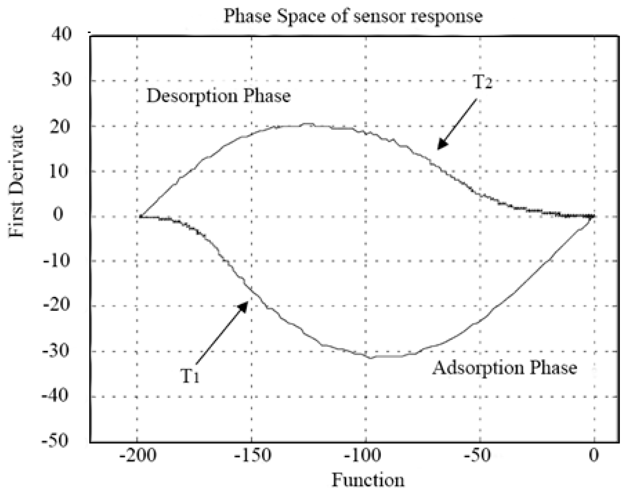
et al. described the sensor signal changes in a PS by the response values and its first derivative like
Figure 1 and then extracted the area, called phase space integral (PSI), spanned by the trajectory during the evolution either in adsorption or in desorption phase as feature, which gave a substantial improvement in terms of both error of estimation and classification [
33].
Figure 1.
Phase space of sensor with and as variables.
Figure 1.
Phase space of sensor with and as variables.
Vergara
et al. took some morphological descriptors DM in PS analogous to the second moments of the area of a geometrical figure in a 2D space into consideration. The usefulness of the method of PS and DM is assessed by analyzing the transient response of metal oxide gas sensors either to a step change in gas concentration or to thermal modulation [
71].
In [
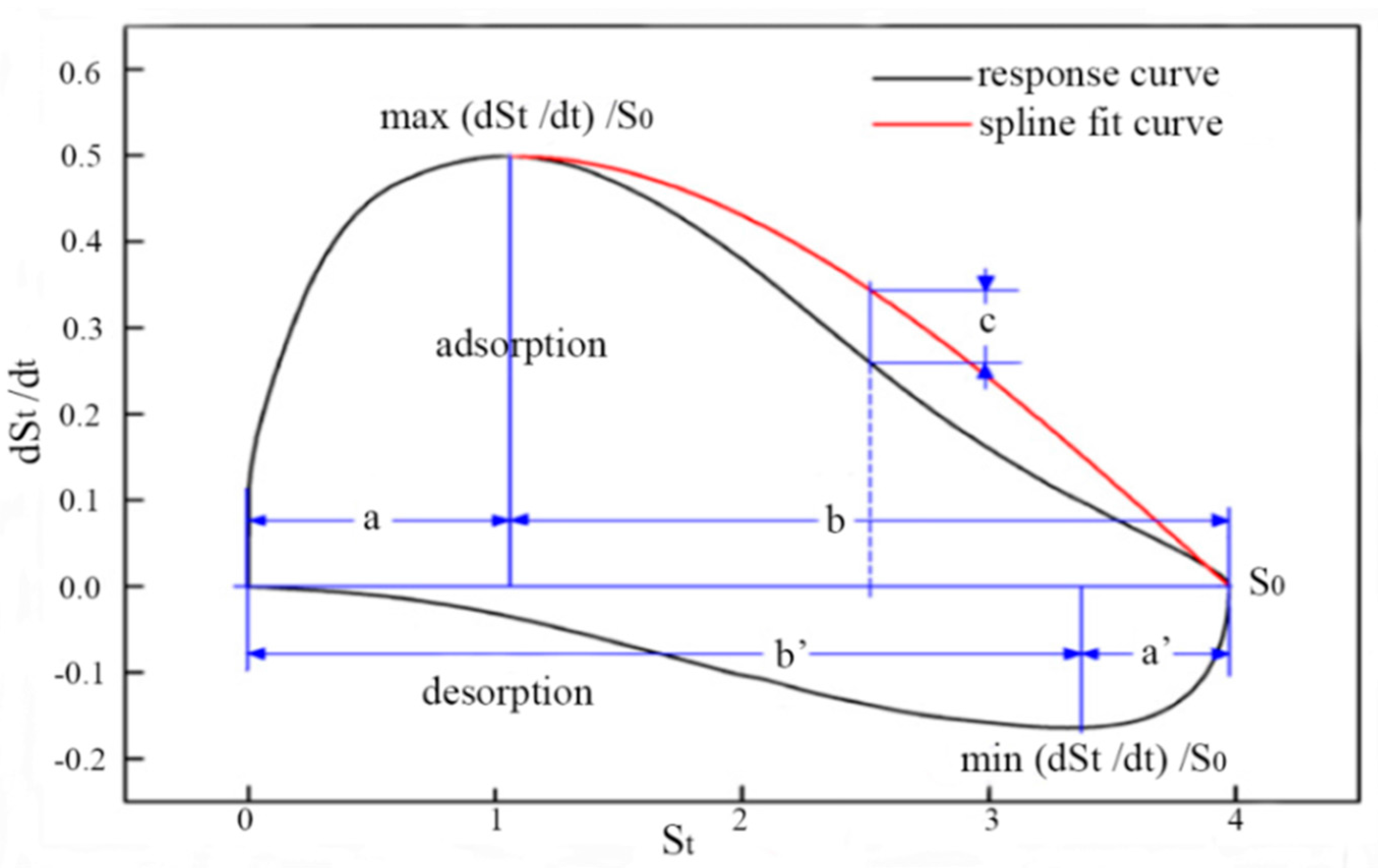
74], a gas sensor array with six TGS sensors, which were TGS813, TGS2600, TGS2602, TGS2610, TGS2611 and TGS2620, was used in the investigation on 11 kinds of gases at four different concentrations. The test gases were benzene, toluene, xylene, acetone, butanone, methanol, ethanol, formaldehyde, acetaldehyde, pentane and cyclohexane, while the four concentrations were 100, 200, 300 and 400 ppm. The phase space entire (PSE) feature extraction method extracted six features from PS (
Figure 2), which can describe the response curves completely. Suppose
to be the response of sensors, which is a function of time. Six parameters which can be obtained from the response curve in PS are
(the maximum of
), max
(the ratio of height and length in adsorption process),
(the location of ma
), min
(the ratio of height and length in desorption process),
(the location of min
) and
c is wrap value, which details are expressed in [
74]. The difference of PSE from other methods based on PS is that the sensor response curves could be reconstructed well with the six features in PSE. PSE was compared with the PSI and maximum value methods and the recognition results of three feature methods with FDA are shown in
Table 12.
Figure 2.
Six parameters extracted from PS.
Figure 2.
Six parameters extracted from PS.
Table 12.
Classification rates (CR) of different features in [
74].
Table 12.
Classification rates (CR) of different features in [74].
| Features | Number of Features | CR (%) |
|---|
| Relative difference maximum | 1 | 90.9 |
| Phase space integral (PSI) | 1 | 81.1 |
| Phase space entire (PSE) | 6 | 100 |
2.5. Other Methods for Feature Extraction
Besides the above feature extraction methods, many new original methods have been proposed in recent years. The “fingerprint” obtained from an E-nose is strongly dependent on the kind and concentration of volatiles to which it are exposed, the duration of this exposure and the temperature and humidity of the system. In some cases, it can be appropriate to increase the amount of data in order to capture as much information as possible which properly describes the system, if more reliable models are desired.
A novel method of feature extraction is the use of the three-way structure of the signals obtained from the recording of the different sensor values during a period of time, for each sample. Following this strategy, the contribution of the inner relationship between the three ways can be exploited to obtain more robust information about the system. Parallel factor analysis (PARAFAC) is one of the most popular multi-way data decomposition methods. Originated from psychometrics [
75,
76], PARAFAC is gaining interest because it is a processing technique which simultaneously determines the pure contributions to the dataset, optimizing each factor as a time, in trilinear systems. In [
35], the use of PARAFAC as a feature extraction technique from a specific three-way dataset (samples × sensors × time) for food investigation by E-noses was researched. PARAFAC performed a suitable feature extraction task, incorporating the most of the information of this complex data system. The methodology of PARAFAC also was applied in feature extraction of gas sensor data of monitoring the indoor air pollutants. The results showed that PARAFAC could more accurately monitor and predict the indoor air quality variations than multiway principal component analysis (MPCA), since it is able to capture both the time-correlations and the variable-correlation between indoor air pollutants [
36].
Due to the fact that the sensitivities of the gas sensors are different and the signals of the measured samples also are different, the energy characteristics of the signals can be used for feature extraction. An approach called global feature extraction, which focuses on the whole sensors array instead of individual sensors, based on the mutual energy of sensor signal called energy vector (EV) was introduced by Vergara [
37]. It is very useful to study the behavior of individual sensors and the theory of signals about the mutual energy is suitable to study the relations between signals of sensors belonging to the same array. The sensors of an array simultaneously interact with the same chemical pattern and as a consequence the sensor signals share a certain degree of correlation. The amount of correlation may change according to the quality and quantity of the materials to which the array is exposed. The EV was defined as:
where
was the mutual energy between signals
x(
t) and
y(
t) in the interval (
t0,
t1) and
n is the number of sensors that compose the array. The method was assessed by solving a practical problem of identification and prediction of pollutant species by building and validating a linear discriminant analysis classifier method performed by partial least squares (PLS-DA). Different validation techniques have been implemented, which have shown that the EV provides sufficient accuracy, and then it is of interest for simple, small size and real time gas analyzers. The results showed that this feature extraction methods based on EV outperformed the FFT method [
37].
Kish
et al. presented a new feature extraction method for E-noses based on a resistance noise power density spectrum (PDS), which demonstrates that even a single sensor can be sufficient to distinguish between many different chemical species [
38]. In this method, it is first assumed that only one sensor is used and its response is independent for each investigated gas. If the PDS of the resistance fluctuations in the sensor has K different frequency ranges, in which the dependence of the response on the concentration of the gases is different from the response in the other ranges, one can write:
where
dS(
fi) is the change of the PDS of resistance fluctuations at the
i-th characteristic frequency (or frequency range), and the
Bi,j quantities are calibration constants in the linear response. Thus, a single sensor is able to provide a set of independent equations to determine the gas composition around the sensor. If we have
P different sensors, and if we can use the same characteristic frequency ranges for all sensors, then we have:
where
dS(m)(
fi) is the change of the PDS of resistance fluctuations at the
i-th characteristic frequency range in the
m-th sensor and the number of independent equations is
.
Wang
et al. compared three E-nose features for tomato detection: kurtosis coefficient features, similitude entropy features and the energy features. The results showed that according to the separability measurement, the similitude entropy feature extraction method had its advantages in electronic nose detection [
77].
Figure 3.
Temporal representation of WTS.
Figure 3.
Temporal representation of WTS.
Gutierrez-Osuna
et al. [
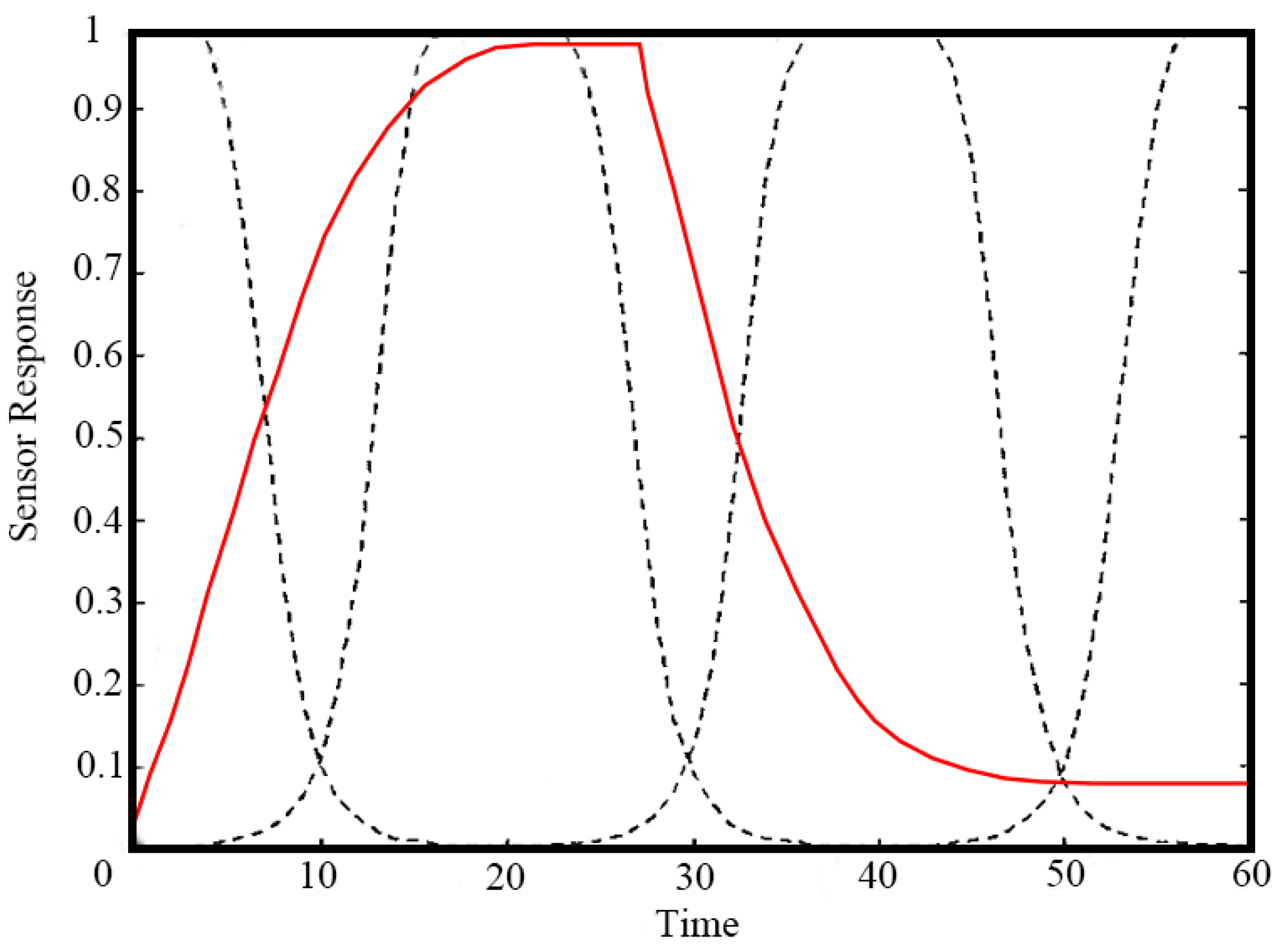
39] suggested a method called window time slicing (WTS) for creating pseudosensors based upon time slicing of sensor responses, wherein, the time response of each sensor was multiplied by four time windows to obtain the area values shown in
Figure 3. First, the response signals are multiplied by four smooth, bell-shaped windowing functions as shown in
Figure 3, and then the resulting time traces are integrated with respect to time as shown in Equation (10). In fact, the integrals are the areas surrounded by the response signal curves and the four windowing function curves. Therefore, for each sensor, four “areas” are obtained, which represent the area under the two curves. The windows are designed to overlap and span the entire response interval. These areas were further used as features and were selected using GA for classification of fragrances, hog farm air and cola beverage samples [
78]:
where
A is the feature vector extracted from one sensor which consist of four elements,
is the area surrounded by the response signal curve and the windowing function curves,
is the response value at the time
,
is the value of the
i-th windowing function at the time
,
denotes the sampling points of each curve,
is the sampling interval between two sampling points, and the parameters
define the width, shape and center of the different windowing functions
.
However, the drawback of this method is the loss of information owing to the gap between each window. In [
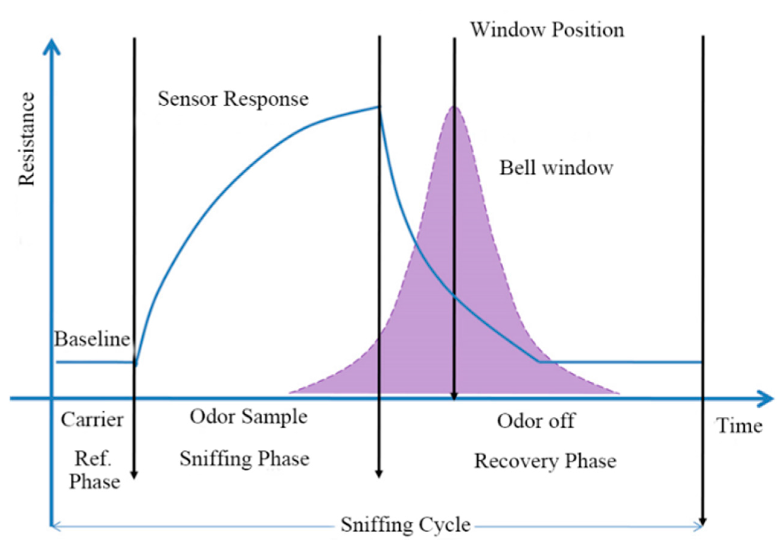
79], an attempt has been made to identify the optimum positions of the time windows in order to maximize the classification rate. To avoid the drawback of WTS, a bell shaped window defined by normal probability distribution function with mean at its position and standard deviation as 10 s was moved along the time response (shown in
Figure 4) of the sensors and simultaneously multiplied with the sensor response to obtain the area values at different positions. It can be proved that moving window time slicing (MWTS) as an approach to extract area values as features can enhance the performance of an E-nose [
80]. Comparing MWTS with other techniques
viz. peak value, rise time, fall time, DWT, FFT and WTS, it can be seen that, in
Table 13, the MWTS method performed better than the others for classification of Kangra orthodox black tea.
Table 13.
Classification rates (CR, %) of different features in [
80].
Table 13.
Classification rates (CR, %) of different features in [80].
| Features | All Sensors | Sensors 2–4 | Sensors 2 and 3 | Sensors 2 and 4 | Sensors 3 and 4 |
|---|
| Maximum value | 72.95 | 75.72 | 75.22 | 74.9 | 74.83 |
| Rise time | 75.5 | 53.43 | 41.25 | 34.95 | 36.18 |
| Fall time | 61.88 | 87.70 | 85.12 | 83.17 | 93.43 |
| DWT | 86.32 | 94.67 | 95.07 | 94.70 | 94.90 |
| FFT | 84.70 | 92.17 | 92.05 | 92.02 | 91.97 |
| WTS | 89.40 | 92.92 | 92.54 | 92.02 | 93.20 |
| SITO-WTS a | – | – | – | – | 94.52 |
| SITO-MWTS b | – | 97.35 | 96.20 | 93.30 | 96.35 |
Guo
et al. [
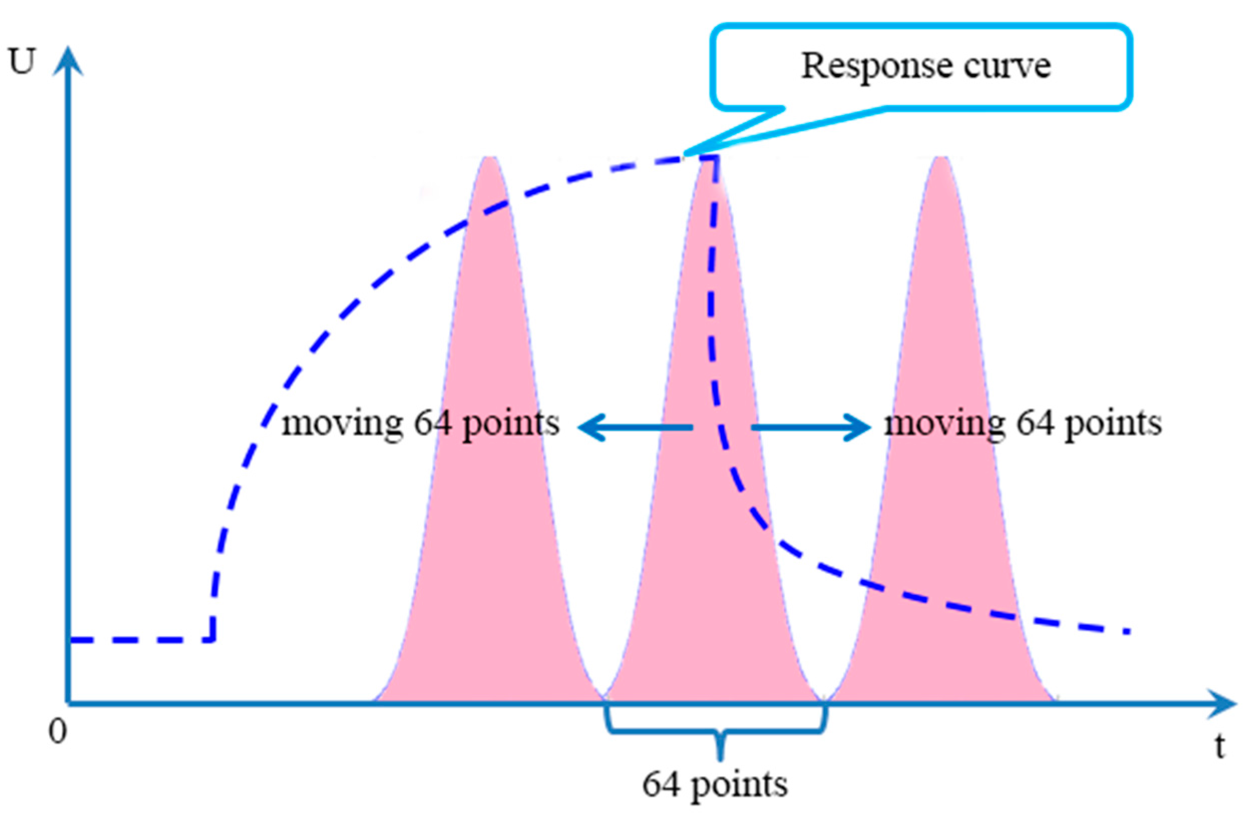
58] proposed a novel feature extraction method also based on window functions called moving window function capturing (MWFC) shown in
Figure 5. A 64 points window was placed around the peak value and then moved 64 points to the left and right along with the time axis, respectively. Thus three area values surrounded by two curves can be obtained during the moving process and the three area values were chosen as features simultaneously. The width, position, shape of the window were compared and discussed, and the final results showed that the MWFC feature performed better than the contrast features such as peak value, rising slope, descending slope, FFT, DWT and WFC, showing in
Table 14. The same conclusion can be drawn for another two E-nose datasets [
81,
82].
Figure 4.
Schematic diagram of MWTS technique.
Figure 4.
Schematic diagram of MWTS technique.
Figure 5.
The schematic diagram of MWFC.
Figure 5.
The schematic diagram of MWFC.
Table 14.
Classification rates (CR) of different features in [
58].
Table 14.
Classification rates (CR) of different features in [58].
| Feature Extraction | Accuracy Rate |
|---|
| Peak value | 87.5 |
| Rising slope | 87.5 |
| Descending slope | 85 |
| FFT | 90.0 |
| DWT | 92.5 |
| WFC | 95.0 |
| MWFC | 97.5 |


