
An Improved Inertial Frame Alignment Algorithm Based on Horizontal Alignment Information for Marine SINS

Abstract
:1. Introduction
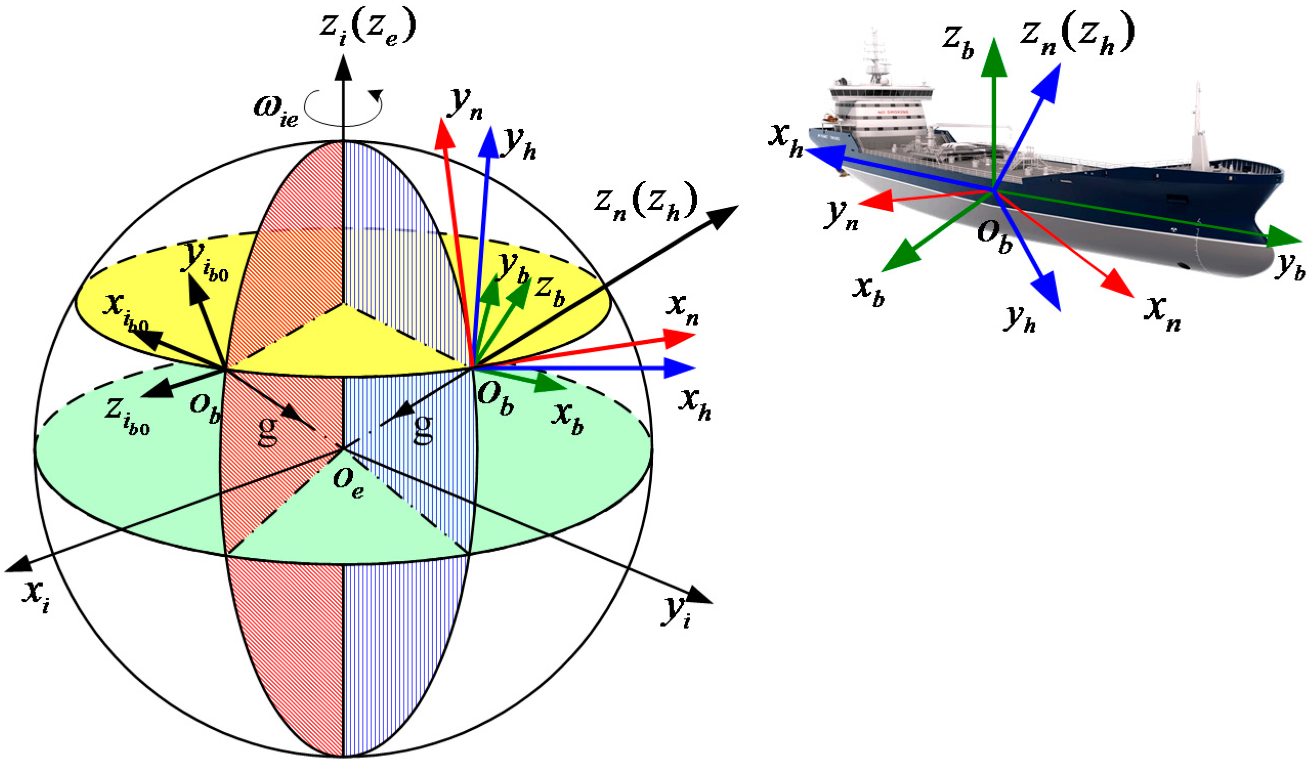
2. Reference Frames and Parameter Definitions

| Reference Frame | Definition |
|---|---|
| n-frame | Navigation reference frame which is the local horizontal reference frame. Its axes are aligned with east–north–up (ENU) geodetic axes. |
| h-frame | Horizontal reference frame. Its axis is aligned with axis, but the horizontal axes are arbitrary in the horizontal plane. |
| e-frame | Earth-centered Earth-fixed orthogonal reference frame. Its xe axis points to the local longitude. |
| b-frame | Body reference frame aligned with inertial measurement unit (IMU) axes. |
| i-frame | Earth-centered inertial fixed (ECIF) orthogonal reference frame. The axes are fixed with e-frame at the beginning of the alignment process. |
| -frame | Body inertial reference frame. It is formed by fixing the axes of b-frame in the inertial space at the beginning of the alignment process. |
| Parameter | Definition |
|---|---|
| Transform matrix from frame to frame | |
| Angular rate of Earth rotation | |
| Gravity | |
| Latitude | |
| Velocity | |
| Gyro drift | |
| Acceleration bias | |
| Misalignment angle | |
| Specific Force |
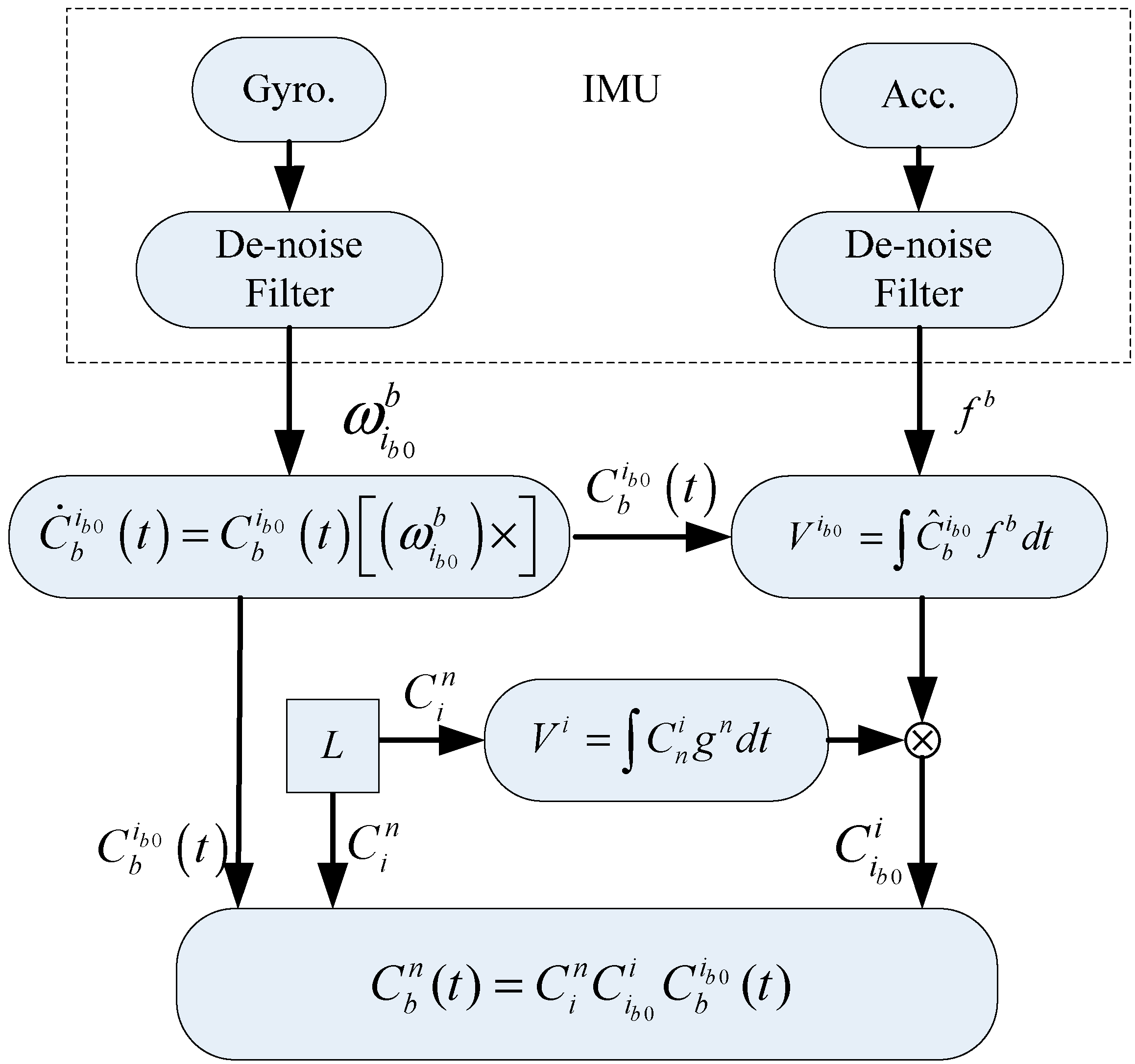
3. The Algorithmic Scheme for an Alignment Algorithm in an Inertial Frame

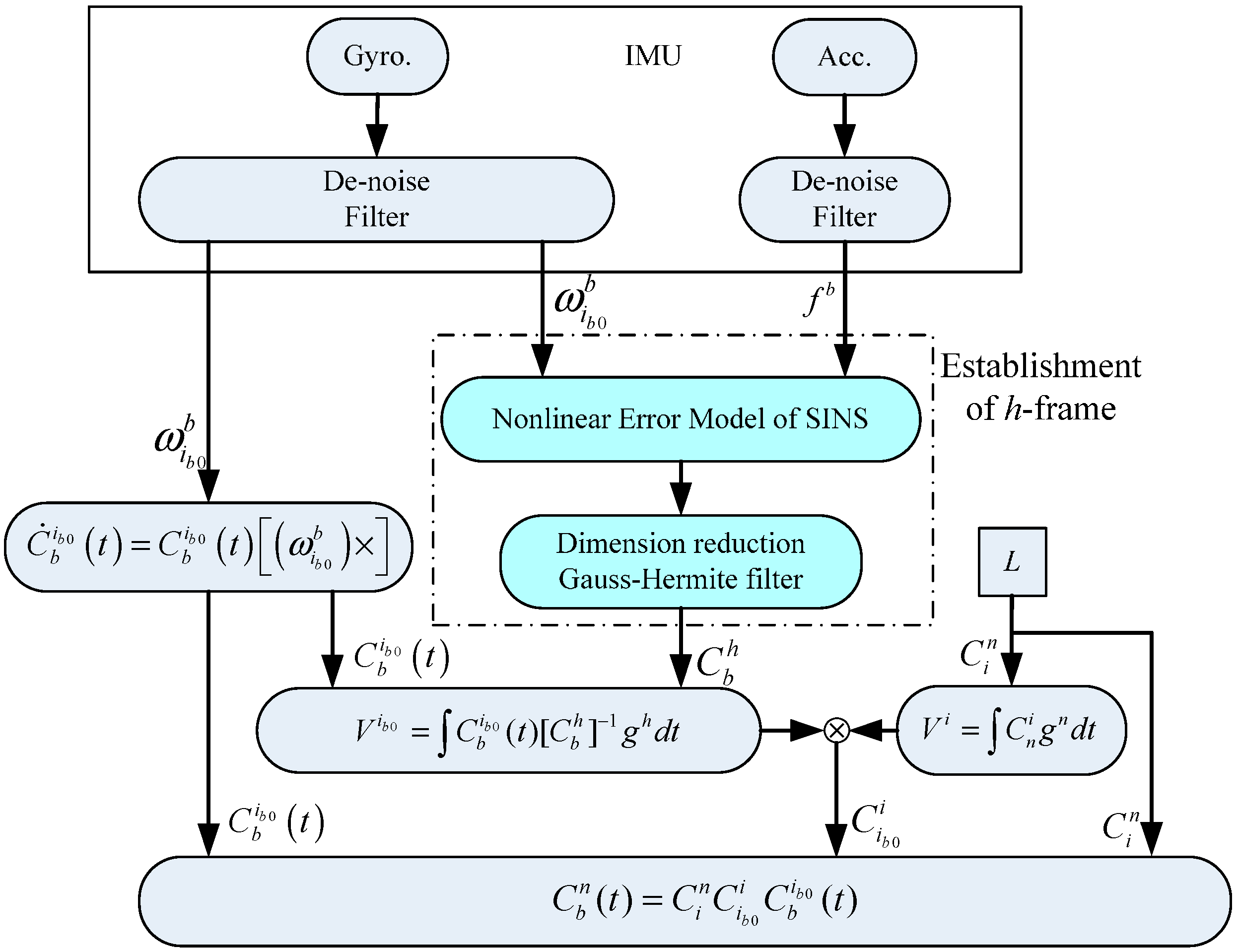
4. The Establishment of a Horizontal Reference Frame
4.1. Nonlinear Error Model of a SINS
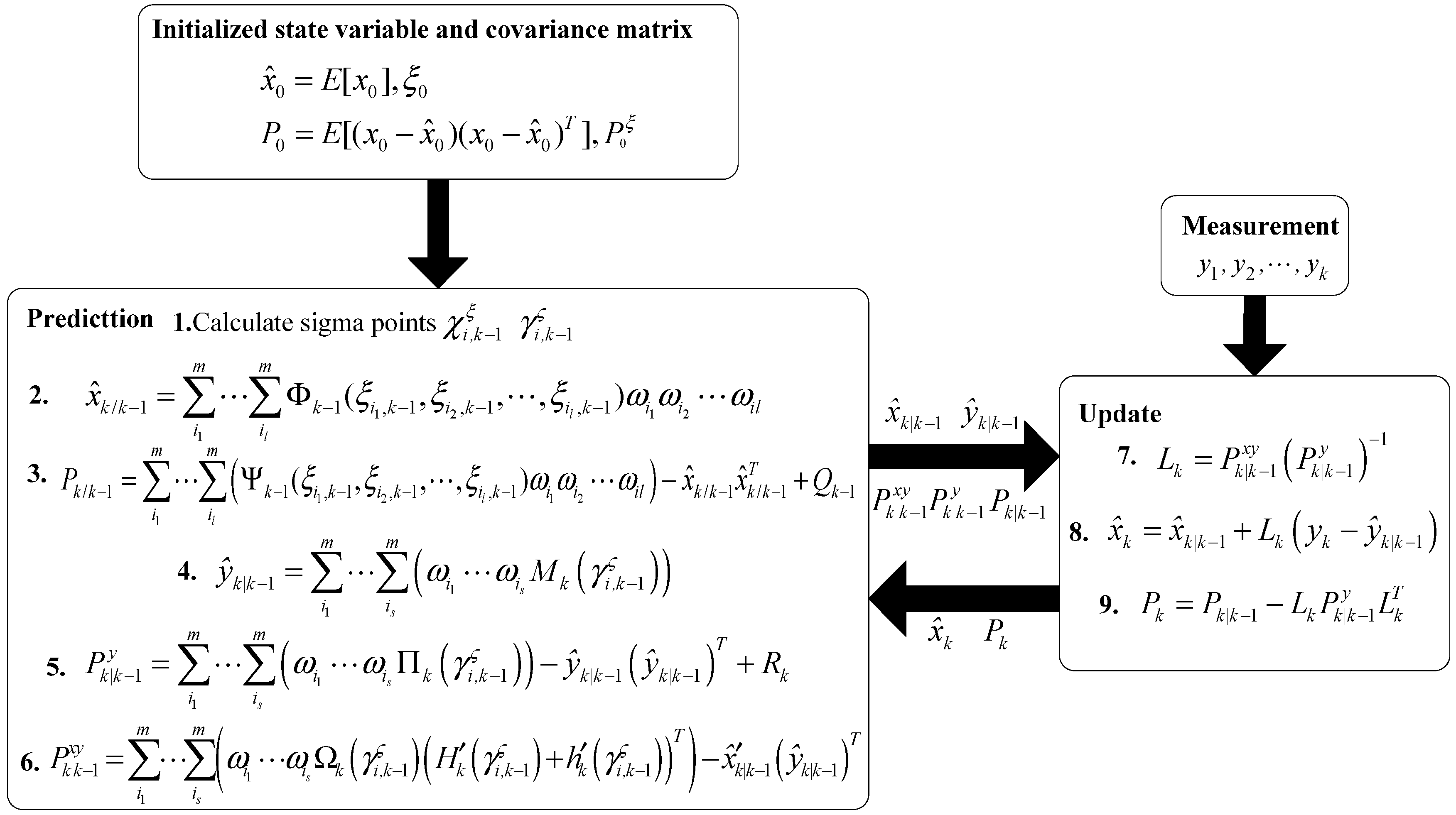
4.2. The Dimension Reduction Gauss-Hermite Filter
4.3. The Horizontal Alignment for the Large Misalignment Angle Model Based on the Dimension Reduction Gauss-Hermite Filter
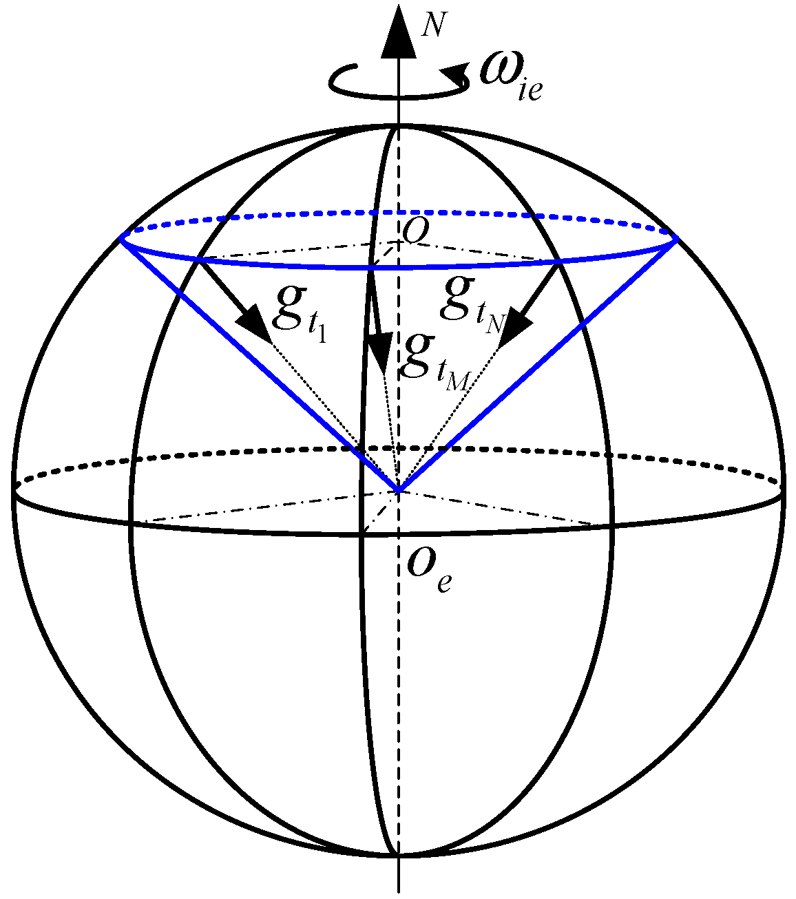
5. Calculation of the Gravity Direction
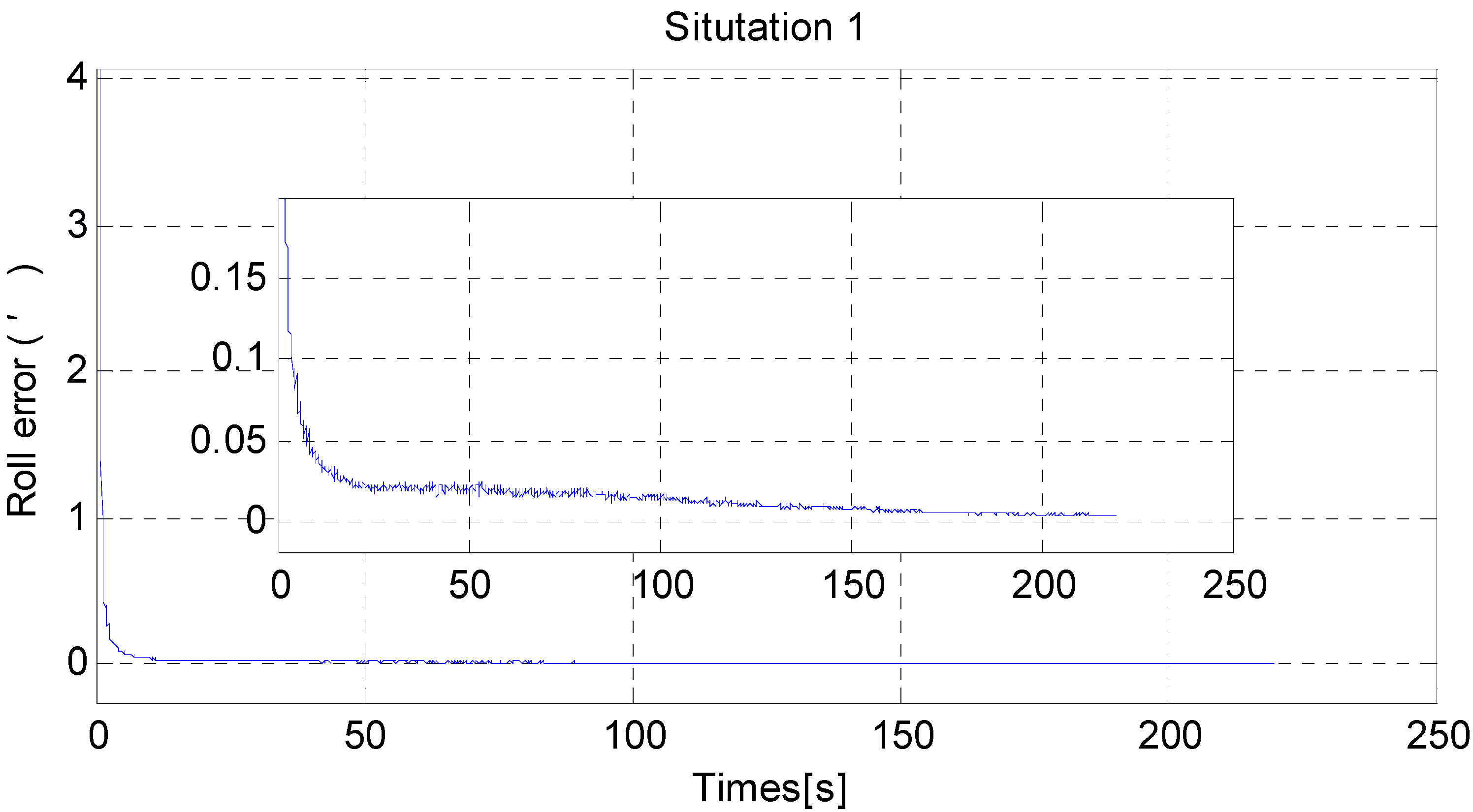
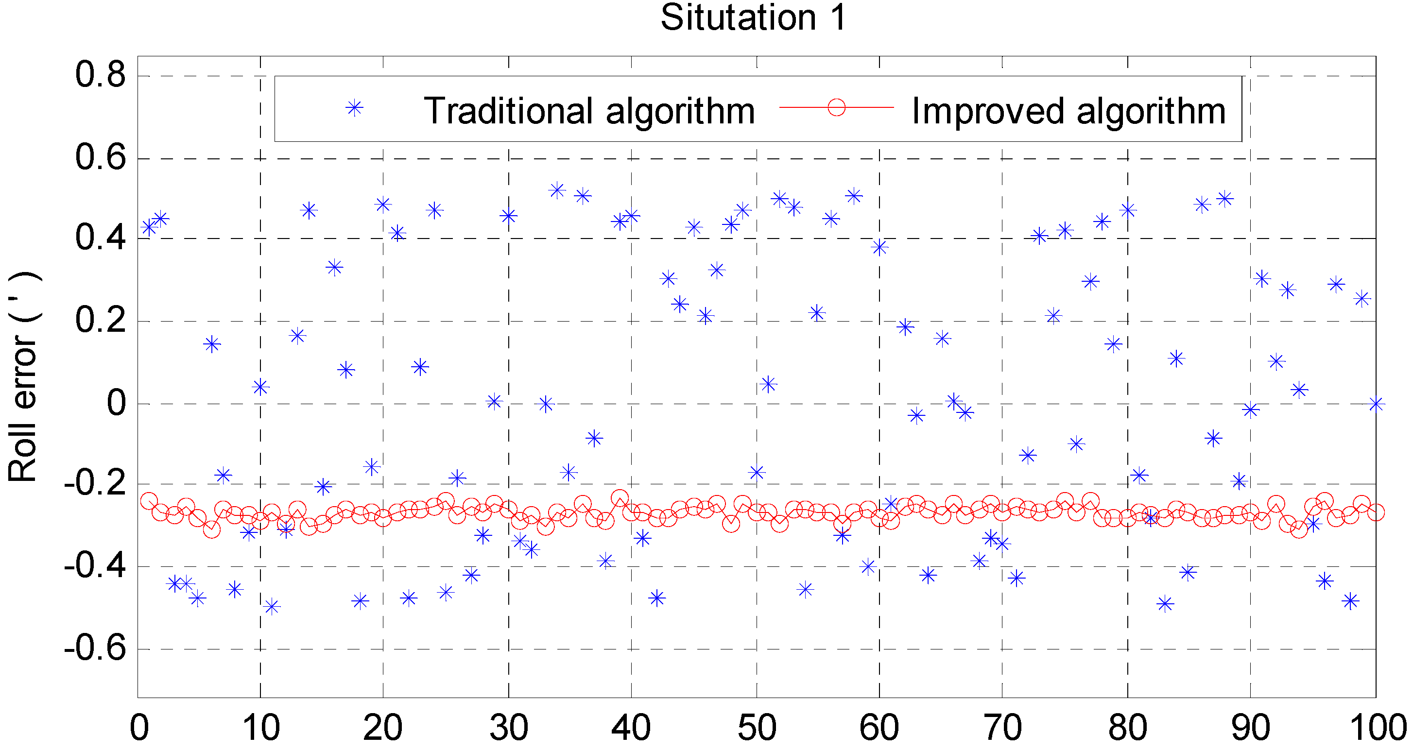
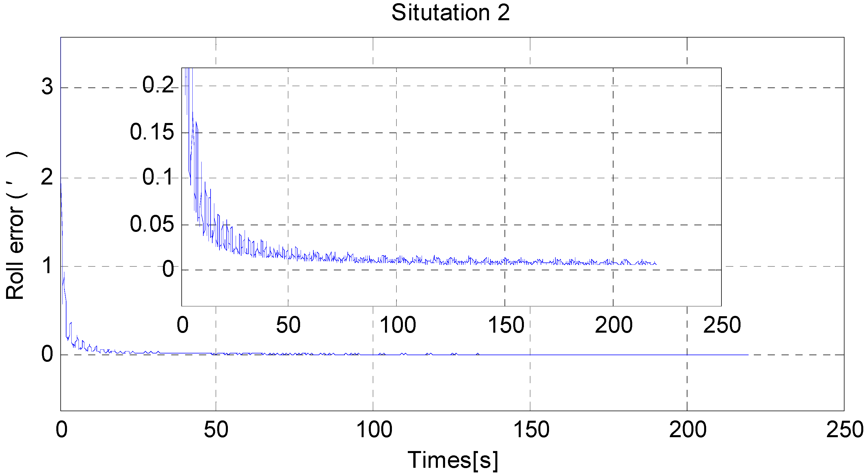
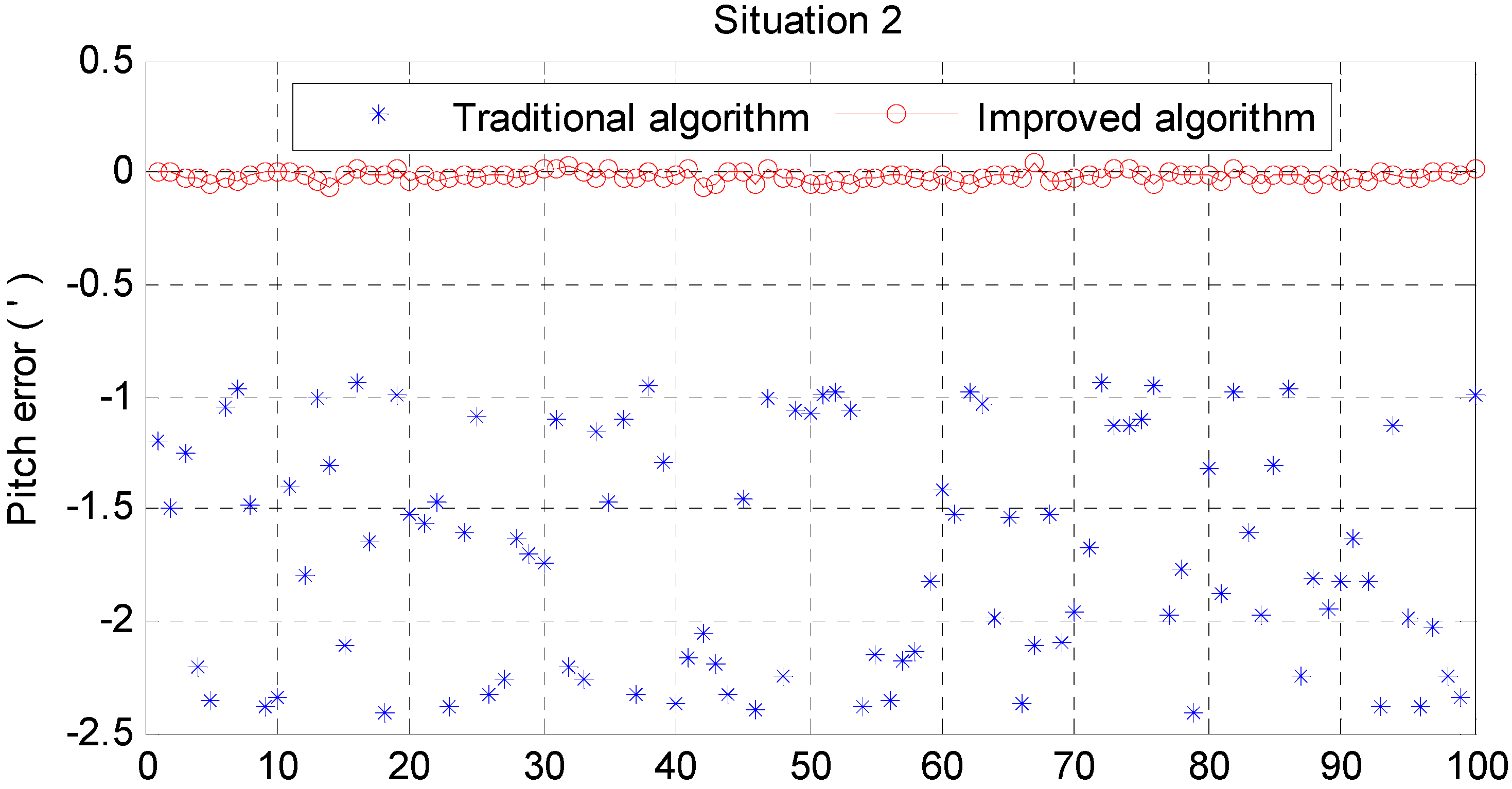
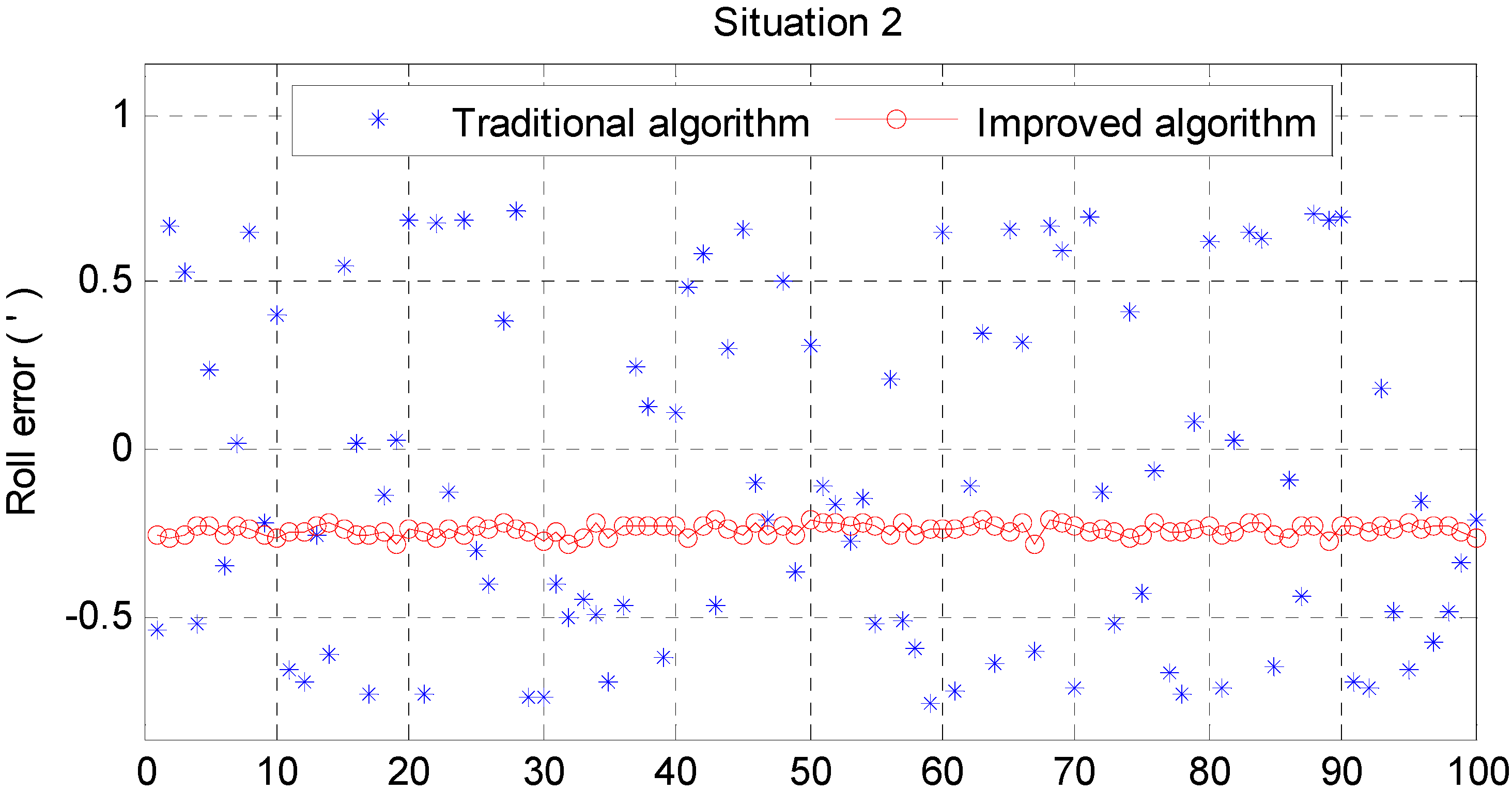
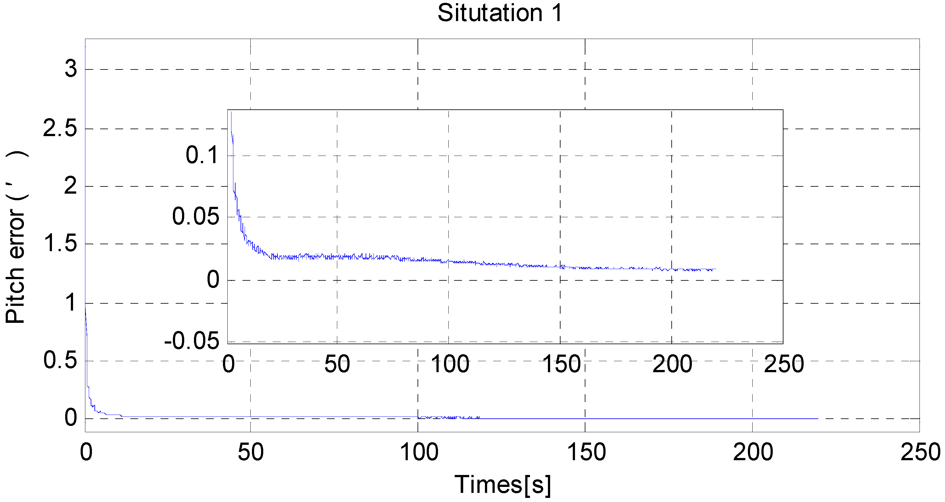
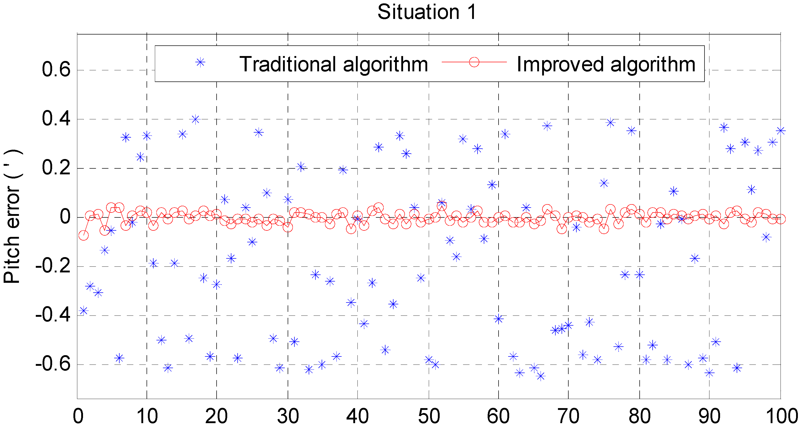
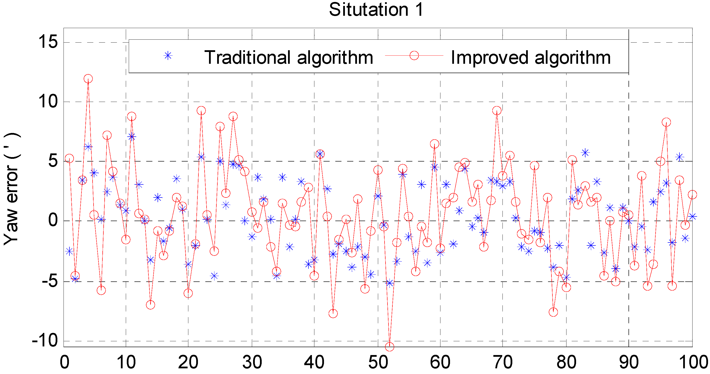
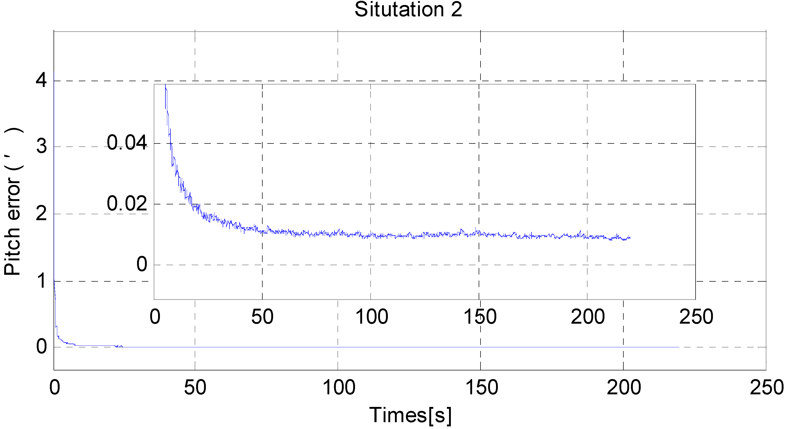
6. Simulation
| Parameters | Gyro | Accelerometer |
|---|---|---|
| Constant bias | 0.01°/h | |
| Random noise | ° |
| Traditional Algorithm (min) | Improved Algorithm (min) | |||||
|---|---|---|---|---|---|---|
| Pitch Error | Roll Error | Yaw Error | Pitch Error | Roll Error | Yaw Error | |
| Mean | −0.1677 | 0.0156 | 0.3089 | −0.0001 | −0.2679 | 0.6363 |
| Std | 0.3475 | 0.3467 | 3.0679 | 0.0231 | 0.0163 | 4.2559 |
| Max | 0.6472 | 0.5212 | 7.1117 | 0.0723 | 0.3059 | 11.9556 |


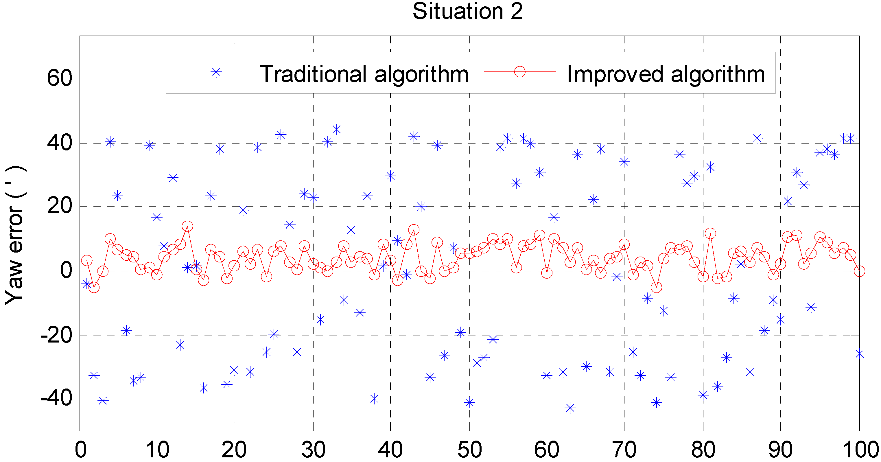
| Traditional Algorithm (angular minute) | Improved Algorithm (angular minute) | |||||
|---|---|---|---|---|---|---|
| Pitch Error | Roll Error | Yaw Error | Pitch Error | Roll Error | Yaw Error | |
| Mean | −1.6843 | −0.0872 | 2.5054 | −0.0172 | −0.2397 | 4.1585 |
| Std | 0.5111 | 0.5033 | 29.3313 | 0.02248 | 0.0174 | 4.2575 |
| Max | 2.4103 | 0.7588 | 44.1109 | 0.0680 | 0.2863 | 14.1987 |
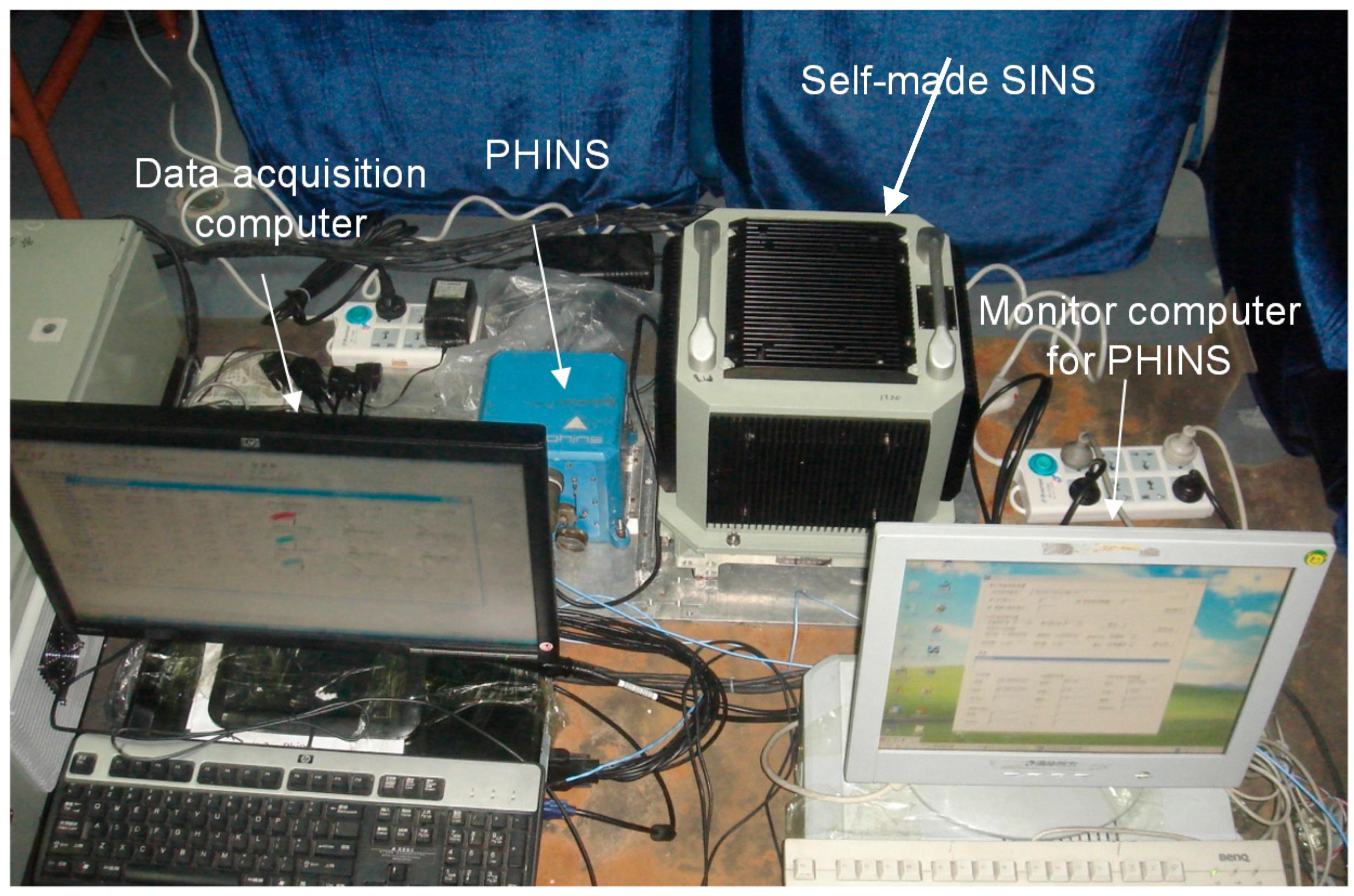
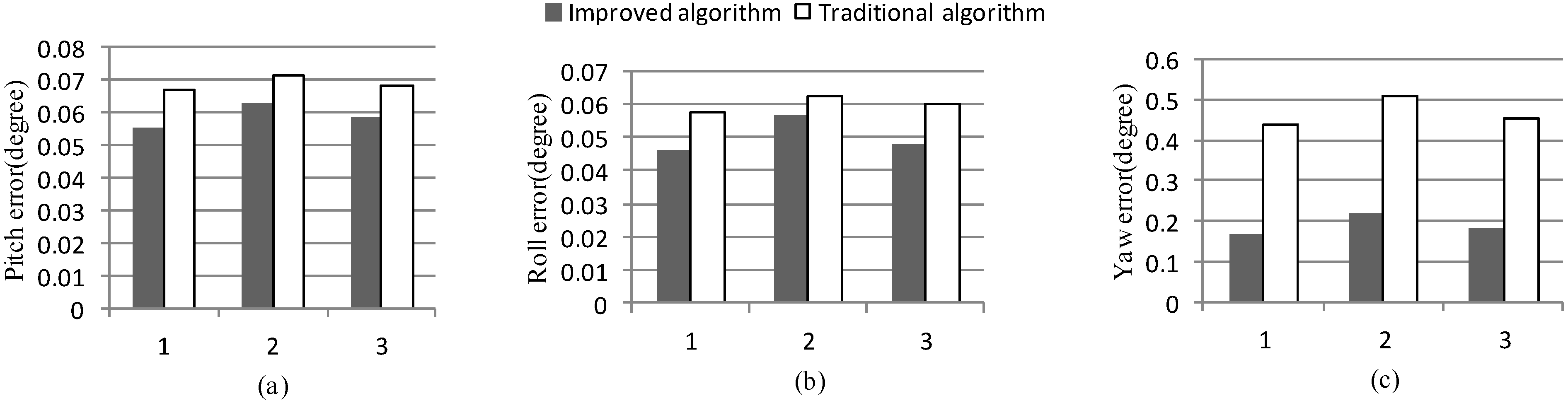
7. Experiments


8. Conclusions
Acknowledgments
Conflicts of Interest
Appendix
A. Error Analysis
B. Gaussian Approximation Filters
C. Gauss-Hermite Quadrature Point Selection
D. RMS Error
References
- Britting, K.R. Inertial Navigation Systems Analysis; Artech House Publishers: Norwood, MA, USA, 1971. [Google Scholar]
- Titterton, D.; Weston, J.L. Strapdown Inertial Navigation Technology; IET: London, UK, 2004; Volume 17. [Google Scholar]
- Qin, Y.; Yan, G.; Gu, D.; Zheng, J. Clever way of sins coarse alignment despite rocking ship. Xibei Gongye Daxue Xuebao/J. Northwest. Polytech. Univ. 2005, 23, 681–684. [Google Scholar]
- Sun, F.; Lan, H.Y.; Yu, C.Y.; El-Sheimy, N.; Zhou, G.T.; Cao, T.; Liu, H. A robust self-alignment method for ship’s strapdown INS under mooring conditions. Sensors 2013, 13, 8103–8139. [Google Scholar] [CrossRef] [PubMed]
- Gu, D.Q.; El-Sheimy, N.; Hassan, T.; Syed, Z. Coarse alignment for marine sins using gravity in the inertial frame as a reference. In Proceedings of the 2008 IEEE/ION Position, Location and Navigation Symposium, Monterey, CA, USA, 5–8 May 2008; pp. 961–965.
- Silson, P.M.G. Coarse alignment of a ship’s strapdown inertial attitude reference system using velocity loci. IEEE Trans. Instrum. Meas. 2011, 60, 1930–1941. [Google Scholar] [CrossRef]
- Sun, F.; Sun, W. Mooring alignment for marine SINS using the digital filter. Measurement 2010, 43, 1489–1494. [Google Scholar]
- Gao, W.; Ben, Y.Y.; Zhang, X.; Li, Q.; Yu, F. Rapid fine strapdown ins alignment method under marine mooring condition. IEEE Trans. Aerosp. Electron. Syst. 2011, 47, 2887–2896. [Google Scholar]
- Gao, W.; Che, Y.; Zhang, X.; Feng, J.; Zhang, B. A fast alignment algorithm based on inertial frame for marine SINS. In Proceedings of the 2012 9th IEEE International Conference on Mechatronics and Automation (ICMA 2012), Chengdu, China, 5–8 August 2012; pp. 1756–1760.
- Hong, H.S.; Lee, J.G.; Park, C.G. In-flight alignment of SDINS under large initial heading error. Trans. Soc. Instrum. Control Eng. 2002, 38, 1107–1113. [Google Scholar] [CrossRef]
- Wei, C.; Zhang, H. Sins in-flight alignment using quaternion error models. Chinese J. Aeronaut. 2001, 14, 166–170. [Google Scholar]
- Yu, M.-J.; Park, H.-W.; Jeon, C.-B. Equivalent nonlinear error models of strapdown inertial navigation system. In Proceedings of the 1997 AIAA Guidance, Navigation, and Control Conference, New Orleans, LA, USA, 11–13 August 1997; pp. 581–587.
- Dmitriyev, S.P.; Stepanov, O.A.; Shepel, S.V. Nonlinear filtering methods application in ins alignment. IEEE Trans. Aerosp. Electron. Syst. 1997, 33, 260–272. [Google Scholar] [CrossRef]
- Wang, B.; Xiao, X.; Xia, Y.Q.; Fu, M.Y. Unscented particle filtering for estimation of shipboard deformation based on inertial measurement units. Sensors 2013, 13, 15656–15672. [Google Scholar] [CrossRef] [PubMed]
- Guo, L.; Cao, S.Y.; Qi, C.T.; Gao, X.Y. Initial alignment for nonlinear inertial navigation systems with multiple disturbances based on enhanced anti-disturbance filtering. Int. J. Control. 2012, 85, 491–501. [Google Scholar]
- Kubo, Y.; Fujioka, S.; Nishiyama, M.; Sugimoto, S. Nonlinear filtering methods for the INS/GPS in-motion alignment and navigation. Int J. Innov. Comput. Inf. Control 2006, 2, 1137–1151. [Google Scholar]
- Gao, W.; Che, Y.; Yu, F.; Liu, Y. A fast inertial frame alignment algorithm based on horizontal alignment information for marine SINS. In Proceedings of the 2014 IEEE/ION Position, Location and Navigation Symposium-PLANS 2014, Monterey, CA, USA, 5–8 May 2014; pp. 1415–1419.
- Anderson, B.D.; Moore, J.B. Optimal Filtering; Dover Publications: Englewood Cliffs, NJ, USA, 1979. [Google Scholar]
- Smith, G.L.; Schmidt, S.F.; McGee, L.A. Application of Statistical Filter Theory to the Optimal Estimation of Position and Velocity on Board a Circumlunar Vehicle; National Aeronautics and Space Administration: Washington, DC, USA, 1962.
- Julier, S.J.; Uhlmann, J.K. Unscented filtering and nonlinear estimation. Proc. IEEE 2004, 92, 401–422. [Google Scholar]
- Arasaratnam, I.; Haykin, S.; Hurd, T.R. Cubature kalman filtering for continuous-discrete systems: Theory and simulations. IEEE Trans. Signal. Process. 2010, 58, 4977–4993. [Google Scholar] [CrossRef]
- Arasaratnam, I.; Haykin, S. Cubature kalman filters. IEEE Trans. Autom. Control. 2009, 54, 1254–1269. [Google Scholar] [CrossRef]
- Ito, K.; Xiong, K. Gaussian filters for nonlinear filtering problems. IEEE Trans. Autom. Control. 2000, 45, 910–927. [Google Scholar] [CrossRef]
- Gao, W.; Zhang, Y.; Wang, J.G. A strapdown interial navigation system/beidou/doppler velocity log integrated navigation algorithm based on a cubature kalman filter. Sensors 2014, 14, 1511–1527. [Google Scholar] [CrossRef] [PubMed]
- Arasaratnam, I.; Haykin, S.; Elliott, R.J. Discrete-time nonlinear filtering algorithms using gauss-hermite quadrature. Proc. IEEE 2007, 95, 953–977. [Google Scholar] [CrossRef]
- Jia, B.; Xin, M.; Cheng, Y. Sparse gauss-hermite quadrature filter for spacecraft attitude estimation. In Proceedings of the 2010 American Control Conference, Baltimore, MD, USA, 30 June–2 July 2010; pp. 2873–2878.
- Jia, B.; Xin, M.; Cheng, Y. High-degree cubature kalman filter. Automatica 2013, 49, 510–518. [Google Scholar] [CrossRef]
© 2015 by the authors; licensee MDPI, Basel, Switzerland. This article is an open access article distributed under the terms and conditions of the Creative Commons Attribution license (http://creativecommons.org/licenses/by/4.0/).
Share and Cite
Che, Y.; Wang, Q.; Gao, W.; Yu, F. An Improved Inertial Frame Alignment Algorithm Based on Horizontal Alignment Information for Marine SINS. Sensors 2015, 15, 25520-25545. https://doi.org/10.3390/s151025520
Che Y, Wang Q, Gao W, Yu F. An Improved Inertial Frame Alignment Algorithm Based on Horizontal Alignment Information for Marine SINS. Sensors. 2015; 15(10):25520-25545. https://doi.org/10.3390/s151025520
Chicago/Turabian StyleChe, Yanting, Qiuying Wang, Wei Gao, and Fei Yu. 2015. "An Improved Inertial Frame Alignment Algorithm Based on Horizontal Alignment Information for Marine SINS" Sensors 15, no. 10: 25520-25545. https://doi.org/10.3390/s151025520