Robust Curb Detection with Fusion of 3D-Lidar and Camera Data

Abstract
: Curb detection is an essential component of Autonomous Land Vehicles (ALV), especially important for safe driving in urban environments. In this paper, we propose a fusion-based curb detection method through exploiting 3D-Lidar and camera data. More specifically, we first fuse the sparse 3D-Lidar points and high-resolution camera images together to recover a dense depth image of the captured scene. Based on the recovered dense depth image, we propose a filter-based method to estimate the normal direction within the image. Then, by using the multi-scale normal patterns based on the curb's geometric property, curb point features fitting the patterns are detected in the normal image row by row. After that, we construct a Markov Chain to model the consistency of curb points which utilizes the continuous property of the curb, and thus the optimal curb path which links the curb points together can be efficiently estimated by dynamic programming. Finally, we perform post-processing operations to filter the outliers, parameterize the curbs and give the confidence scores on the detected curbs. Extensive evaluations clearly show that our proposed method can detect curbs with strong robustness at real-time speed for both static and dynamic scenes.1. Introduction
Curb detection is a crucial component in both Autonomous Land Vehicles (ALV) and Advanced Driver Assistance Systems (ADAS). Robust curb detection in real environments can undoubtedly improve driving safety and benefit those systems in various tasks. In urban environments, curbs limit the driving area. They even have the same value as obstacles, for vehicles should not drive across the curbs. Curbs can also support map building and vehicle localization [1], with their continuous and static properties relative to the scenes.
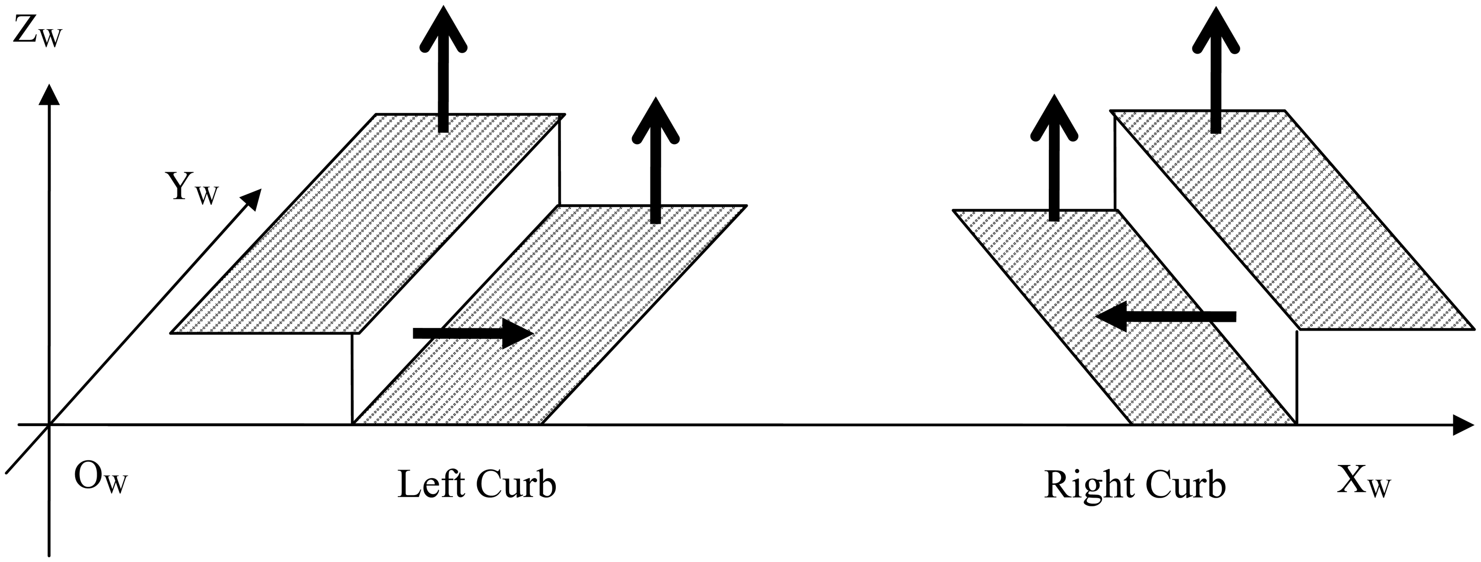
Curbs are continuous objects in the road scene and thus they have specific geometric and visual properties which serve as the backbone for robust curb detection. Traditionally, these properties are captured separately by different sensors. More specifically, range sensors measure the geometric property, while visual sensors capture the visual appearance property. We now introduce the properties of curbs in details and then explain how to better use these properties in our method to detect the curbs. From the geometric model shown in Figure 1, we can observe following critical geometric properties of curbs:
Height property. There is a height variation over curbs, and the variation range is from 5 to 35 cm.
Normal property. The normal directions change sharply near curbs. More specifically, the normal directions around the left curb are ‘up-right-up’, while the ones around the right are ‘up-left-up’.
Consistency property. The above two properties are consistent and continuous along the curbs.
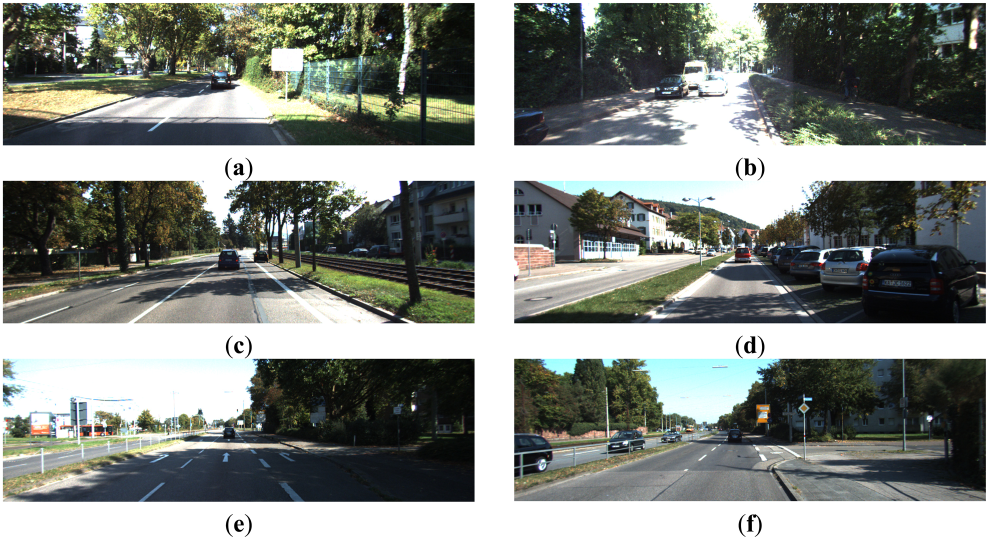
From the road images containing curbs, as shown in Figure 2, we can observe the following visual properties of curbs:
Edge property. Some curbs have visible edges in the visual image;
Variety property. There is no universal appearance model of curbs applying for different scenes.
Though curbs have the aforementioned specific properties, curb detection in various environments remains a challenging problem, even with state-of-the-art sensors. The major difficulty lies in that the curbs only have a subtle variation of height, compared with obstacles. Such subtle range changes are easily confused with noises and are hardly detected by range sensors. On the other hand, for visual sensors, edges of the curbs are prone to being confused with other objects. Such cases will be worse in cluttered scenes.
Thus, range-visual fusion seems to be a promising approach for robust curb detection. Traditional range-visual fusion methods [2,3] used the detection results from range data to guide the curb searching in the visual image, which have the advantage of enlarging the detection range. However, curb searching in visual images may be unreliable in cluttered scenes, due to the visual properties mentioned above. Therefore, in this work, we propose an alternative approach to more effectively fuse the range and visual data to enhance the robustness of curb detection. In particular, we base our approach on the state-of-the-art range-visual fusion algorithm [4], which can recover a dense depth image of the scene by propagating depth information from sparse range points to the whole high-resolution visual image. With this high-quality recovered dense depth data, our method makes full use of the aforementioned geometric properties of the curbs for robustly detecting curbs in various conditions. Our proposed method roughly comprises following four steps.
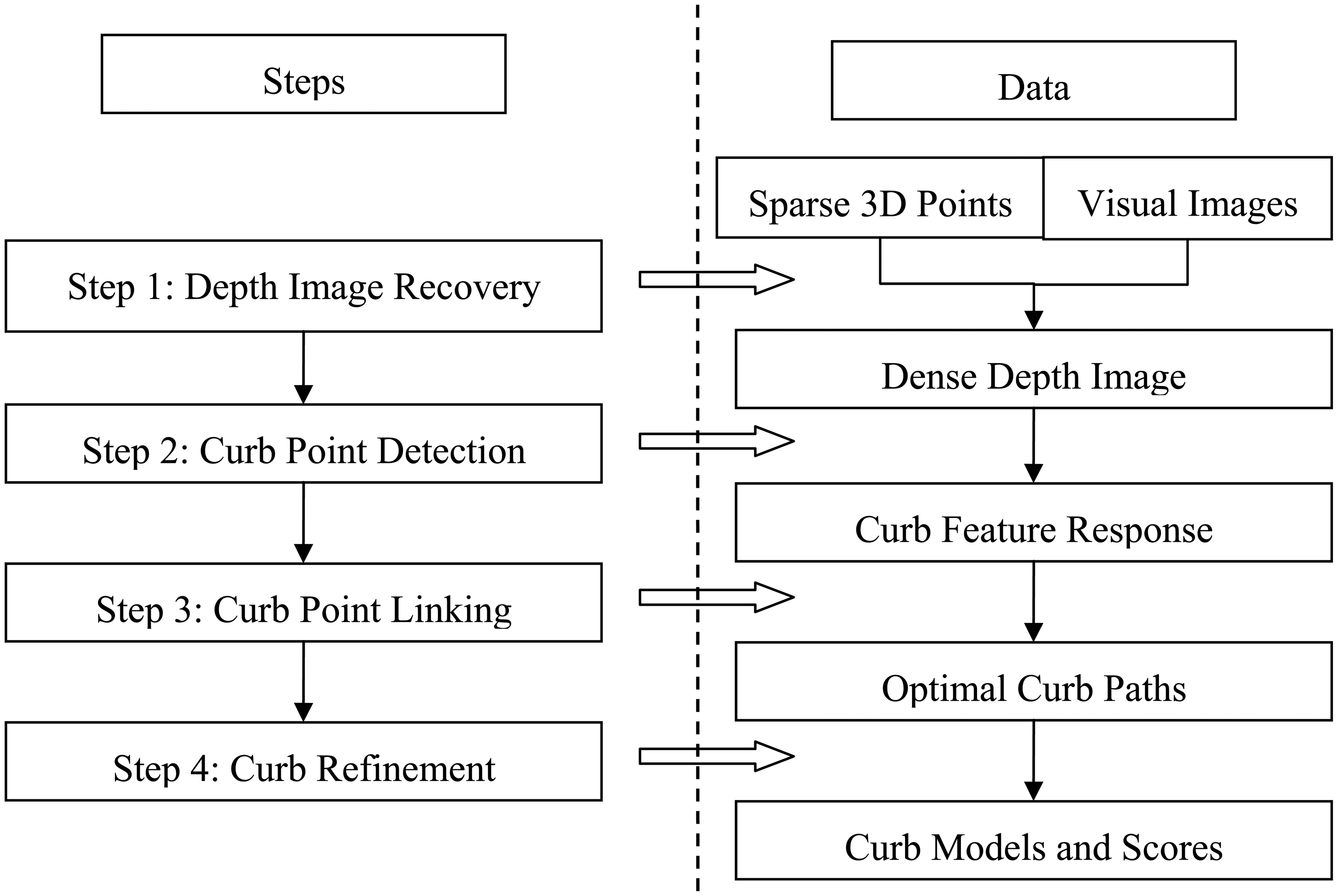
- Step 1:
Depth image recovery. Provided with the sparse Lidar points and high-resolution camera images, we recover the dense depth image of the dynamic scene based on a filter-based fusion framework [4].
- Step 2:
Curb point detection. Based on the depth image representation, we propose a filter-based method for surface normal estimation. Using the normal property, curb point features are detected in the normal image row by row.
- Step 3:
Curb point linking. As aforementioned, curbs possess the consistency property. To describe this property, we construct a Markov Chain for each road side, where each curb point is represented as a node in the chain and the connection probabilities between nodes are computed based on the consistency degree of the neighboring nodes. The optimal curb paths which link the curb points are thus found by dynamic programming.
- Step 4:
Curb refinement and parametrization. For filtering out the outliers, break points are used to cut the obtained optimal curb path into multiple segments. We choose the segment with the maximum probability as our final result, parameterize the curb by using weighted least square fitting, and compute its confidence score by considering both the node probabilities and the accuracy of the model.
A diagram illustrating the above four steps is given in Figure 3.
The major contributions of this paper can be briefly summarized as follows:
To the best of our knowledge, we are almost the first to use the dense depth image, which are obtained by effectively fusing the 3D-Lidar and camera data, for curb detection. The advantages of such data fusion for curb detection are well demonstrated in the experiments.
We propose a novel filter-based method for efficient surface normal estimation, and we show that the normal image can be used to accurately detect curb point features.
We build a Markov Chain model, using the curb point detection result, which elegantly captures the consistency property for curb point linking. The optimal curb path for each side is then linked by simple dynamic programming, which is computationally fast and cheap.
We propose several effective and feasible post-processing steps to filter out the outliers, to parameterize the curbs, and to obtain the confidence scores.
Based on the above proposed methods, we obtain robust curb detection results in various conditions (including quite bad conditions) efficiently within a long range, which is up to 30 m from the sensors. This is the best result ever achieved for curb detection to our best knowledge.
The remainder of the paper is organized as follows: in Section 2, we briefly review the existing curb detection methods with different sensors. In Section 3, we provide a detailed description of our proposed method for curb detection. In Section 4, comprehensive experiments are demonstrated in various scenes along with the quantitative and qualitative illustrations of our method. Finally, we give our conclusions and the future directions in Section 5.
2. Related Works
The research on curb detection has a long history [2], but it is still an attractive topic in intelligent robotics [5–7]. The development of these detection methods has generally followed improvements of the corresponding sensors. According to the used sensors, existing curb detection methods can mainly be categorized into: camera-based [6–13], Lidar-based [1,5,14–18], and fusion-based [2,3].
Camera-based curb detection methods have the advantage of low cost, but their performance is strongly sensitive to the outdoor conditions. For example, in low illumination, textureless, or cluttered scenes, their curb detection results may be unstable. Monocular methods utilize edge cues, and/or use texture information combined with machine learning techniques [7]. However, in curb detection, the edge cues can hardly be used as the curb edges are easy to be confused with other objects in cluttered scenes. The learning-based methods cannot apply for curb detection either. The reason is that the road and curb have great variations, and the model learned from one scene may not be suited for others. In [7], the authors tried to use Structure From Motion (SFM) to assist the information, but SFM cannot provide reliable structure estimation results under different conditions. Recently, stereo methods have become the most popular ones for curb detection [8–13]. These methods usually build the Digital Elevation Map (DEM) from the disparity, and use the edges with a certain height variation in the DEM as the cues for curb point detection. However, in textureless areas, stereo methods generally cannot provide stable range measurements, and this limits their applications.
In contrast with camera-based methods, Lidar-based methods can achieve reliable and accurate results in their valid range. However, common used Lidar sensors can only provide sparse data in a certain range, so their applicability is severely restricted in a limited area. For instance, a 2D-Lidar can only measure the distance in one scanning plane each time [5,14,15]. In order to improve the detection reliability, sequential data can be aligned with the ego-motion states [5]. At the same time, the error from ego pose estimation, which may come from abnormal shaking or relative pose drifting, will contaminate the detection result. A 3D-Lidar can give multilayer scanning data of the scene. The methods with the 3D-Lidar usually segment the ground plane first [19], and then detect the curbs in the ground surface [16,18]. For example, in [18] the authors used surface normal information, and the curbs were defined as the boundary of the plane in [17]. All those methods achieved remarkable results in their specific applications.
Fusion-based methods generally achieve better results, compared with pure camera or Lidar based methods, by integrating different information. The principle of existing fusion-based methods is to estimate reliable curbs in near region with range data at first, and then extend this result to be faraway by using the image data [2,3]. In [2], previous detection results were projected into the current image frame, and used to initialize the curb tracking in the image. In [3], the authors detected the curbs in stereo data, and used the results as the supervision signal to learn the monocular model for extended searching. The fusion-based curb tracking utilizing both 2D-lidar and camera data was proposed in [20]. There are still other sensors used for curb detection, such as the Time-of-Flight (ToF) camera [21]. However, this kind of sensor does not work at long range, or in bright sunlight.
No matter what sensors are used, all the above methods need a curb model. There are various models used in different methods, such as the straight line and line segment chain model [8], the polynomial model [9], and the polynomial spline model [10]. Generally, simple models are more robust to outliers, and sophisticated models are more accurate for describing the curb. The model parameters can be estimated by Hough Transform [8], RANdom SAmple Consensus (RANSAC) [9,18] or Weighted Least Square [2]. In [11,12] both the ground plane and curb were modeled, and in [12] past information was integrated, which can detect curbs in a range of 20 m
Other cues can also help to improve curb detection, such as the static property of the curb and the detection results of obstacles. Curbs are static relative to the road, hence, multi-frame data can be aligned to keep the persistent ones for denoising [8–10]. Explicit obstacle detection can also benefit curb detection, by removing the candidate points in obstacle region [2].
3. Fusion-Based Curb Detection Method
An overview of our method is provided in the Introduction. In this section, we introduce the details of four components of our proposed method along with the implementation details.
3.1. Depth Image Recovery
Geometric properties are important cues for curb detection. However, as mentioned, the geometric properties measured solely from the sparse range data are not robust and reliable for curb detection. In order to more effectively utilize the geometric properties of curbs, in this work, we propose to first recover a dense depth image of the scene for better curb detection, through fusing sparse range points (from the Lidar sensor) and high-resolution camera images. The dense depth image obtained in the fusion has the same resolution as the input visual images, and meanwhile has the precise depth value for each point/pixel. Thus the recovered depth image has significantly larger signal-to-noise ratio than the original range data, which is advantageous for the following curb detection. In particular, the fusion method used in this work is built on the observations that different points sharing similar features (including position, time, color, and/or texture etc.) generally have similar depth values. Fusion methods based on such assumption have shown great success in recent works [4]. Specifically, in this paper, we use the fusion algorithm proposed in [4] considering its real-time efficiency and outperforming accuracy in dynamic environments. In the implementation, the algorithm first aligns the sparse depth points with the points in the visual image frames. Then a high dimensional Gaussian filter is applied to spread the depth information from sparse points to all the image points at real time speed and generate the recovered dense depth image. For more details of the algorithm, we refer interested readers to the original paper [4].
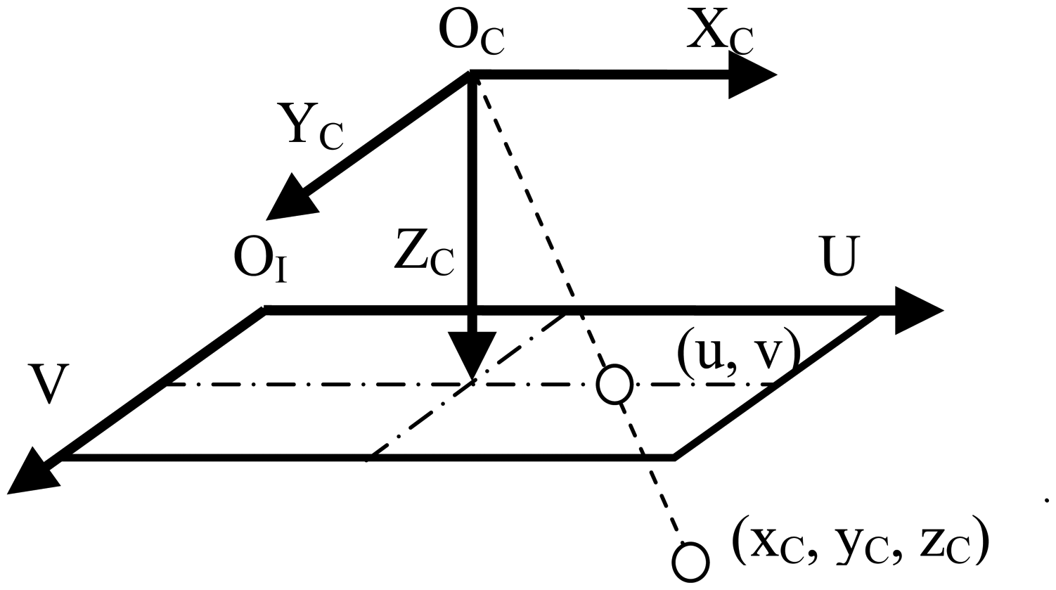
The recovered depth image is located within two coordinate systems, i.e., the image coordinate system and the camera coordinate system, as shown in Figure 4. The image coordinate system is fixed with respect to the image frame, whose origin is located at the left-top corner of the image, U-axis direction is from left to right, and V-axis direction is from top to down. Different from the image coordinate system, the camera coordinate system is fixed with respect to the camera, with its origin located at the optical center and its XC, YC, ZC–axis paralleling with U, V, optical-axis respectively. The units of image coordinates are in terms of pixels, while the units of camera coordinates are based on meters.
Figure 4 shows a depth image in these two coordinate systems. For a point having the camera coordinates (xC, yC, zC), the coordinates of its projection point in the image coordinate system (u, v) can be computed as in Equations (1) and (2) following the pinhole camera model:
In Equations (1) and (2), (fx, fy, cx, cy) are intrinsic camera parameters, which can be obtained in advance and known here. In this paper, we use the pinhole model without lens distortion to do the projection. In the cases that there is significant distortion, a distortion correction step should be conducted before the coordinate computations.
Let D denote a depth image, and d(u, v) denote the depth value of the point with image coordinates (u,v). As aforementioned, D has the same resolution as the input visual image. d(u, v) equals to the zC in Equations (1) and (2), which is obtained from the above fusion method.
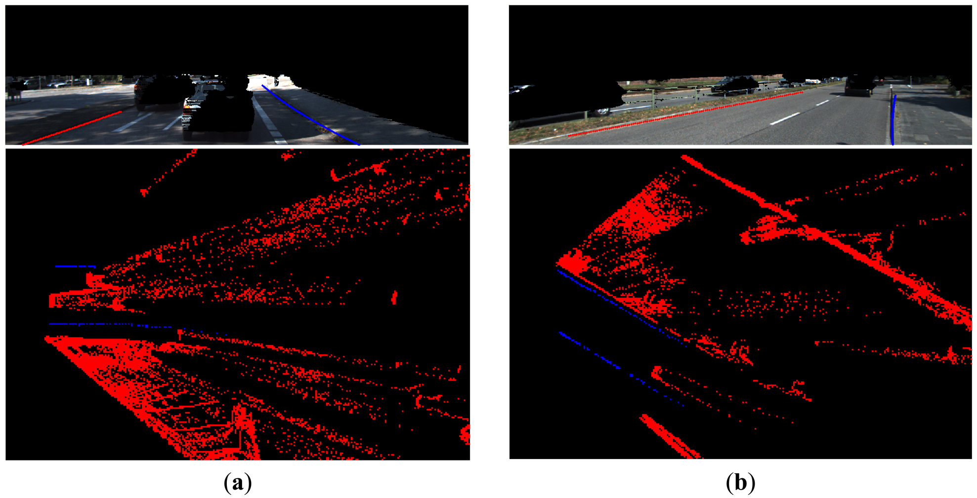
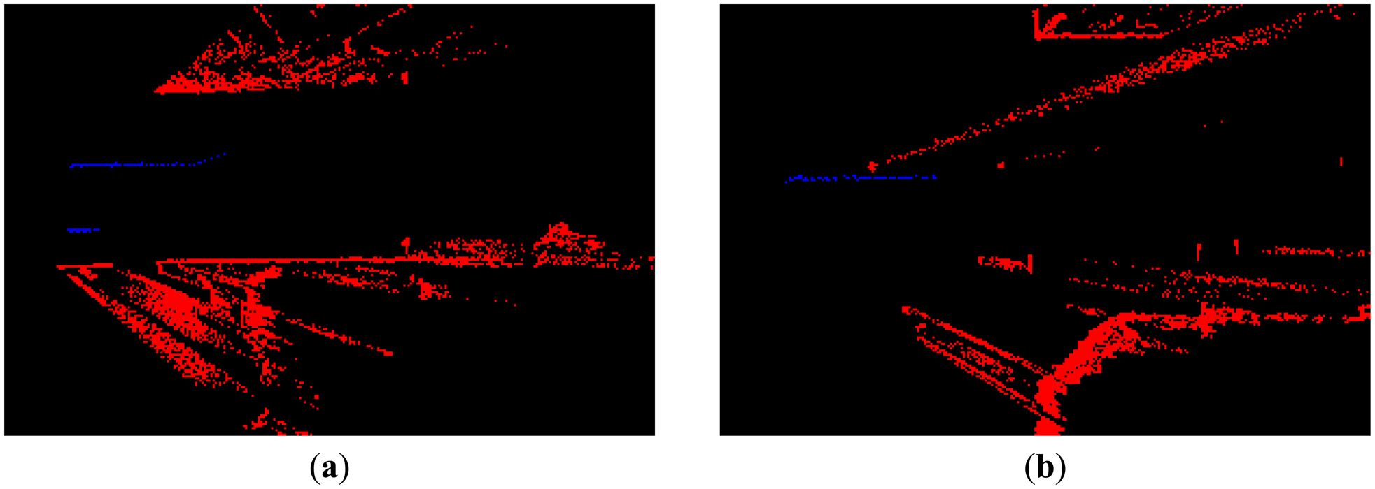
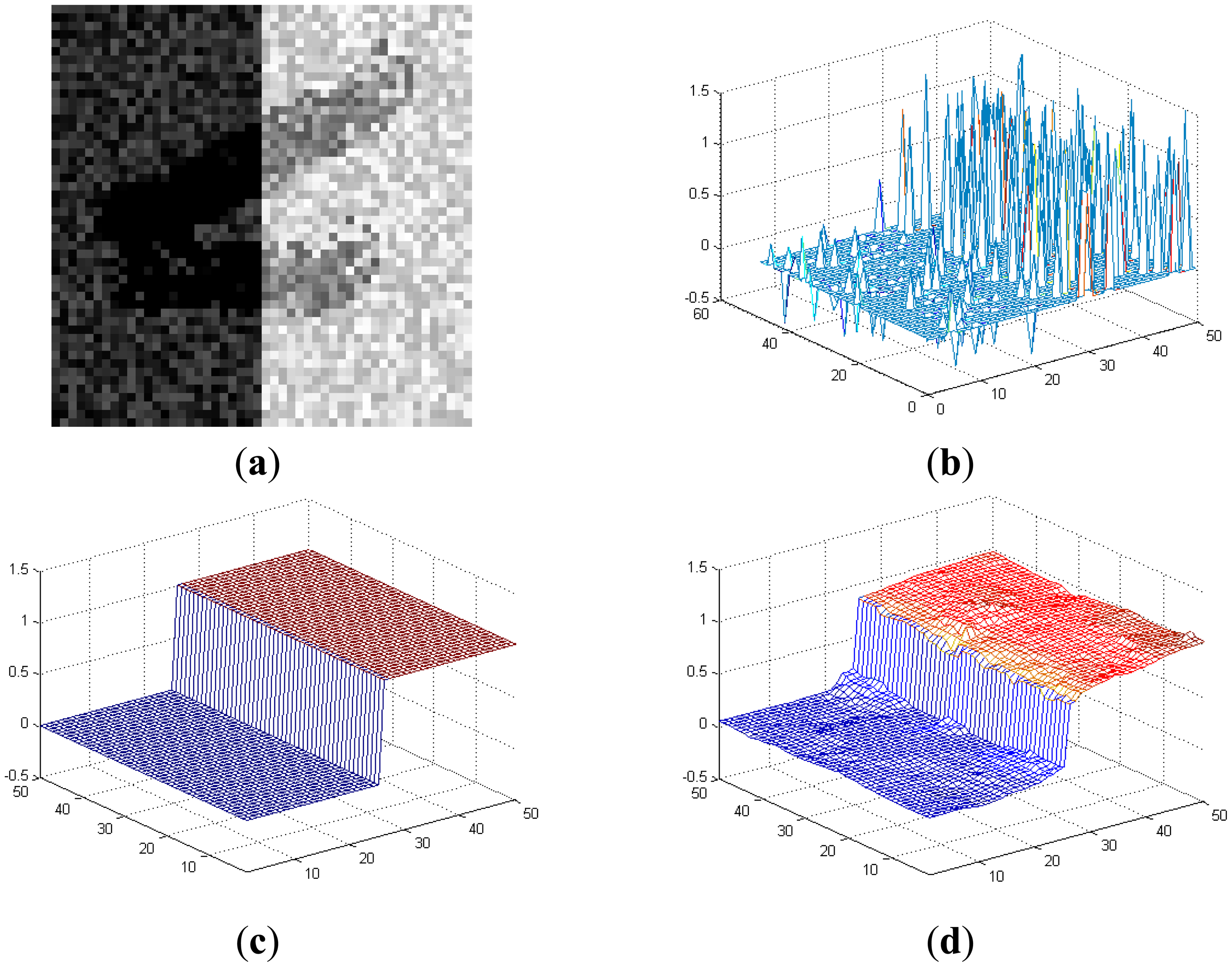
Here we provide an illustrating example in Figure 5 to demonstrate the advantages of using the depth image for curb detection. Figure 5a shows the top view of the visual image (containing random noises and shadow) of a curb segment, and Figure 5b shows the sparse range data aligned with the image. Due to the noises and shadow, we cannot accurately detect the curb on the visual or range data individually. Figure 5d shows the depth image recovered via fusing Figure 5a and Figure 5b. Obviously, recovering the dense depth image increases the resolution and meanwhile suppresses the noises/shadow of Figure 5a,b. Moreover, the curb geometric properties are clearly presented, compared with the ground truth curb shown in Figure 5c. This makes the curb detection and localization easier and more accurate.
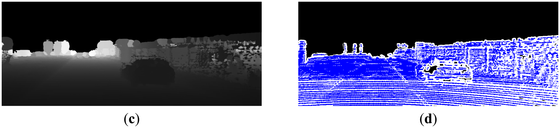
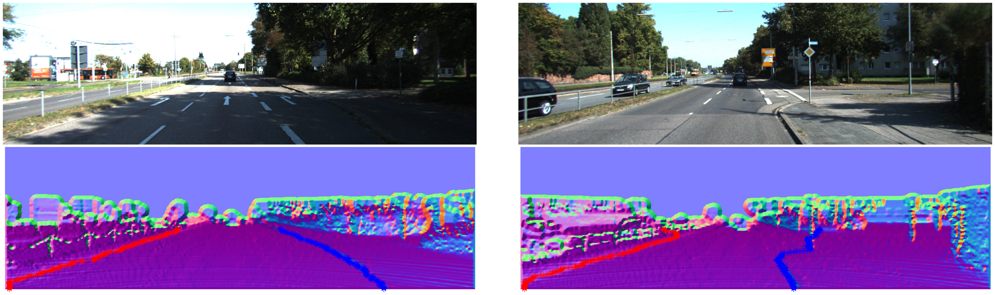
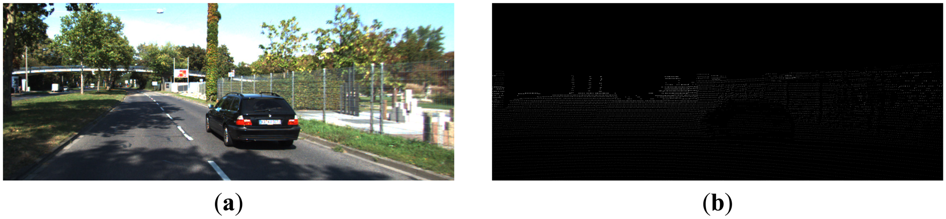
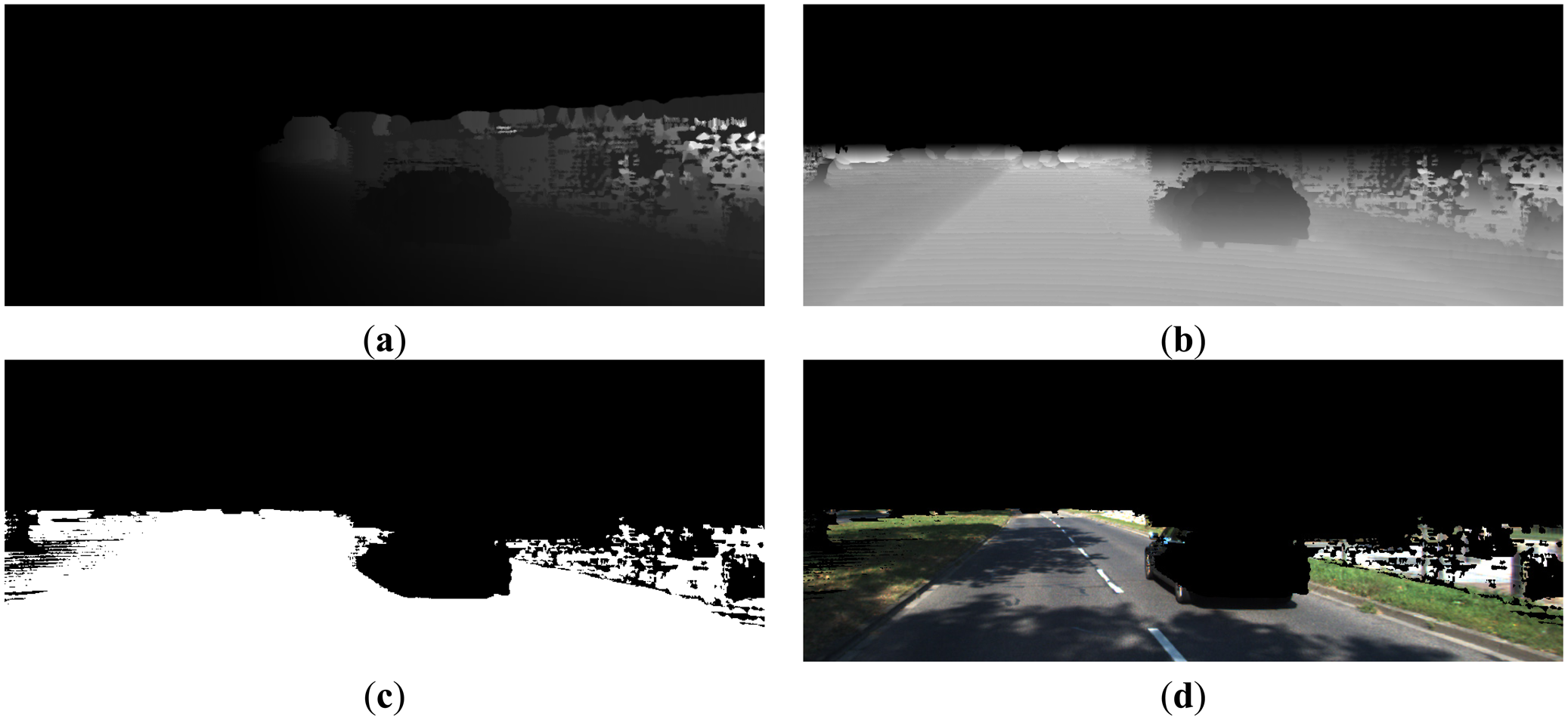
A real example of depth recovery in outdoor scenes is demonstrated in Figure 6. Similar to the above example, we obtain a dense depth image of the scene along with its confidence using the algorithm in [4]. It can be observed that depth recovery also increases the resolution and filters out the noises for the realistic scene. The confidence scores are shown in Figure 6d, in which three colors (black, white, blue) are used to distinguish different confidence levels (zero, low, high), as [4].
With the depth image, it is easy to calculate the word coordinates and camera coordinates for each point. The word coordinate system is fixed with respect to the vehicle, with its origin located at the projection point of the camera centre on the ground plane, its XW-axis pointing to the right side, YW–axis pointing to ahead, and ZW–axis pointing to the up side. The extrinsic parameters translating world coordinates to camera coordinates are the rotation matrix R and the translation vector T, which can be estimated in advance and assumed to be known here. With d(u, v) and known intrinsic parameters, we estimate the camera coordinates(xC, yC, zC) as in Equations (3), (4) and (5). The XC, YC images are shown in Figure 7a,b, respectively. Then, by applying Equation (6), world coordinates can be readily obtained with known (xC, yC, zC) and extrinsic parameters:
When zW is known, it is easy to identify the road region, whose zW < Tz. In this paper, we set TZ = 0.4 m, and the found road region and road image are shown in Figure 7c,d.
3.2. Curb Point Detection
After recovering the depth image and point coordinates in several systems, we now proceed to perform the curb point detection. First, we devise a filter-based normal estimation method using the depth image. Then, we use the curb pattern in the normal image to detect the curb point features row by row. The height property of curbs, or more precisely the fact that curbs are above the road surface from 5 to 35 cm, is also utilized for filtering out the non-road region.
3.2.1. Filter-Based Normal Estimation
In 3D information processing, surface normal direction estimation is of great importance for robotics/ALV to describe objects and understand the scenes. For unorganized 3D points, the statistics-based method is commonly used, which estimates a plane to fit each point and its neighboring points. However, this method is time-consuming for dense data. In contrast, in [22] the authors demonstrated that well organized depth data can make normal estimation fast, and they used del operator to estimate the surface normal in the spherical space. In this work, we use del operator together with the depth image representation to derive a filter-based normal estimation algorithm for dense depth images.
In particular, for one point with camera coordinates (x, y, z), its image coordinates (u, v) and depth value d(u, v) can be calculated by Equations (7), (8) and (9):
In camera coordinates, the normal estimation is formulated as del operator [22]:
With the chain rule of the derivative, the partial derivatives in Equation (10) can be expanded as:
We apply the above partial derivatives onto Equations (7), (8) and (9), and then substitute the derivative results into Equation (10), which gives:
This can be written in a compact matrix form:
In the above Equation (15), note that and are fixed for each point in the image with known intrinsic parameters (fx, fy, cx, cy); thus they can be calculated and saved beforehand to accelerate the computation. and actually compute the gradients in the u and v directions of the depth image respectively, which correspond to performing two spatial convolutions (details are given in the following), and .
For suppressing the noises, we first smooth the depth image with a Gaussian kernel (with kernel width σs) before normal estimation. Afterwards, we use the Sobel operators, defined in Equations (16) and (17), to efficiently calculate the gradient in a image convolution manner:
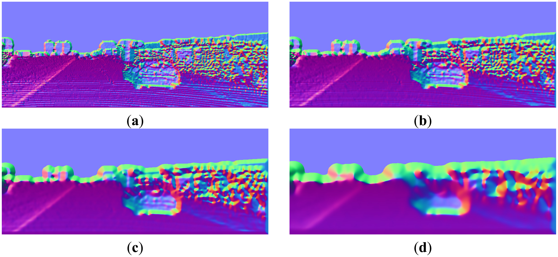
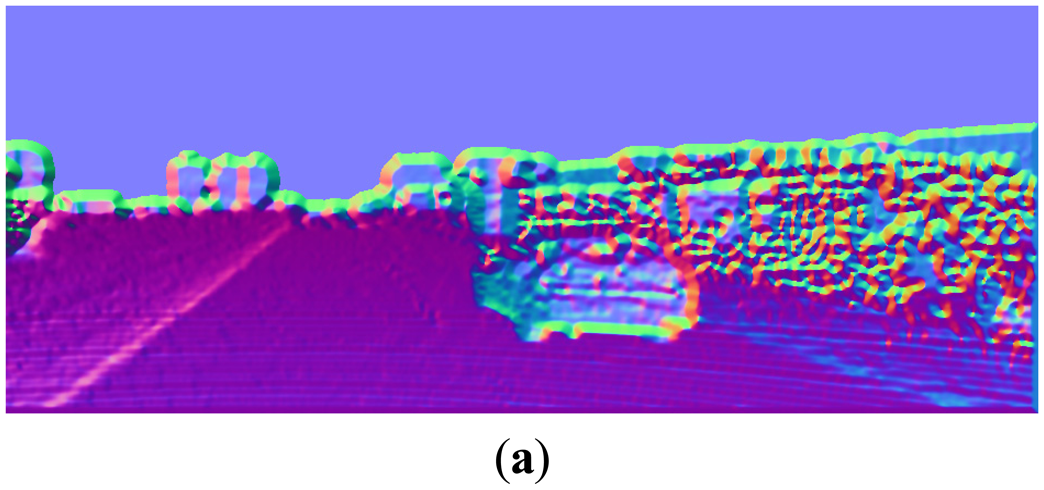
The normal estimation results, using the above convolution kernels and different smoothing kernel widths σs, are shown in Figure 8. It can be observed that, with appropriate value of σs, the convolution method gives pretty good normal estimation results. Generally the best value of σs depends on the application, which is a trade-off between reserving the details and suppressing the noises. In this paper, σs = 2 is empirically chosen throughout the experiments.
Note that this normal estimation method only needs three spatial convolutions with small kernels and some pixel-level operations, so the computation cost is quite cheap. This method can achieve accurate surface normal estimation for each point in the image. In displaying the normal direction, we use the following color codes throughout the paper. When (Nx, Ny, Nz) is the normal vector of one point, the corresponding pseudo-color used in this paper to show the normal direction is: r = (Nx + 1)/2, g = (Ny + 1)/2, b = (Nz + 1)/2, where (r,g,b) are the red, green, and blue signals respectively.
3.2.2. Curb Point Detection in the Normal Image
As in Figure 9, the normal property of curbs is clearly shown in the normal image and its projections in XW and ZW directions. In particular, in Figure 9b, both sides of the curbs appear a bright-dark-bright (BDB) pattern in row direction. Moreover, in Figure 9c, the left curb appears a dark-bright-dark (DBD) pattern, while the right curb appears a BDB pattern.
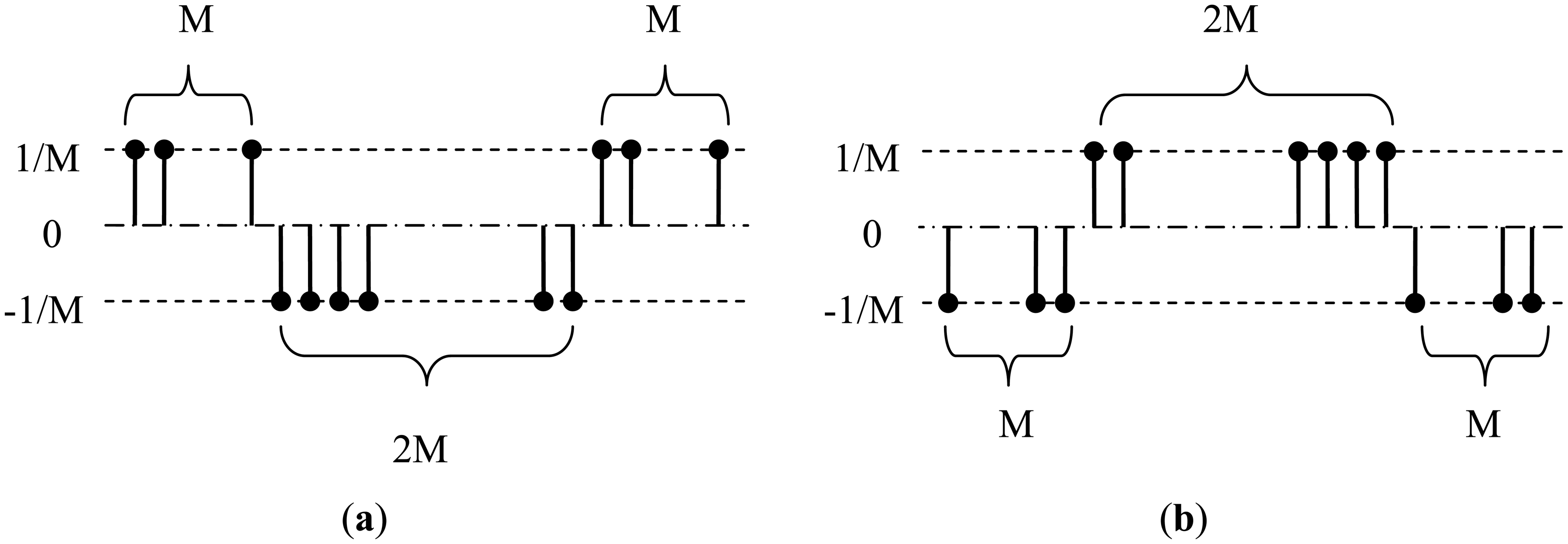
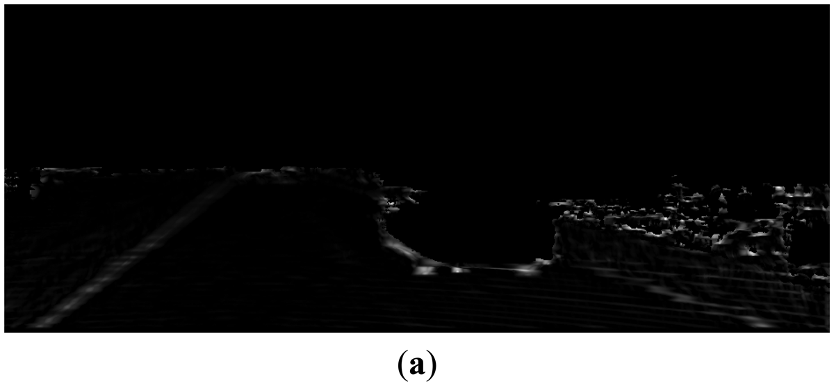
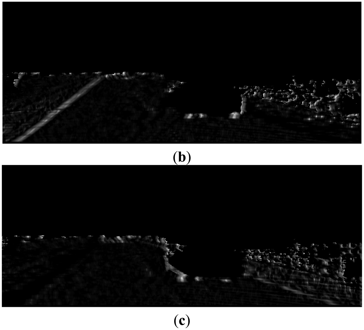
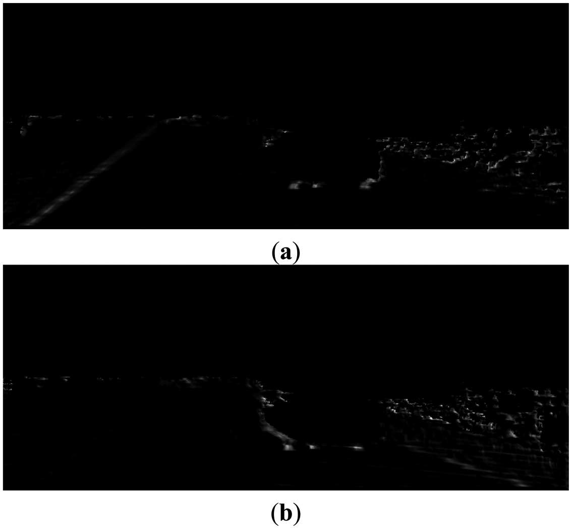
Based on above observations, we design multi-scale row patterns for better detecting curb features, which are illustrated in Figure 10. The value of M (in pixel) in Figure 10 controls the detection scale and is chosen from {1, 2, 4, 8, 16} in this paper. For each pattern, the largest response over different scales at one point is taken as its final output at this point. Some examples of the responses of the designed patterns in road region are shown in Figure 11.
We define the curb feature for each side of the curb based on the pattern responses. The left curb feature, as shown in Figure 12a, is detected by the ‘BDB’ response on the ZW projection map (Figure 11a) multiplied by the ‘DBD’ response on the XW projection map (Figure 11b). Similarly, the right curb feature, as shown in Figure 12b, is detected by the ‘BDB’ response on the ZW projection map (Figure 11a) multiplied by the ‘BDB’ response on the XW projection map (Figure 11c). As observed from the point feature detection results shown in Figure 12, the real curb positions have significant responses, although there are still some isolated noises.
3.3. Curb Point Linking
Using the consistency property of the curbs, we build a Markov Chain model for linking the curb points. After transforming the feature responses into node and edge probabilities in the Markov Chain, we can link the best curb path by high efficient dynamic programming algorithm [23,24]. This linking step at the same time filters out the isolated noises and achieves consistent curb paths.
3.3.1. Markov Chain Model for Curb Point Linking
We build a Markov Chain model for the curb in each road side, to make full use of the feature responses and explore the consistency property of the curbs.
Denote the curb point position in each row of the image as a random variable xi, and each xi has N different states, each of which corresponds to a specific column of N columns in the image. Here we restrict our model in road region, which is identified by the value zW in Section 3.1.
The node probability (i.e., the probability of xi taking a specific state from the total N states) from the curb feature is defined as:
The edge probability which describes the consistency property is defined as:
The major consideration in defining this edge probability is that the best path should be smooth in terms of both position and feature. The feature f here can be of various types, such as position, texture, color, etc. In this paper, we use the curb point feature response as f for efficiency, and we choose σf = 0.001 and σx = 10 in all our experiments.
3.3.2. Link the Curb Points via Dynamic Programming
With the node and edge probabilities defined above, the best path (linking curb points with the largest total probability) can be obtained by applying dynamic programming algorithm. The linking process includes forward and backward searching steps.
In the forward searching steps, the algorithm selects the path from top to bottom. We calculate the probability from the top row (in road region) to current point with Equation (23) and find the best link point (with the largest cumulative probability) with Equation (24):
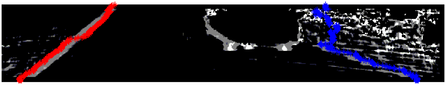
In the backward steps, we choose the point with the maximum probability in the bottom row, and track back to the top by using the link data. In this way, best paths can be linked to filter the isolated noises. The Markov Chain based curb point linking results are shown in Figure 14. We can see that the curb points are linked together accurately. On the right side, some non-curb points are also included because of the occlusion. This motivates us to propose following post-processing steps to filter out these outliers and build the curb models.
3.4. Curb Refinement
In this subsection, we introduce the details of employed post-processing in this work for further refining the curb detection results.
3.4.1. Noises Filtering
By analyzing the positions and the curb point features along the best path, we detect suitable break points to cut the best path into several segments, and choose the best segment as our final output to filter out the non-curb parts. After an average smoothing, we calculate the curvature and feature variation along the best path. Throughout the experiments, the break points are defined as points with the curvature greater than 10 or the feature variation greater than 0.003. We sum up the probabilities along each segment, and choose the segment with the largest probability as the output best segment.
3.4.2. Curb Modeling
We use a polynomial model (up to second order) in the curb modeling, which is given in Equation (25). There are also other choices for curb modeling [8–10]. We choose this polynomial one based on its simplicity and its reliability in the experiments:
We use weighted least square for estimating parameters (a,b,c) by using the nodePot as the weight for each point. For optimizing the parameters, we minimize the objective function in Equation (26):
Here (ui, vi) is a curb point in the best segment, and wi is the . With a weighted least square method, the best parameters can be estimated by solving Equation (27). The Equation (27) actually has closed form solution and can be solved fast:
3.4.3. Confidence Scoring
We give our confidence scores for the detected curbs based on both the node probability and the accuracy of the model:
That is to say, more points lying in the path with stronger curb feature and less model error can lead to a higher score for the detection result. The refined results are shown in Figure 15, where we set σsc = 3.
4. Experiment Results and Discussion
In this section, we present the experimental evaluations of our proposed method for curb detection. Here we use the widely used KITTI dataset [25] as the test bed for our curb detection method in urban environments. Based on the results in typical scenes, both qualitative and quantitative analyses of the performance of our method are given.
4.1. Dataset
We use the KITTI dataset in this section to evaluate our method. The KITTI dataset is one of the most comprehensive datasets for ALV applications, which is commonly used as the test bed for various tasks [25]. In the KITTI dataset, synchronous data from an Inertial Measurement Unit (IMU), a 3D-Lidar (Velodyne Lidar), two stereo cameras are provided at 10 Hz. The camera images are rectified, and the cameras are triggered by the 3D-Lidar to guarantee them to be well aligned. Moreover, the accurate calibration parameters for all sensors are provided.
4.2. Curb Detection Results under Various Conditions
We conduct comprehensive evaluations of our method on KITTI dataset, and our proposed method achieves outperforming results. In this section, we present some evaluation results under different conditions.
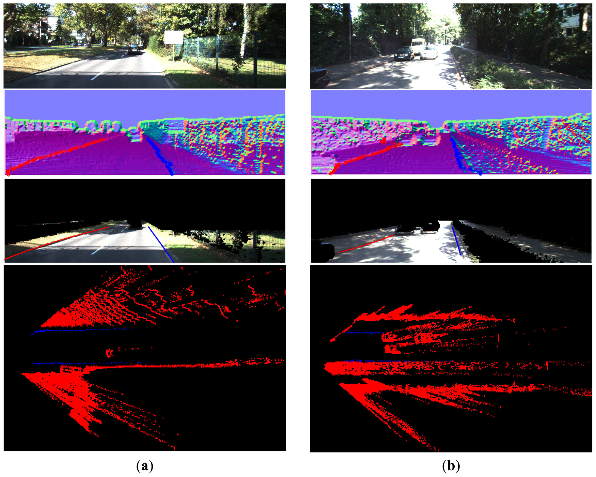
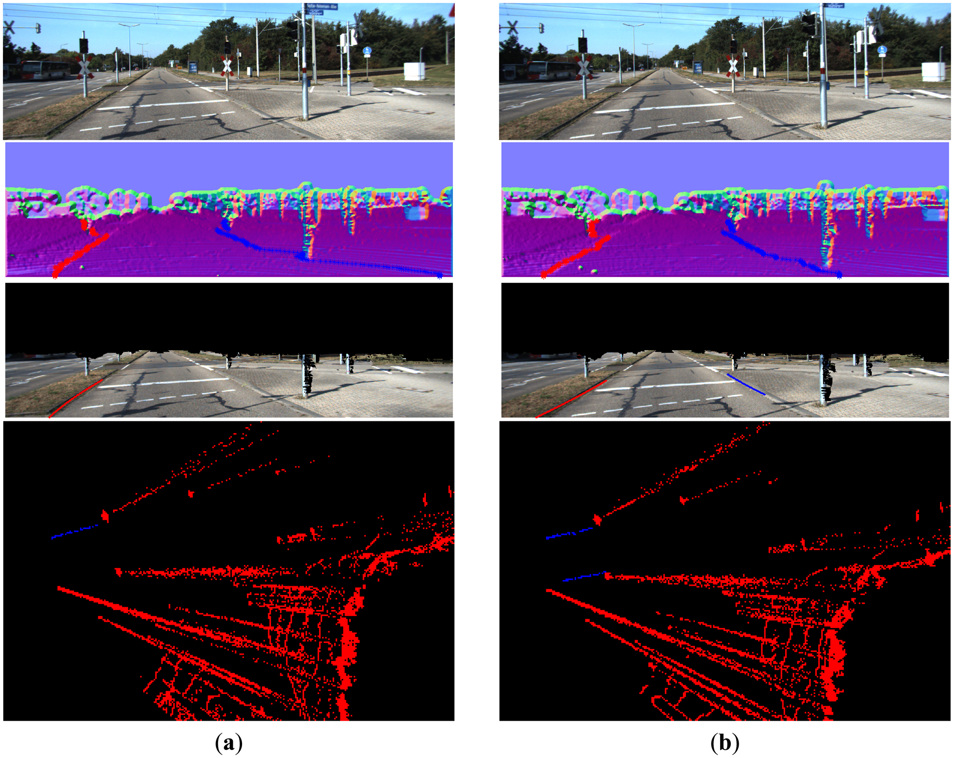
From Figures 1617, 18, 19, 20 and 21, the first row shows the visual image, the second row shows the normal image together with the best curb paths, the third row shows road image together with final curb detection results, and the last row shows the result from the top view. In the top view map, red points represent the obstacles, blue points represent the curb results, and the cover range is 60×40 m.
The statistics results of each experiment are summarized in Table 1. For each experiment, we provide the curb detection range in world coordinates and the confidence score for each side.
4.2.1. Illumination Change and Strong Shadow
Figure 16 gives the results in the scenes with illumination change and strong shadow. As can be observed from the results, our method provides results resistant to the shadow influence as it uses the geometric properties for curb detection. In Figure 16a, some curbs without corresponding edges in the image are also reliably detected.
4.2.2. Different Road Widths
Figure 17 shows the curb results with different road widths. Our method suits for both narrow and wide roads and provides satisfactory results. In Figure 17a, it is shown that our method can detect the left curb which is quite far away. The detection range in horizontal is from −8 to 8 m, and in vertical is from 6 to 30 m, as summarized in Table 1. This detection range is quite sufficient in practice.
4.2.3. Straight and Curved Curbs of Different Lengths
For detecting both curved and straight curbs of different lengths, our method provides reliable detection results, as shown in Figure 18. In Figure 18b, the right curb, which only occupies a small part of the road, is also successfully detected, through our proposed linking and post-processing steps.
4.2.4. Obstacle Occlusion
Figure 19a and Figure 16b give the curb detection results with obstacle occlusion. In Figure 19a, though there are objects aside and ahead, our method can still provide reasonable results. Because our method uses the height property of curbs and only detects curbs in the identified road region, the obstacle region can be filtered out. This makes our method robust to the obstacle occlusion.
4.2.5. Vehicle Direction Change
Figure 19b gives the curb detection result in the scene where the vehicle direction changes. In this experiment, the direction of the vehicle relative to the road is changed to 30–45 degrees. It clearly shows that our method still outputs reliable detection results.
4.2.6. Broken Curbs
For broken curbs, our method can provide reasonable results, as shown in Figure 20. Because we use break points to filter the noises, our method generally cannot link the broken curbs and will output the strongest segment, as the right curb in Figure 20a. However, if the broken part has consistent feature (even very weak), our method can completely detect and link the broken curbs, as the left curb in Figure 20b.
4.2.7. Missed Curbs
With confidence scores, our method can judge whether there is a curb in each side. In our experiments, if the confidence score is lower than 10, we disable the result. Figure 21 gives the missed curb results in sequential frames. In Figure 21a, the right curb is weak and cannot be reliably detected. In the next frame, when the curb features become stronger, we can detect the right curb, as shown in Figure 21b.
4.3. Quantitative and Qualitative Analyses on Our Method
In this subsection, we provide some further discussions and illustrations on our proposed method.
4.3.1. Edge Probability Design
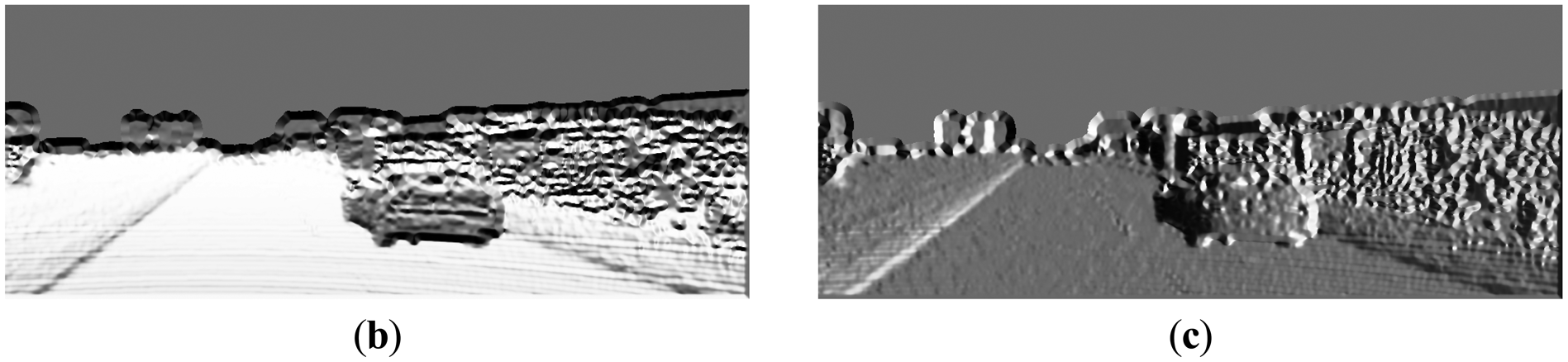
In the edge probability design, we use both the position and the feature. In this subsection, we give a comparison with different probability strategies. One is our method and the other one only uses the position information.
Figure 22 shows a demonstration result: (a) is the visual image of the scene; (b) is the output with only position information; (c) shows our best curb linking results. Because our method includes the curb feature, it successfully tracks the consistent curb points, and filters out isolated noises. Thus our method finally provides better results than the baseline method.
4.3.2. Used Computation Resource
In each step of our method, we take the implementation efficiency into account. The depth recovery and normal estimation take the major part of the computation resource in our method. For depth recovery, we use the Graphic Processing Unit (GPU) implementation from [4], and the processing time for each frame in KITTI is about 30 ms. For normal estimation with depth images, we derive a filter-based method, which only needs some small-size convolutions and pixel-level operations, and the processing time with Central Processing Unit (CPU) is about 15 ms in our experiments. Finally, we achieve 15 Hz (15 frames per second) by using an i7 processor together with a desktop graphics card (NVIDIA GTX260). The total implementation time for each frame in KITTI dataset is about 60 ms, which achieves real-time performance.
4.3.3. The Detection Range
One of the most important advantages of our method is its robustness. By using the dense depth image, our method achieves reliable results even for quite noisy scenes. Our method also achieves larger detection range. In KITTI dataset, in no occlusion condition, the detection range is about +30 m in vertical and +8 m in horizontal for common curbs with about 10 cm height. The typical results are shown in Figures 16a, 17a, 18a, and the statistics results are listed in Table 1.
5. Conclusions and Future Work
In this paper, we have proposed a curb detection method based on fusing the 3D-Lidar and camera data. Using the dense depth image from range-visual fusion, we derived a filter-based method for efficient surface normal estimation. By using the specifically designed pattern of curbs, curb point features were detected in the normal image row by row. We then formulated the curb point linking process as a best path searching on a corresponding Markov Chain, which was solved via dynamic programming. We also designed several post-processing steps to filter the noises, parameterize the curb models and compute their confidence scores. Comprehensive evaluations on KITTI dataset showed that our method achieved good results in both static and dynamic scenes, and processed the data at the speed of 15 Hz. For the obstacle occlusion and strong shadow, our method showed strong robustness. In typical scenes without occlusion, our detection rang reached 30 m for front and 8 m for each side.
In the future, we are going to apply this curb detection method for other ALV applications, such as map building, vehicle localization and so on. To date, there is no widely accepted benchmark for curb detection. A comprehensive benchmark with different sensors for curb detection is needed for fair comparison, and this could be our future work.
Acknowledgments
This work was supported in part by the National Natural Science Foundation of China under Grant Nos. 91220301 and 90820302. The first author would like to acknowledge the financial support from the China Scholarship Council for supporting his visiting research at National University of Singapore, Singapore. The authors would like to acknowledge Jiashi Feng and Li Zhang from National University of Singapore for their advices for this work. The authors would like to acknowledge the reviewers for their constructive and helpful suggestions.
Conflicts of Interest
The authors declare no conflict of interest.
References
- Hervieu, A.; Soheilian, B. Road side detection and reconstruction using LIDAR sensor. Proceedings of 2013 IEEE on the Intelligent Vehicles Symposium (IV), Gold Coast, QLD, Canada, 23–26 June 2013; pp. 1247–1252.
- Aufrere, R.; Mertz, C.; Thorpe, C. Multiple sensor fusion for detecting location of curbs, walls, and barriers. Proceedings of the 2003 IEEE Intelligent Vehicles Symposium, Columbus, OH, USA, 9–11 June 2003; pp. 126–131.
- Michalke, T.; Kastner, R.; Fritsch, J.; Goerick, C. A self-adaptive approach for curbstone/roadside detection based on human-like signal processing and multi-sensor fusion. Proceedings of the 2010 IEEE Intelligent Vehicles Symposium (IV), San Diego, CA, USA, 21–24 June 2010; pp. 307–312.
- Dolson, J.; Baek, J.; Plagemann, C.; Thrun, S. Upsampling range data in dynamic environments. Proceedings of the 2010 IEEE Conference on Computer Vision and Pattern Recognition (CVPR), San Francisco, CA, USA, 13–18 June 2010; pp. 1141–1148.
- Liu, Z.; Wang, J.; Liu, D. A New Curb Detection Method for Unmanned Ground Vehicles Using 2D Sequential Laser Data. Sensors 2013, 13, 1102–1120. [Google Scholar]
- Enzweiler, M.; Greiner, P.; Knoppel, C.; Franke, U. Towards multi-cue urban curb recognition. Proceedings of the 2013 IEEE Intelligent Vehicles Symposium (IV), Gold Coast, QLD, Canada, 23–26 June 2013; pp. 902–907.
- Seibert, A.; Hahnel, M.; Tewes, A.; Rojas, R. Camera based detection and classification of soft shoulders, curbs and guardrails. Proceedings of the 2013 IEEE Intelligent Vehicles Symposium (IV), Gold Coast, QLD, Canada, 23–26 June 2013; pp. 853–858.
- Oniga, F.; Nedevschi, S.; Meinecke, M.M. Curb detection based on a multi-frame persistence map for urban driving scenarios. Proceedings of the 11th International IEEE Conference on Intelligent Transportation Systems (ITSC 2008), Beijing, China, 12–15 October 2008; pp. 67–72.
- Oniga, F.; Nedevschi, S. In Polynomial curb detection based on dense stereovision for driving assistance. Proceedings of the 2010 13th International IEEE Conference on Intelligent Transportation Systems (ITSC), Funchal, Portugal, 19–22 September 2010; pp. 1110–1115.
- Oniga, F.; Nedevschi, S. In Curb detection for driving assistance systems: A cubic spline-based approach. Proceedings of the 2011 IEEE Intelligent Vehicles Symposium (IV), Baden-Baden, Germany, 5–9 June 2011; pp. 945–950.
- Siegemund, J.; Pfeiffer, D.; Franke, U.; Förstner, W. Curb reconstruction using conditional random fields. Proceedings of the 2012 Intelligent Vehicles Symposium, San Diego, CA, USA, 21–24 June 2010; pp. 203–210.
- Siegemund, J.; Franke, U.; Förstner, W. A temporal filter approach for detection and reconstruction of curbs and road surfaces based on conditional random fields. Proceedings of the 2011 IEEE Intelligent Vehicles Symposium (IV), Baden-Baden, Germany, 5–9 June 2011; pp. 637–642.
- Ivanchenko, V.; Shen, H.; Coughlan, J. Elevation-based MRF stereo implemented in real-time on a GPU. Proceedings of the 2009 Workshop on Applications of Computer Vision (WACV), Snowbird, UT, USA, 7–8 December 2009; pp. 1–8.
- Yeonsik, K.; Chiwon, R.; Seung-Beum, S.; Bongsob, S. A Lidar-Based Decision-Making Method for Road Boundary Detection Using Multiple Kalman Filters. IEEE Trans. Ind. Electron. 2012, 59, 4360–4368. [Google Scholar]
- Jaehyun, H.; Dongchul, K.; Minchae, L.; Myoungho, S. Enhanced Road Boundary and Obstacle Detection Using a Downward-Looking LIDAR Sensor. IEEE Trans. Veh. Technol. 2012, 61, 971–985. [Google Scholar]
- El-Halawany, S.; Moussa, A.; Lichti, D.D.; El-Sheimy, N. In Detection of road curb from mobile terrestrial laser scanner point cloud. Proceedings of the ISPRS Workshop on Laserscanning, Calgary, Canada, 29–31 August 2011.
- Maye, J.; Kaestner, R.; Siegwart, R. Curb detection for a pedestrian robot in urban environments. Proceedings of the 2012 IEEE International Conference on Robotics and Automation (ICRA), Saint Paul, MN, USA, 14–18 May 2012; pp. 367–373.
- Zhao, G.; Yuan, J. Curb detection and tracking using 3D-LIDAR scanner. Proceedings of the 2012 19th IEEE International Conference on Image Processing (ICIP), Orlando, FL, USA; 2012; pp. 437–440. [Google Scholar]
- Chen, T.; Dai, B.; Wang, R.; Liu, D. Gaussian-Process-Based Real-Time Ground Segmentation for Autonomous Land Vehicles. J. Intell. Robot. Syst. 2013. [CrossRef]
- Kodagoda, K.; Wijesoma, W.; Balasuriya, A. CuTE: Curb tracking and estimation. Control Syst. Technol. IEEE Trans. 2006, 14, 951–957. [Google Scholar]
- Gallo, O.; Manduchi, R.; Rafii, A. CC-RANSAC: Fitting planes in the presence of multiple surfaces in range data. Pattern Recognit. Lett. 2011, 32, 403–410. [Google Scholar]
- Badino, H.; Huber, D.; Park, Y.; Kanade, T. Fast and accurate computation of surface normals from range images. Proceedings of the 2011 IEEE International Conference on Robotics and Automation (ICRA), Shanghai, China, 9–13 May 2011; pp. 3084–3091.
- Lin, H.; Kim, H.; Lin, C.-S.; Chua, L.O. Road boundary detection based on the dynamic programming and the randomized hough transform. International Symposium on Information Technology Convergence (ISITC 2007), Washington, DC, USA; 2007; pp. 63–70. [Google Scholar]
- Adhikari, S.P.; Kim, H. Dynamic programming and curve fitting based road boundary detection. In In Proceedings of the 9th WSEAS International Conference on Computational Intelligence, Man-Machine Systems and Cybernetics, 2010; World Scientific and Engineering Academy and Society (WSEAS): Stevens Point, WI, USA, 2010; pp. 236–240. [Google Scholar]
- Geiger, A.; Lenz, P.; Stiller, C.; Urtasun, R. Vision meets robotics: The KITTI dataset. Int. J. Robot. Res. 2013, 32, 1231–1237. [Google Scholar]


| Experiments | Sides | Detection Range (meters) | Scores | |||
|---|---|---|---|---|---|---|
| Min(XW) | Max(XW) | Min(YW) | Max(YW) | |||
| Figure 16a | Left | −6.19 | −4.99 | 6.08 | 27.58 | 24.93 |
| Right | 0.99 | 1.34 | 6.26 | 30.63 | 30.30 | |
| Figure 16b | Left | −5.47 | −5.28 | 8.05 | 15.63 | 19.58 |
| Right | 0.47 | 0.79 | 7.43 | 30.19 | 62.14 | |
| Figure 17a | Left | −8.41 | −7.89 | 10.88 | 25.04 | 12.89 |
| Right | 3.65 | 4.72 | 6.52 | 32.93 | 42.16 | |
| Figure 17b | Left | −2.33 | −2.01 | 5.86 | 28.14 | 38.60 |
| Right | 1.42 | 2.47 | 6.06 | 16.16 | 18.08 | |
| Figure18a | Left | −6.55 | −5.17 | 6.88 | 30.78 | 46.43 |
| Right | 3.43 | 5.06 | 6.31 | 30.30 | 46.24 | |
| Figure 18b | Left | −5.84 | −5.39 | 6.50 | 19.28 | 26.17 |
| Right | 0.97 | 1.11 | 6.38 | 10.71 | 36.69 | |
| Figure 19a | Left | −4.90 | −4.67 | 6.51 | 11.53 | 33.47 |
| Right | 2.51 | 4.07 | 5.72 | 28.63 | 24.47 | |
| Figure 19b | Left | −4.11 | 5.56 | 6.48 | 22.98 | 28.39 |
| Right | 3.76 | 13.21 | 6.60 | 22.62 | 63.25 | |
| Figure 20a | Left | −5.92 | −4.77 | 6.19 | 20.48 | 43.45 |
| Right | 0.99 | 1.13 | 5.94 | 8.79 | 17.93 | |
| Figure 20b | Left | −4.00 | −3.45 | 6.23 | 20.06 | 32.06 |
| Right | - | - | - | - | 0 | |
| Figure 21a | Left | −5.98 | −4.27 | 6.55 | 12.68 | 25.76 |
| Right | - | - | - | - | 0 | |
| Figure 21b | Left | −5.63 | −4.29 | 6.31 | 12.48 | 29.11 |
| Right | 0.24 | 1.43 | 8.70 | 14.14 | 21.30 | |
© 2014 by the authors; licensee MDPI, Basel, Switzerland. This article is an open access article distributed under the terms and conditions of the Creative Commons Attribution license ( http://creativecommons.org/licenses/by/3.0/).
Share and Cite
Tan, J.; Li, J.; An, X.; He, H. Robust Curb Detection with Fusion of 3D-Lidar and Camera Data. Sensors 2014, 14, 9046-9073. https://doi.org/10.3390/s140509046
Tan J, Li J, An X, He H. Robust Curb Detection with Fusion of 3D-Lidar and Camera Data. Sensors. 2014; 14(5):9046-9073. https://doi.org/10.3390/s140509046
Chicago/Turabian StyleTan, Jun, Jian Li, Xiangjing An, and Hangen He. 2014. "Robust Curb Detection with Fusion of 3D-Lidar and Camera Data" Sensors 14, no. 5: 9046-9073. https://doi.org/10.3390/s140509046