A Stochastic Approach to Noise Modeling for Barometric Altimeters


Abstract
: The question whether barometric altimeters can be applied to accurately track human motions is still debated, since their measurement performance are rather poor due to either coarse resolution or drifting behavior problems. As a step toward accurate short-time tracking of changes in height (up to few minutes), we develop a stochastic model that attempts to capture some statistical properties of the barometric altimeter noise. The barometric altimeter noise is decomposed in three components with different physical origin and properties: a deterministic time-varying mean, mainly correlated with global environment changes, and a first-order Gauss-Markov (GM) random process, mainly accounting for short-term, local environment changes, the effects of which are prominent, respectively, for long-time and short-time motion tracking; an uncorrelated random process, mainly due to wideband electronic noise, including quantization noise. Autoregressive-moving average (ARMA) system identification techniques are used to capture the correlation structure of the piecewise stationary GM component, and to estimate its standard deviation, together with the standard deviation of the uncorrelated component. M-point moving average filters used alone or in combination with whitening filters learnt from ARMA model parameters are further tested in few dynamic motion experiments and discussed for their capability of short-time tracking small-amplitude, low-frequency motions.1. Introduction
Barometric altimeters can be used for measuring the height of an object above a given reference level, e.g., the sea level—a popularly used term for this height is pressure altitude. Common applications are, e.g., in avionics, where barometric altimeters can help in stabilizing the vertical position and velocity of a flying object [1,2]. Recently, barometric altimeters have been considered for interesting human-centric applications, such as personal navigation and human motion tracking and monitoring. Beside their use as wristop computers for leisure and sports, barometric altimeters were integrated within multi-sensor pedestrian navigation systems and activity monitors, for improving performance of dead-reckoning algorithms or classifiers of human motion patterns: e.g., they were used to detect the moving styles of going up/down the stairs or in an elevator [3]; to determine the correct floor of a user in a multi-storey building [4]; to detect stair ascent-descent in ambulatory monitors designed for estimating the energy expenditure incurred during activities of daily living, including stair-walking [5,6]. More recently, it was proposed that the measured pressure altitudes might help improving accelerometry-based fall detection systems [7–10]. The rationale behind this application is that, when a person is standing, the difference in atmospheric air pressure between the waist and the feet can be monitored for sudden changes that would indicate a fall event [7]. However, rapid changes in pressure uncorrelated with altitude can be generated, outdoors, by unpredictable atmospheric conditions, and, indoors, by frequent opening/closing of windows or doors and by air conditioning systems [11]. The consequence is that barometric altimeter data tends to be very noisy, and their accuracy is rather poor.
Recent advances in MEMS sensing technologies have led to the availability of barometric altimeters that are well suited for integration in mobile and portable systems. The most popular barometric altimeters for human-centric applications are manufactured by Bosch Sensortec (Reutlingen, Germany) [8–12] and VTI Technologies (Vantaa, Finland) [6,7,9]. These sensors can be used in few measurement modes, which differ in the resolution offered for a given sampling rate. Published recipes for pressure altitude signal conditioning and pre-processing do not go beyond generic prescriptions for low-pass filtering, e.g., in order to obtain an accuracy of 0.1 m using the barometric altimeter alone, several seconds of averaging would be necessary [12].
In this paper we develop a method for capturing salient statistical properties of the noise that affects barometric altimeters (stochastic approach to noise modeling). Using the developed model we intend to assess the short-time tracking performance of small-amplitude, low-frequency motions. By the term short-time motion tracking we refer to motions with durations up to few minutes, in which relative changes of altitude are to be tracked. Conversely, long-time motion tracking involves accurate tracking of absolute altitude over long time intervals. In human-centric applications, both tracking modes are involved: short-time tracking, e.g., fall detection; long-time tracking, e.g., personal navigation. Under conditions of short-time motion tracking, the time-varying mean is expected to vary very slowly, contributing an offset in the measured pressure altitude with no practical effect on the tracking accuracy. In those applications where accurate absolute altitude is needed, barometric altimeters in differential mode are perhaps the best option available to deal with slow changes of atmospheric pressure [11].
The proposed method of analysis decomposes the noise in three additive components with different physical origin and properties: a deterministic time-varying mean, correlated with slow pressure changes that can be involved in, e.g., local weather forecasting [13] and long-time tracking [14], whose modeling is beyond the scope of this paper; an exponentially time-correlated random process, modeled as a first-order Gauss-Markov (GM) process, that accounts for short-term, local environment changes, whose effect is prominent for short-time tracking; an uncorrelated random process, mainly due to wideband electronic noise, including quantization noise. We take the novel approach of using Gauss Markov (GM) random processes for modeling the short-time correlated component of altimeter noise. The reason for this choice is that GM random processes are mathematically simple, with only a limited number of parameters that need to be estimated [15]. Moreover, they seem to fit a wide variety of physical phenomena with reasonable accuracy [16]. Autoregressive-moving average (ARMA) system identification techniques are used to capture the correlation structure of the piecewise stationary GM component, and to estimate its standard deviation, together with the standard deviation of the uncorrelated component.
Experimental results obtained when the barometric altimeter is either motionless (for model identification) or moving (for tracking performance assessment) are presented. To this aim M-point moving average filters are applied to time-correlated pressure altitude signals, alone or cascaded with whitening filters learnt from ARMA model parameters. Advantages and disadvantages of removing the short-term correlation of the GM component by whitening filters are discussed.
2. Methods
2.1. Measurement Process
The International Standard Atmosphere (ISA) model can be used to calculate the altitude from the output of an air pressure sensor [17]. The basic physical equations used for modeling the atmosphere are the hydrostatic equation:
Equations (1) and (2) can be combined together yielding the first-order differential equation:
The assumption of constant gravity is not crucial in solving Equation (3), that is, the variation of gravity with altitude and latitude can be safely ignored for short-distance trips [18]. Moreover, it is known that temperature tends to change with altitude. The lapse rate is defined as the rate of temperature increase in the atmosphere with the altitude: a constant lapse rate L can be assumed between 0 and 11 km (L = −6.5 K/km)—the negative sign indicates that the temperature decreases with altitude.
Equation (3) can be solved under the assumption of constant gravity and lapse rate, yielding the barometric formula:
The ISA model fails to accurately describe the real atmosphere in many ways. The assumption of hydrostatic equilibrium is generally valid, provided that the effects of short-term winds can be tolerated. In the real atmosphere significant variations are also observed in pressure, temperature and even lapse rate. Moreover, although the ideal gas assumption is highly accurate for air, the behavior of an ideal gas is influenced by R̅ the value of which depends in turn on mean molecular weight. The composition of the lower atmosphere is approximately constant, but in a very wet atmosphere the water vapor content can be high enough to significantly lower the density of the air, thus changing the value of R̅.
Absolute altitude information cannot be easily obtained; in particular, it is necessary to know, inter alia, the local sea level pressure, which may differ from standard pressure. Equation (4) still applies in cases where the pressure and the temperature differ from those of the standard: the relative change in pressure and the actual temperature determine the change in altitude regardless of altitude. Fortunately, it is the change in altitude to be important in, e.g., human-centric applications including fall detection. To overcome difficulties in matching the ISA model to real atmospheric conditions, the use of a reference barometric altimeter at a known and constant altitude has been also proposed to obtain altitude from a moving barometric altimeter (differential barometry), although local disturbances in pressure were critical for achieving high accuracy [11].
2.2. Stochastic Approach to Noise Modeling
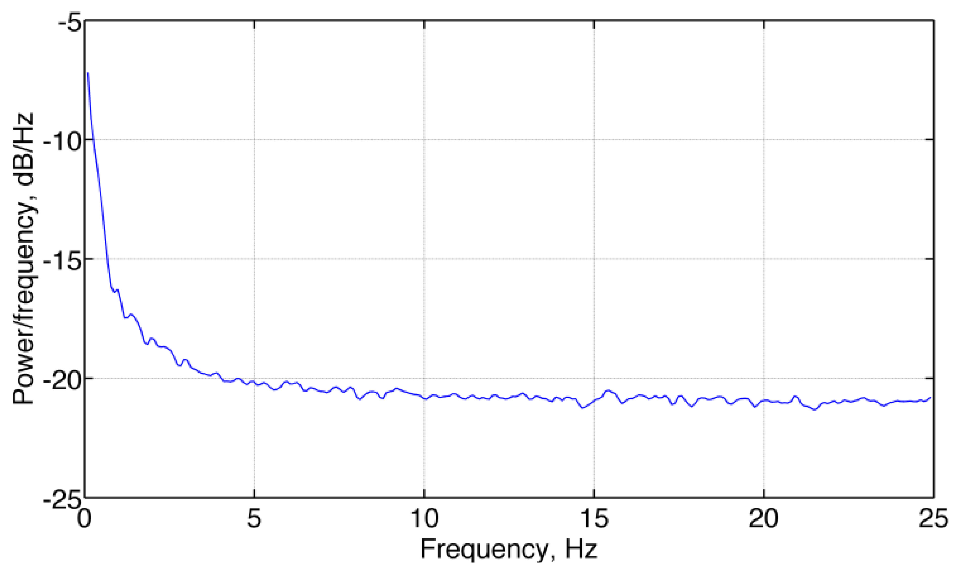
Figure 1 shows a typical portrait of the spectrum of barometric altimeter noise (pressure altitude). The concentration of noise energy in the low frequency region of the spectrum (colored noise) can be explained as the consequence of, e.g., thermal gradients and air flow in the sensor vicinity.
In this paper the noise n(t) superimposed to the output of a barometric altimeter is assumed to be the additive combination of three different components:
nc(t) is produced from passing a white Gaussian driving noise with zero-mean and unit variance through a first-order shaping filter with frequency response:
The standard deviation σc at the output of the shaping filter Equation (6) is given by:
nu(t) can be described in a similar fashion. The zero-order shaping filter can be approximated over the sensor bandwidth as follows:
The standard deviation σu is therefore given by:
Applying the spectral factorization technique to the additive combination of the spectral densities of nc(t) and nu(t), which are assumed independent, the following expression of the overall shaping filter is obtained:
Since the pressure altitude samples from the barometric altimeter are available only at discrete times that are integer multiples of the sampling interval Ts, the shaping filter Equation (10) is discretized using the bilinear transform technique, yielding:
Equations (7), (9), (11), (13), (14) allow us to compute σc, σu and τ from Ho, a, and b. For example, the correlation time constant is given by:
Using autoregressive moving average (ARMA) system identification techniques, Ho, a, and b can be estimated from air pressure signals that were previously detrended by subtracting the time-varying mean.
Under the assumption that the shaping filter Equation (12) is identified using the ARMA(1,1) model structure and the prediction-error approach to parameter estimation [15], the asymptotic covariance matrix of the estimates ae and be of the parameters a and b is given by [19]:
The estimates returned by the prediction-error approach are known to be asymptotically normally distributed as the number N of data samples tends to infinity. However, σc, σu and τ are non-linearly related to Ho, a, and b. Departures from Gaussianity can then be observed in the distributions of the estimates of σc, σu and for any finite N. The problem is especially acute for the correlation time constant: not surprisingly, since estimating the correlation time constant of a GM random process is known to require a relatively huge amount of data for accurate results [20].
The experimental distribution of τ turns out to be right-skewed, since the estimated value of the model pole is close to the unit circle. For a given observation period, as needed to preserve the short-term stationarity, the attempts to improve the estimation accuracy by increasing N are counterweighted by the decrease of the sampling interval, with a consequent shift of the model pole toward the critical point z = 1.
2.3. Sensor Hardware
The experiments described in this paper were performed using a battery-powered wearable inertial measurement unit (WIMU) whose development is undergoing in our lab for applications in human motion ambulatory monitoring and assessment. The WIMU is endowed with a 32-bit ARM Cortex processor (LPC1768, NXP Semiconductors, Eindhoven, the Netherlands) and a Bluetooth transceiver for data communication with an Android-based smart-phone (Samsung Galaxy SII, GT-I9100, Samsung, Seoul, South Korea). The WIMU sensors are a digital tri-axial gyro (ITG-3200, InvenSense, San Jose, CA, USA), a digital tri-axial accelerometer (BMA180, Bosch, Reutlingen, Germany), a digitaltri-axial magnetic sensor (HMC5843, Honeywell, Morristown, NJ, USA), and a digital pressure sensor (Bosch BMP085).
The measurements by the BMP085 digital pressure sensor are noisy, including a significant amount of quantization noise due to a coarse resolution of about 1 Pa (corresponding to about 8.43 cm). The BMP085 was used in the ultra-low power mode (no oversampling was performed internally to the sensor). The ANSI C code by the sensor manufacturer was used to implement the compensation algorithm for pressure and temperature measurement using the integrated thermal sensor [21]. We ported this piece of software to the ARM controller of the WIMU, together with the routine for calculating the altitude from calibrated pressure measurements using Equation (4). The temperature was measured once per second, and this value was used for all pressure altitude measurements during the same period. Pressure altitude data were computed by the ARM controller of the WIMU and logged to the smart-phone at a rate of 50 Hz, before their upload to a PC for subsequent analysis.
2.4. Experiments
The barometric altimeter was tested in static and motion conditions. The barometric altimeter was motionless on a table while six data acquisition trials, each of one lasting 10 min, were performed in different day hours, either in a household environment or outdoors (tests in static conditions). The testing procedure was repeated a second time, days later, in similar environmental conditions as above. Static tests allowed ARMA model identification and validation. Based on the ARMA model parameters, a whitening filter was also designed by inverting and discretizing the shaping filter Equation (10), as explained in the next subsection.
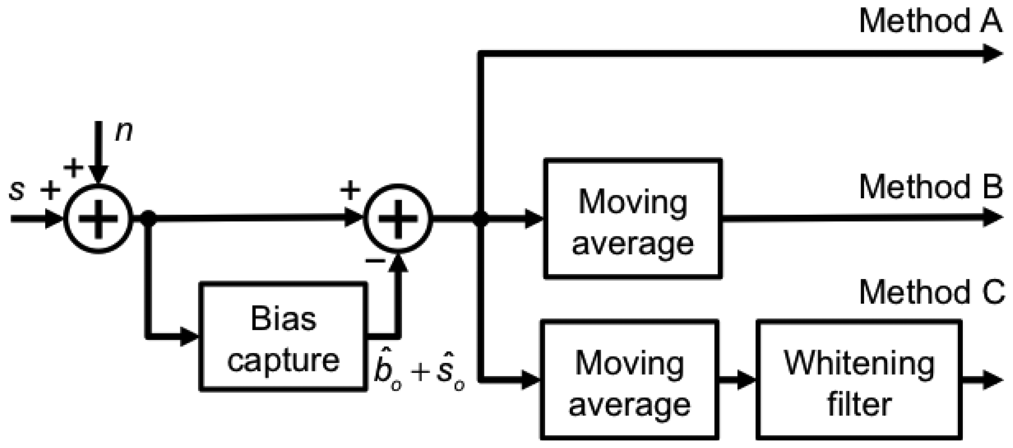
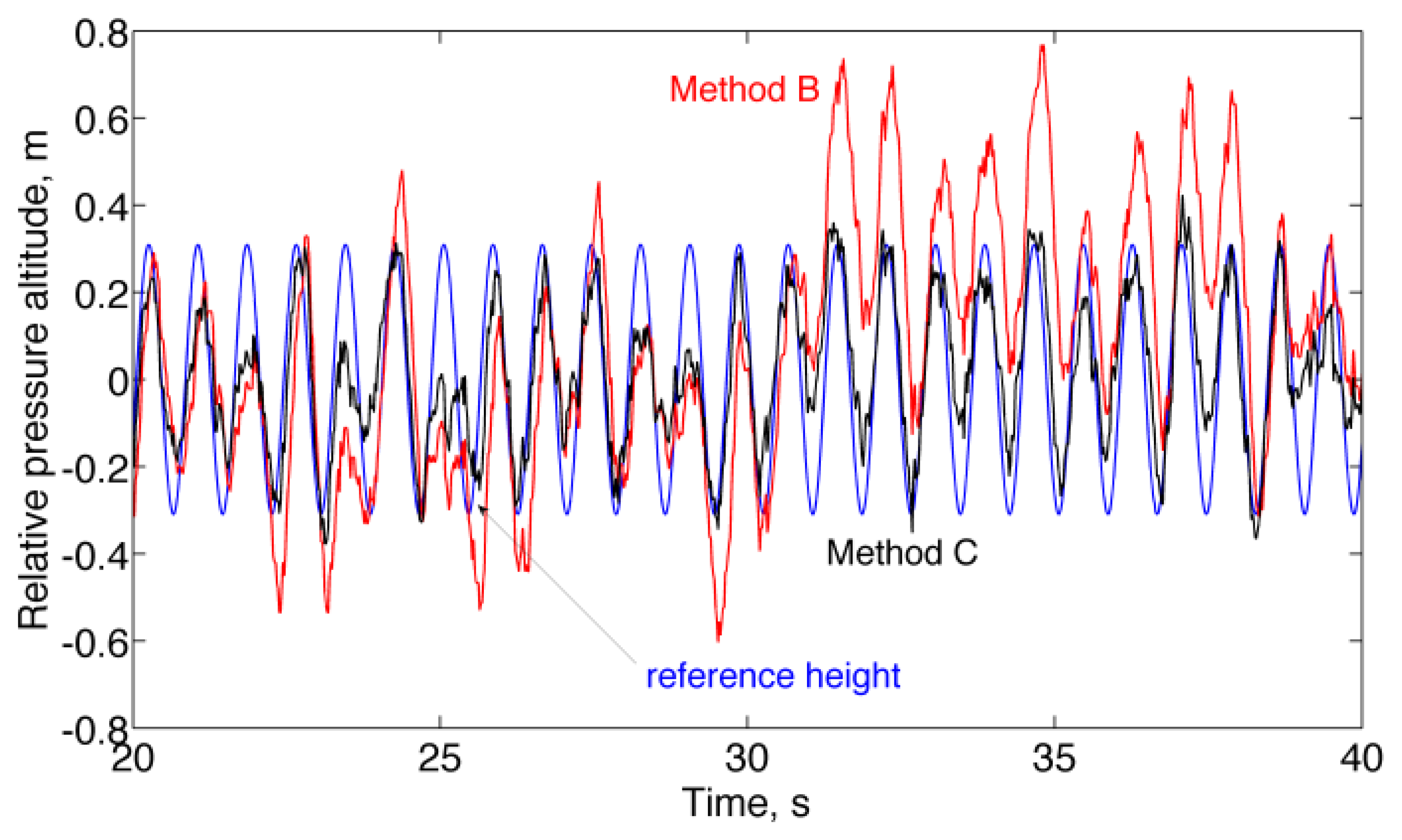
Two motion tracking experiments were also performed (tests in motion conditions). These experiments with a moving barometric altimeter were used to test few methods of signal processing: Method A (no filtering); Method B (4-point moving average filtering); Method C (4-point moving average filtering cascaded with the designed whitening filter). In the first experiment, the WIMU was mounted at the waist of a person who walked indoors along stairs spanning 1.7 m for each floor in a series of three distinct floors from ground level (stair-walking). During the second motion tracking experiment (forced circular motion), the WIMU was affixed at the distal part of a plastic rod; the rod was hinged on the axis of an electric motor controlled in rotation speed using a user interface running on a PC. The rod was lying in a plane aligned to gravity, so as the barometric altimeter traced a circle of radius 30 cm; the rod was rotated for two minutes at each of four different motion frequencies, 0.25, 0.5, 1, and 1.5 Hz. The measurement data (pressure altitude from the barometric altimeter and rod angular position by the incremental encoder fitted to the motor axis) were electrically synchronized and logged to the host computer for further analysis. The vertical position of the barometric altimeter relative to its initial position was estimated using the encoder measurements and the known length of the rod, yielding the reference against which the relative change in pressure altitude estimated by the barometric altimeter was compared for Root Mean Square Error (RMSE) analysis.
During motion tracking experiments, the relative pressure altitude was computed by taking the average value of the absolute pressure altitude b̂o + ŝo during a rest period of 1 s before the motion started; the absolute pressure altitude signals were then detrended by subtracting this constant value from them (bias capture), Figure 2.
2.5. Data Processing for ARMA System Identification
Data processing was carried out using MATLAB. Piecewise constant fitting of raw data from static tests was performed using data windows of fixed size (1 min), and data were locally detrended by subtracting the constant level (detrended raw data). After applying a 4-point moving average filter, the filtered data were downsampled by 5 (Ts = 0.1 s), in preparation for ARMA system identification, Figure 3.
ARMA model parameters were then estimated for each non-overlapping data window of N = 300 data samples (i.e., 30 s) using the prediction-error approach. The adequacy of the fitted model was assessed applying the Bartlett's test of whiteness to the prediction-error sequence at the 95% level. The Akaike's final prediction error criterion was used to defend the ARMA(1,1) model against higher-order models.
The sampling interval and the window length were chosen with the aim to reduce the model parameter uncertainty while preserving the short-term stationarity of the processed data. The short-term stationarity was assessed using the spectral error measure approach [15]. The model parameters values were averaged (10% trimmed mean) and the standard deviation (SD) was computed on the trimmed values—the reason for trimming was to reject outliers that were observed, especially when the correlation time constant was estimated. Once the model was successfully identified and validated, the shaping filter Equation (10) was inverted and discretized using the bilinear transform technique at the sampling frequency of 50 Hz (whitening filter). The detrended raw data were then filtered using the 4-point moving average cascaded with the whitening filter and the procedure of model identification was applied to time-decimated filtered data. In principle, the whitening filter generates surrogate data where the serial correlation present in the input data is removed. When ARMA system identification was applied to surrogate data, zero-pole cancellation was verified by testing the null hypothesis that the difference between ae and be was null (paired sample t-test, p > 0.1). The standard deviation of the uncorrelated noise component was computed as σu = Ho.
3. Results
3.1. ARMA Model Identification and Validation
Tables 1 and 2 report the 10% trimmed mean value ± SD of σc, σu and τ for the experiments in static conditions of the first and second day, respectively. The last column gives the total standard deviation σs of the pressure altitude signals.
The standard deviation of the correlated noise component took higher values than in relatively unperturbed conditions, while the standard deviation of the uncorrelated noise component was relatively unchanged. Figure 4 reports a representative plot of measured pressure altitude.
A one-way analysis of variance was performed for comparing the means of the six groups of point estimates of a and b from the experiments during the first day. The null hypothesis that the means of the groups were equal was accepted, yielding: ae = −0.86 ± 0.03 (p > 0.4), and be = −0.52 ± 0.06 (p > 0.26)—the agreement with the estimation uncertainty computed theoretically from Equation (16) was also very good. The whitening filter designed using these point estimates had a pole at a frequency of about 1 Hz, a zero approximately two octave down; a unity-gain constraint was enforced at 25 Hz, yielding a DC gain of about 0.21.
Surrogate data were generated by applying the whitening filter to the detrended raw data from both days. Surrogate data were submitted to ARMA identification after 4-point moving average filtering and time decimation, as described above. Zero-pole cancellation took place, even when the whitening filter was applied to data from the second day, which means that the whitening filter was effective in removing serial correlation from surrogate data, Tables 3 and 4. The last column gives the total standard deviation σs of the whitened pressure altitude signals.
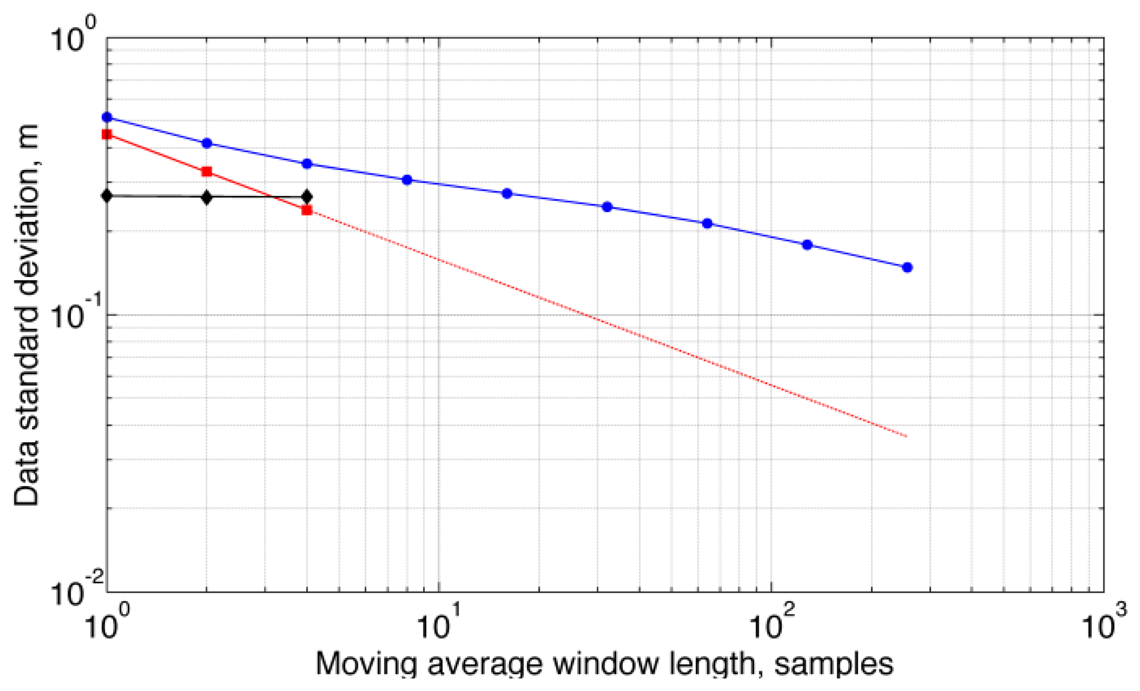
Detrended raw data from static tests were also submitted to ARMA identification when M-point moving average filtering was applied for dyadic values of M, Figure 5. Due to frequent failures of the Bartlett's test of whiteness, the ARMA(1,1) model was unable to fit the data for M ≥ 8.
3.2. Motion Tracking Tests
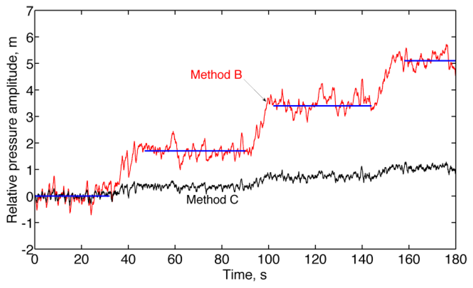
Finally, the results of the experiments in motion conditions are presented in Figure 6 and Table 5 (stair-walking), Figure 7 and Table 6 (forced circular motion). For better readability of the plots, the raw relative pressure altitudes (Method A) are not reported in Figures 6 and 7.
4. Discussion
One important result from using the method of analysis developed in this paper is that the generic prescription that several seconds of averaging of barometric altimeter data are necessary to achieve accuracy in the order of 0.1 m is quite misleading. The correlated noise component should be accounted when assessing the benefits of averaging. In all performed static tests, either indoors or outdoors, the correlated noise component turned out to have a greater standard deviation than the uncorrelated noise component, Tables 1 and 2, raising concerns about the suitability of, e.g., moving average filters to reduce altimeter noise.
The correlated noise component was virtually unaffected by an M-point moving average filter when M ≥ 4 at a sampling frequency of 50 Hz, and its standard deviation would decrease very slowly for higher values of M, although it was not possible to estimate the ARMA(1,1) model parameters for M ≥ 8, Figure 5. This was due to the fact that data fitting would include the M-point moving average filter itself, which called for higher-order ARMA models. The behavior of the total standard deviation shows that the scaling law, valid for uncorrelated data, is optimistic when dealing with time-correlated data [22]. A noise level of 0.15 cm was reached only when M = 256, which corresponds to an averaging time of about 5 s and a delay of 2.5 s in the filtering chain; on the other hand, M = 32 would suffice to reach a noise level of 0.1 cm if only uncorrelated noise would be present in the barometric altimeter output (however, M = 32 is equivalent to a delay in the filtering chain of 320 ms that can be unacceptably high in several human-centric applications, e.g., pre-impact fall detection [23]).
The whitening filter was a highly effective tool for filtering the correlated noise component, as shown by the results reported in Tables 3 and 4. However, a problem with its use in dynamic motion experiments was related to where the unity-gain constraint was enforced. Since the correlated noise component occupies the low-frequency part of the spectrum, the whitening filter presents a typically high-pass frequency response, which tends to amplify uncorrelated noise unless the unity-gain constraint is moved from DC to higher frequencies. Accurate height tracking would then be possible for dynamic motion frequencies exceeding, say, few Hertz; unfortunately, typical vertical human motions, such as walking up or down a staircase, have motion frequencies much smaller than the −3 dB corner frequency of the whitening filter. The amplifying effect on the uncorrelated noise component due to a unity-gain constraint enforced at DC would require, approximately, a 25-fold increase in the length of the M-point moving average filter for achieving the same Signal-to-Noise ratio, which is untenable in practice.
The results of the stair-walking experiment clearly show the difficulty of placing the unity-gain constraint at high frequency (Figure 6 and Table 5). The pressure altitude change from one floor to the next floor was underestimated, on average, by a factor close to the whitening filter DC gain when Method C was used, as compared to Method B, at the expense of much smaller fluctuations around the mean value. The advantages of using the whitening filter can be seen when analyzing the results of the forced circular motion experiment (Figure 7 and Table 6), in which the motion frequencies were higher than in the stair-walking experiment.
5. Conclusions
In this paper we have developed a method of analysis of barometric altimeter noise based on system identification techniques. Beside the slowly time-varying mean, which was outside our scope in the present context, the noise-like fluctuations on barometric altimeter output were interpreted as the superposition of a GM random process that explained short-term temperature and pressure changes (environment-dependent) and an uncorrelated noise component with relatively time-invariant statistics, which accounted for electronics noise. Based on the ARMA model parameters, a whitening filter was also designed and tested, together with standard M-point moving average filters, for improving short-time tracking of small-amplitude, low-frequency motions.
Because of their limited accuracy, it is presently a matter of debate whether barometric altimeters can be effectively used in human-centric applications, e.g., fall detection. It is likely that they will find their role as aiding sensors in systems where multi-sensor fusion methods for motion tracking and event detection are implemented. Oftentimes, these methods are optimal when the sensor noise is white, and their robustness may be an issue when the whiteness assumption is not valid [24]. The developed method can thus be used in building simulation environments for algorithm testing, as well as in providing practical tools, e.g., whitening filters, by means of which the performance of a given signal processing method can be improved. Moreover, the developed method can be used to perform a sort of environment probing, namely local environmental effects can be directly gauged in terms of the percentage of the total variance due to noise in barometric altimeters.
Acknowledgments
This work was partly supported by the Italian Ministry of Education and Research (MIUR) through the relevant interest national project (PRIN) “A quantitative and multi-factorial approach for estimating and preventing the risk of falls in the elderly people”, and by the EC funded project I-DONT-FALL “Integrated prevention and Detection sOlutioNs Tailored to the population and Risk Factors associated with FALLs” (CIP-ICT-PSP-2011-5-297225). The views expressed in this paper are not necessarily those of the I-DONT-FALL consortium. The authors are grateful to Andrea Mannini for his valuable help in setting up the forced circular motion experiment.
Conflicts of Interest
The authors declare no conflict of interest.
References
- Hsiao, F.-B.; Liu, T.-L.; Chien, Y.-H.; Lee, M.-T.; Hirst, R. The development of a target-lock-on optical remote sensing system for unmmaned aerial vehicles. Aeronaut. J. 2006, 110, 163–172. [Google Scholar]
- van der Merwe, R.; Wan, E.A.; Julier, S.I. Sigma-Point Kalman Filters for Nonlinear Estimation and Sensor-Fusion Applications to Integrated Navigation. Proceedings of Collection of Technical Papers—AIAA Guidance, Navigation, and Control Conference, Providence, RI, USA, 16–19 August 2004; pp. 1735–1764.
- Sagawa, K.; Ishihara, T.; Ina, A.; Inooka, H. Classification of Human Moving Patterns Using Air Pressure and Acceleration. Proceedings of 24th Annual Conference of the IEEE Industrial Electronics Society, Aachen, Germany, 31 August–4 September 1998; pp. 1214–1219.
- Retscher, G. Altitude Determination of a Pedestrian in a Multi-Storey Building. In Location based services and telecartography; Gartner, G., Cartwright, W.E., Peterson, M.P., Eds.; Springer-Verlag: Berlin/Heidelberg, Germany, 2007; pp. 119–130. [Google Scholar]
- Ohtaki, Y.; Susumago, M.; Suzuki, A.; Sagawa, K.; Nagatomi, R.; Inooka, H. Automatic classification of ambulatory movements and evaluation of energy consumptions utilizing accelerometers and a barometer. Microsyst. Technol. 2005, 11, 1034–1040. [Google Scholar]
- Voleno, M.; Redmond, S.J.; Cerutti, S.; Lovell, N.H. Energy Expenditure Estimation Using Triaxial Accelerometry and Barometric Pressure Measurement. Proceedings of Annual International Conference of the IEEE Engineering in Medicine and Biology Society (EMBC), Buenos Aires, Argentina, 31 August–4 September 2010; pp. 5185–5188.
- Bianchi, F.; Redmond, S.J.; Narayanan, M.R.; Cerutti, S.; Lowell, N.H. Barometric pressure sensors and triaxial accelerometry-based falls event detection. IEEE Trans. Neural Syst. Rehab. Eng. 2010, 18, 619–627. [Google Scholar]
- Salomon, R.; Lüder, M.; Gerald, B. iFall—A New Embedded System for the Detection of Unexpected Falls. Proceedings of 8th IEEE International Conference on Pervasive Computing and Communications Workshops, Mannheim, Germany, 29 March–2 April 2010; pp. 286–291.
- Tolkiehn, M.; Atallah, L.; Lo, B.; Yang, A.Y. Direction Sensitive Fall Detection Using a Triaxial Accelerometer and a Barometric Pressure Sensor. Proceedings of 33th Annual International Conference of IEEE Engineering in Medicine and Biology Society, Boston, MA, USA, 30 August–3 September 2011; pp. 369–372.
- Leuenberger, K.; Gassert, R. Low-Power Sensor Module for Long-Term Activity Monitoring. Proceedings of 33th Annual International Conference of IEEE Engineering in Medicine and Biology Society, Boston, MA, USA, 30 August–3 September 2011; pp. 2237–2241.
- Parviainen, J.; Kantola, J.; Collin, J. Differential Barometry in Personal Navigation. Proceedings of IEEE/ION Position, Location and Navigation Symposium, Monterey, CA, USA, 5–8 May 2008; pp. 148–152.
- Tanigawa, M.; Luinge, H.J.; Schipper, L.J.; Slycke, P.J. Drift-Free Dynamic Height Sensor Using MEMS IMU Aided by MEMS Pressure Sensor. Proceedings of 5th Workshop on Positioning, Navigation and Communication, Hannover, Germany, 27–28 March 2008; pp. 191–196.
- SCP1000-D01/D11 Pressure Sensor as Barometer and Altimeter. In VTI Technologies, Application Note 33. Available online: http://www.maxentropy.net/stamp/SCP1000/ (accessed on 22 October 2013).
- Seo, J.; Lee, J.G.; Park, C.G. Bias Suppression of GPS Measurement in Inertial Navigation System Vertical Channel. Proceedings of IEEE/ION Position, Location and Navigation Symposium, Monterey, CA, USA, 26–29 April 2004; pp. 143–147.
- Sabatini, A.M. A stochastic model of the time of flight noise in airborne sonar ranging systems. IEEE Trans. Ultrason. Ferroelectr. Freq. Control 1997, 44, 606–614. [Google Scholar]
- Brown, R.G.; Hwang, P.Y.C. Introduction to Random Signals and Applied Kalman Fitering; John Wiley & Sons: New York, NY, USA, 1997. [Google Scholar]
- Talay, T.A. SP-367 Introduction to the Aerodynamics of Flight. Available online: http://history.nasa.gov/SP-367/contents.htm (accessed on 22 October 2013).
- Blanchard, R.L. A new algorithm for computing inertial altitude and vertical velocity. IEEE Trans. Aerosp. Electron. Syst. 1971, 7, 1143–1146. [Google Scholar]
- Box, G.E.P.; Jenkins, G.M. Time Series Analysis; Holden-Day: Oakland, CA, USA, 1976. [Google Scholar]
- Bendat, J.S.; Piersol, A.G. Random Data: Analysis and Measurement Procedures, 4th ed.; John Wiley & Sons: Hoboken, NJ, USA, 2010. [Google Scholar]
- BMP085 Digital Pressure Sensor. Available online: ( http://www.adafruit.com/datasheets) (accessed on 22 October 2013).
- Schmelling, M. Averaging correlated data. Phys. Scr. 1995, 51, 676–679. [Google Scholar]
- Wu, G.; Xue, S. Portable preimpact fall detector with inertial sensors. IEEE Trans. Neural Syst. Rehab. Eng. 2008, 16, 178–183. [Google Scholar]
- Maybeck, P.S. Stochastic Models, Estimation and Control; Academic Press Inc.: New York, NY, USA, 1982. [Google Scholar]


| τ, s | σc, m | σu, m | σs, m | |
|---|---|---|---|---|
| Indoors static tests | ||||
| 1 | 0.71 ± 0.27 | 0.26 ± 0.03 | 0.23 ± 0.01 | 0.33 ± 0.03 |
| 2 | 0.87 ± 0.34 | 0.27 ± 0.04 | 0.24 ± 0.01 | 0.34 ± 0.03 |
| 3 | 0.72 ± 0.21 | 0.26 ± 0.02 | 0.23 ± 0.01 | 0.33 ± 0.02 |
| Outdoors static tests | ||||
| 1 | 0.77 ± 0.30 | 0.26 ± 0.03 | 0.24 ± 0.01 | 0.34 ± 0.02 |
| 2 | 0.68 ± 0.32 | 0.29 ± 0.02 | 0.24 ± 0.01 | 0.36 ± 0.04 |
| 3 | 0.65 ± 0.23 | 0.27 ± 0.03 | 0.23 ± 0.01 | 0.34 ± 0.03 |
| τ, s | σc, m | σu, m | σs, m | |
|---|---|---|---|---|
| Indoors static tests | ||||
| 1 | 0.69 ± 0.32 | 0.27 ± 0.04 | 0.24 ± 0.01 | 0.35 ± 0.04 |
| 2 | 0.82 ± 0.23 | 0.27 ± 0.05 | 0.25 ± 0.01 | 0.35 ± 0.04 |
| 3 | 0.78 ± 0.36 | 0.29 ± 0.05 | 0.27 ± 0.01 | 0.38 ± 0.05 |
| Outdoors static tests | ||||
| 1 | 0.75 ± 0.34 | 0.24 ± 0.03 | 0.22 ± 0.01 | 0.32 ± 0.03 |
| 2 | 1.26 ± 0.39 | 0.29 ± 0.03 | 0.23 ± 0.01 | 0.34 ± 0.04 |
| 3 | 0.98 ± 0.26 | 0.28 ± 0.04 | 0.25 ± 0.03 | 0.36 ± 0.05 |
| τ, s | σc, m | σu, m | σs, m | |
|---|---|---|---|---|
| Indoors static tests | ||||
| 1 | -- | -- | 0.22 ± 0.02 | 0.24 ± 0.01 |
| 2 | -- | -- | 0.23 ± 0.02 | 0.24 ± 0.01 |
| 3 | -- | -- | 0.22 ± 0.02 | 0.23 ± 0.01 |
| Outdoors static tests | ||||
| 1 | -- | -- | 0.22 ± 0.03 | 0.25 ± 0.01 |
| 2 | -- | -- | 0.23 ± 0.02 | 0.25 ± 0.01 |
| 3 | -- | -- | 0.21 ± 0.03 | 0.24 ± 0.01 |
| τ, s | σc, m | σu, m | σs, m | |
|---|---|---|---|---|
| Indoors static tests | ||||
| 1 | -- | -- | 0.23 ± 0.02 | 0.25 ± 0.01 |
| 2 | -- | -- | 0.24 ± 0.01 | 0.25 ± 0.02 |
| 3 | -- | -- | 0.26 ± 0.04 | 0.27 ± 0.02 |
| Outdoors | ||||
| 1 | -- | -- | 0.21 ± 0.03 | 0.22 ± 0.01 |
| 2 | -- | -- | 0.20 ± 0.03 | 0.23 ± 0.01 |
| 3 | -- | -- | 0.25 ± 0.03 | 0.25 ± 0.03 |
| Ground Floor | Floor #1 | Floor #2 | Floor #3 | |
|---|---|---|---|---|
| Reference | 0.00 | 1.70 | 3.40 | 5.10 |
| Method A | 0.32 ± 0.53 | 1.99 ± 0.49 | 3.97 ± 0.53 | 5.39 ± 0.53 |
| Method B | 0.31 ± 0.31 | 1.99 ± 0.27 | 3.80 ± 0.33 | 5.41 ± 0.28 |
| Method C | 0.07 ± 0.15 | 0.41 ± 0.12 | 0.79 ± 0.14 | 1.12 ± 0.12 |
| 0.5 Hz | 1 Hz | 1.25 Hz | 1.5 Hz | |
|---|---|---|---|---|
| Method A | 0.53 | 0.53 | 0.50 | 0.52 |
| Method B | 0.34 | 0.35 | 0.32 | 0.34 |
| Method C | 0.20 | 0.18 | 0.18 | 0.19 |
© 2013 by the authors; licensee MDPI, Basel, Switzerland. This article is an open access article distributed under the terms and conditions of the Creative Commons Attribution license (http://creativecommons.org/licenses/by/3.0/).
Share and Cite
Sabatini, A.M.; Genovese, V. A Stochastic Approach to Noise Modeling for Barometric Altimeters. Sensors 2013, 13, 15692-15707. https://doi.org/10.3390/s131115692
Sabatini AM, Genovese V. A Stochastic Approach to Noise Modeling for Barometric Altimeters. Sensors. 2013; 13(11):15692-15707. https://doi.org/10.3390/s131115692
Chicago/Turabian StyleSabatini, Angelo Maria, and Vincenzo Genovese. 2013. "A Stochastic Approach to Noise Modeling for Barometric Altimeters" Sensors 13, no. 11: 15692-15707. https://doi.org/10.3390/s131115692