Multi-Matrices Factorization with Application to Missing Sensor Data Imputation

Abstract
: We formulate a multi-matrices factorization model (MMF) for the missing sensor data estimation problem. The estimation problem is adequately transformed into a matrix completion one. With MMF, an n-by-t real matrix, R, is adopted to represent the data collected by mobile sensors from n areas at the time, T1, T2, … , Tt, where the entry, Ri,j, is the aggregate value of the data collected in the ith area at Tj. We propose to approximate R by seeking a family of d-by-n probabilistic spatial feature matrices, U(1), U(2), … , U(t), and a probabilistic temporal feature matrix, V ∈ ℝd×t, where . We also present a solution algorithm to the proposed model. We evaluate MMF with synthetic data and a real-world sensor dataset extensively. Experimental results demonstrate that our approach outperforms the state-of-the-art comparison algorithms.1. Introduction
In this work, we study the following missing sensor data imputation problem: Let the matrix, R ∈ ℝn×t, consist of the data collected by a set of mobile sensors in spacial areas S1, S2, … Sn at time points T1 < T2 < … < Tt, where the entry, Ri,j, is the aggregate value collected by the sensors in Si at Tj. In particular, if there is no sensor in Si at time Tj, we denote the value of Ri,j as “ ⊥ ”, which indicates that it is missing. Our focus is to find the suitable estimations for the missing values in a given incomplete matrix, R. Results of this research could be helpful in recovering missing values in statistical analyses. For example, to predict floods, people usually place geographically distributed sensors in the water to continuously monitor the rising water levels. However, some data in a critical period of time might be corrupted, due to, e.g., sensor hardware failures. Such a kind of data needs be recovered to guarantee the prediction accuracy.
Many efforts have been devoted to the missing sensor data imputation problem. Typical examples include k nearest neighbor-based imputation [1], multiple imputation [2], hot/cold imputation [3], maximum likelihood and Bayesian estimation [4] and expectation maximization [5]. However, despite the various implementations of these methods, their main essence is based on the local consistency of the sensor data, i.e., the data collected at adjacent time points within the same spacial area should be close to each other, as well as the data collected at the same time from neighboring areas. We refer to them as local models. As is well known, these local models suffer from the cumulative error problem in scenarios where the missing ratio is high.
Matrix factorization (MF), as a global model, has caught substantial attention in recent years. Typically, in the Netflix rating matrix completion competition [6], some variations of the MF model, e.g., [7,8], achieved state-of-the-art performances, showing their potential to recover the missing data from highly incomplete matrices. On the other side, many well-studied MF models, such as non-negative matrix factorization [9], max margin matrix factorization [10,11], and probabilistic matrix factorization [7], are based on the i.i.d.assumption [12], which, in terms of our problem, implies that the neighborhood information among the data is disregarded and, hence, leaves vast room for improvement.
We in this paper, we propose a multi-matrices factorization model (MMF), which can be outlined as follows. For a matrix, X, denote Xj the jth column of X. Given a sensor data matrix, R, we seek a set of matrices, U(1), U(2), …, U(t) ∈ ℝd×n, and a matrix, V ∈ ℝ d×t, such that for i = 1, 2, …,t, . Here, U(i) is referred to as the spatial feature matrix, in which the jth column, U(i),j, is the feature vector of area Sj at Ti. Similarly, V is referred to as the temporal feature matrix, in which the jth column, Vj, is the temporal feature vector of Tj. To predict the missing values in R, we first fit the matrices, U(1), U(2), …, U(t) (single sub-indexes of matrix mean columns) and V, with the non-missing values in R; then, for each Ri,j = “ ⊥ ”, we take its estimation as .
The remainder of the paper is organized as follows: Section 2 summarizes the notations used in the paper. Section 3 studies the related work on matrix factorization. In Section 4, we present our multi-matrices factorization model. The algorithm to solve the proposed model is outlined in Section 5. Section 6 is devoted to the experimental evaluations. Finally, our conclusions are presented in Section 7, followed by a presentation of future work, acknowledgments and a list of references.
2. Notations
For a vector V = [v1, v2, …vn]′ ∈ ℝn, we use ‖V‖0, ‖V‖1 and ‖V‖2 to denote its 0-Norm, 1-Norm and 2-Norm, respectively, as follows:
- -
, i.e., the number of nonzero entries of V;
- -
;
- -
.
For a matrix, X ∈ ℝn×m, we denote its Frobenius norm as .
3. Matrix Factorization
The essence of the Matrix Factorization problem is to find two factor matrices, U and V, such that their product can approximate the given matrix, R, i.e., R ≈ UTV. As a fundamental model of machine learning and data mining, the MF method has achieved state-of-the-art performance in various applications, such as collaborative filtering [13], text analysis [14], image analysis [9,15] and biology analysis [16]. In principle, for a given matrix, R, the MF problem can be formulated as the optimization model below:
It is notable that for Equation (1), if {U*, V*} is a solution to it, then for any scalar, κ > 0, is also another solution; hence, problem (1) is ill-posed. To overcome this obstacle, various constraints on U and V are introduced, such as constraints on the entries [15], constraints on the sparseness [18,19], constraints on the norms [7,20] and constraints on the ranks [21,22]. All these constraints, from the perspective of the statistical learning theory, can be regarded as the length of the model to be fitted. According to the minimum description length principle [23,24], a smaller length means a better model; hence, most of them can be incorporated into Model (1) as the additional regularized terms, that is:
As a transductive model, Model (2) has many nice mathematical properties, such as the generalization error bound [10] and the exactness [17,25]. However, as is well known, when compared with the generative model, one of the main restrictions of the transductive model is that it can hardly be used to describe the relations existing in the data. In particular, in terms of our problem, even though Model (2) may work well, it is laborious to express the dynamics of the data over time.
4. The Proposed Model
In this section, we elaborate on our multi-matrices factorization (MMF) approach. Given the sensor data matrix, R, in which the entry, Ri,j (1 ≤ i ≤ n and 1 ≤ j ≤ t), is collected from Si at Tj, our goal is to find the factor matrices, U(1), U(2), …, U(t) ∈ ℝd×n and V ∈ ℝd×t, such that: for j = 1, 2, …, t,
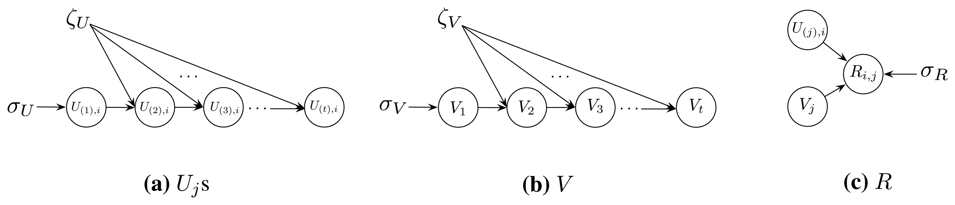
Taking advantage of the knowledge of the probability graph model, we assume that the dependent structure of the data in U(1), U(2), …, U(t), V and R is as illustrated in Figure 1. More specifically, we have the following assumptions:
Columns of U(j) (1 ≤ j ≤ t) are linearly independent, i.e.,
U(1),i (1 ≤ i ≤ n) follows the same Gaussian distribution with a mean of zero and a covariance matrix , i.e.,
U(j),i (1 ≤ i ≤ n) are dependent in time order with the pre-specified priors, ζU and σU, i.e.,
Moreover, for j > 1, we assume U(j),i is a Laplace random vector with location parameter U(j-1),i and scale parameter ζU, namely:
The columns of V are linearly dependent in time order with the pre-specified priors, ζV and σV, i.e.,
We also assume that, for j > 1:
The (i, j)th entry of R (1 ≤ i ≤ n, 1 ≤ j ≤ t) follows Gaussian distribution with a mean of and variance , i.e.,
Now, given R and the priors, σU, σV, σR, ζU, and ζV, let U = {U(1), U(2), …, U(t)}; below, we find a solution to the following equation:
As a supplement, we have the following comments on Model (6):
On the selection of the Gaussian prior: In our model, since no prior information is available for the columns of the matrices, U(1) and V, hence, according to the max entropy principle [26], a reasonable choice for them is the Gaussian prior distribution.
On the ability to formalize the dynamics of the sensor data: The ability to characterize the dynamics of the sensor data lies in the terms and . Obviously, for any two adjacent time points, Tj−1 and Tj, if the interval is small enough (namely, |Tj – Tj−1| → 0), then for any area, Si, the values, Ri,j−1 and Ri,j, should be close to each other (namely, |Ri,j – Ri,j−1| → 0). This can been enforced by tuning the parameters, γ and λ (see the following elaboration).
First of all, since for any x ∈ ℝn, ‖x‖2 ≤ ‖x‖1, we have:
Secondly, it is obvious that greater regularization parameters (i.e., α, β, γ and λ) result in smaller corresponding multipliers (i.e., , , and . In particular:and:Hence, combining Equations (7)-(9), when |Tj – Tj−1| → 0, we can simply take γ → ∞ and λ → ∞ and achieve ‖Rj – Rj−1‖2 → 0.On the other side, when |Tj – Tj−1| → ∞, as is well known, the values in Rj and Rj−1 are regarded as being independent. In this case, we can take γ → 0 and λ → 0, allowing Rj to be irrelevant to Rj−1.
On the ℓ1 norm: It is straightforward to verify that, if we replace the ℓ1 terms in Equation (6) with the ℓ2 terms (equivalently, use the Gaussian distribution instead of the Laplace distribution in Assumptions (III.) and (IV.)), e.g., replacing ‖Vj – Vj−1‖1 with , ‖Rj – Rj−1‖2 can still be bounded via tuning the regularization parameters, γ and λ. The reason for adopting the ℓ1 norm here is two-fold: Firstly, as shown above, the ℓ1 terms can lead to the bounded difference norm, ‖Rj – Rj−1‖2, and hence, the proposed model accommodates the ability to characterize the dynamics of the sensor data; secondly, according to the recent emerging works on compressed sensing [27,28], under some settings, the behavior of the ℓ1 norm is similar to that of the ℓ0 norm. In terms of our model, this result indicates that the ℓ1 terms can restrict not only the magnitudes of the dynamics happening to the features, but also the number of features that changed in adjacent time points. In other words, with ℓ1 norms, our model gains more expressibility.
5. The Algorithm
Below, we present the algorithm to solve Model (6). We denote:
First, we introduce the signum function, sgn, for a real variable, x:
Then, we calculate the partial subgradient of W with regard to U(j),i (1 ≤ i ≤ n and 1 ≤ j ≤ t) as follows:
For j = 2, 3, …, t, define Fj,i,1 = γsgn(U(j),i – U(j−1),i).
For j = 1, 2, …, t – 1, define Fj,i,2 = –γFj+1,i,1.
Let F1,i,1 = Ft,i,2= 0, and we have:
For i = 1, 2 …,n:
For i = 1,2 …,n and j = 2, 3, …, t:
Similarly, we calculate the partial subgradient of W with regard to Vj (1 ≤ j ≤ t):
For 2 ≤ j ≤ t, define Gj,1 = λsgn(Vj – Vj−1).
For 1 ≤ j ≤ t – 1, denote Gj,2 = – Gj+1,1.
Let G1,1 = Gt,2 = 0, and we have:
and for j > 1:
Finally, with the results above, we present the solution algorithm in Algorithm 1.
6. Applications on Missing Sensor Data Imputation
In this section, we evaluate our approach through two large-sized datasets and compare the results with two state-of-the-art algorithms in terms of parametric sensitivity, convergence and missing data recovery performance. The following paragraphs describe the set-up, evaluation methodology and the results obtained. To simplify the parameter tuning, we set α = β and λ = γ in the algorithm implementation.
6.1. Evaluation Methodology
Three state-of-the-art algorithms are selected for comparison to the proposed MMP model. The first one is the k-nearest neighbor-based imputation model [1]. As a local model, for every missing entry, Ri,j, the knnmethod takes the estimation, R̂i,j, as the mean of the k nearest neighbors to it. Let
 (x) be the set consisting of the k non-empty entries to x; then:
The second algorithm is the probabilistic principle components analysis model (PPCA) [30,31], which has achieved state-of-the-art performance in the missing traffic flow data imputation problem [31]. Denote the observations of the incomplete matrix, R, as Ro. Let x ∼ N(0, I); to estimate the missing values, PPCA first fits the parameters μ and C with:
The third algorithm is the probabilistic matrix factorization model (PMF) [7], one of the most popular algorithms targeting the Netflix matrix completion problem. PMF first seeks the low rank matrices, U and V, that:
| Algorithm 1: The Multi-Matrices Factorization Algorithm. | ||
| Input: matrix R; number of the latent features, d; learning rates, η1, η2, η3 and η4; regularization parameters, α and λ; threshold ϵ. | ||
| Output: the estimated matrix, R̂. | ||
| // Initialize U and V. | ||
| 1 | Draw random vectors, U(1),1, U(1),2, …, U(1),n, V1 ∼ N(0, I); | |
| 2 | for j = 2; j ≤ t; j + + do | |
| 3 | Let Vj = Vj−1 + Z; here Z ∼ Laplace(0, 1); | |
| 4 | end | |
| 5 | for j = 2; j ≤ t; j + + do | |
| 6 | for i = 1; i ≤ n; i + + do | |
| 7 | Let U(j),i = U(j-1),i + Z; here Z ∼ Laplace(0, 1); | |
| 8 | end | |
| 9 | end | |
| // Coordinate descent. | ||
| 10 | ; | |
| 11 | ||
| 12 | W2 = inf; | |
| 13 | while |W2 – W1| > ϵ do | |
| 14 | W2 = W1; | |
| 15 | for i= 1, 2 …, n do | |
| 16 | Let ; | |
| 17 | end | |
| 18 | for j > 1 and i = 1, 2 …, n do | |
| 19 | Let | |
| 20 | end | |
| 21 | ; | |
| 22 | for j = 2 …, t do | |
| 23 | Let ; | |
| 24 | end | |
| 25 | Replace all U(j),is with and Vjs with , recompute W1; | |
| 26 | end | |
| 27 | return R̂, where ; | |
These three algorithms, as well as the proposed MMF, are employed to perform missing imputations for the incomplete matrix, R, on the same datasets.
The testing protocol adopted here is the Given X (0 < X < 1) protocol [32], i.e., given a matrix, R, only X percent of its observed entries are revealed, while the remaining observations are concealed to evaluate the trained model. For example, a setting with X = 10% means that the algorithm is trained with 10% of the non-missing entries, and the rest of the 90% non-missing ones are held and are to be recovered. In both of the experiments on synthetic and real datasets, the data partition is repeated five times, and the average results, as well as the standard deviations over the five repetitions are recorded.
Similar to many other missing imputation problems [1,3-5,7,13,33-35], we employ the root mean square error (RMSE) to depict the distance between the real values and the estimations: Let S = {s1, s2, … sn} be the test dataset and Ŝ = {ŝ1, ŝ2, … ŝn} be the estimated set; here, ŝi is the estimation of si. Then, the RMSE of the estimation is given by .
6.2. Synthetic Validation
To conduct a synthetic validation of the studied approaches, we randomly draw a 100 × 10, 000 matrix R using the procedure detailed in Algorithm 2. The rows in R correspond to the areas, S1, S2, …, Sn, and the columns correspond to the time. Thus, Ri,j represents the data collected in Si at time Tj. Notably, the parameter, ri,j, in Algorithm 2 is used to control the magnitude of the variation happening to Si from Tj−1 to Tj. Combining lines 4 and 5, we have: for i ∈ [1, n] and j ∈ [1, t], . This constraint ensures that the data collected in Si does not change too much over time Tj−1 to Tj.
| Algorithm 2: Synthetic Data Generating Procedure. | |
| 1 | for i = 1, 2, …, n do |
| 2 | Draw Ri,1 ∼ N(0, 1); |
| 3 | for j = 2, 3, …, t do |
| 4 | Let ri,j ∼ Uniform(−0.1, 0.1); |
| 5 | Ri,j ← Ri,j−1 + ri,jRi,j−1; |
| 6 | end |
| 7 | end |
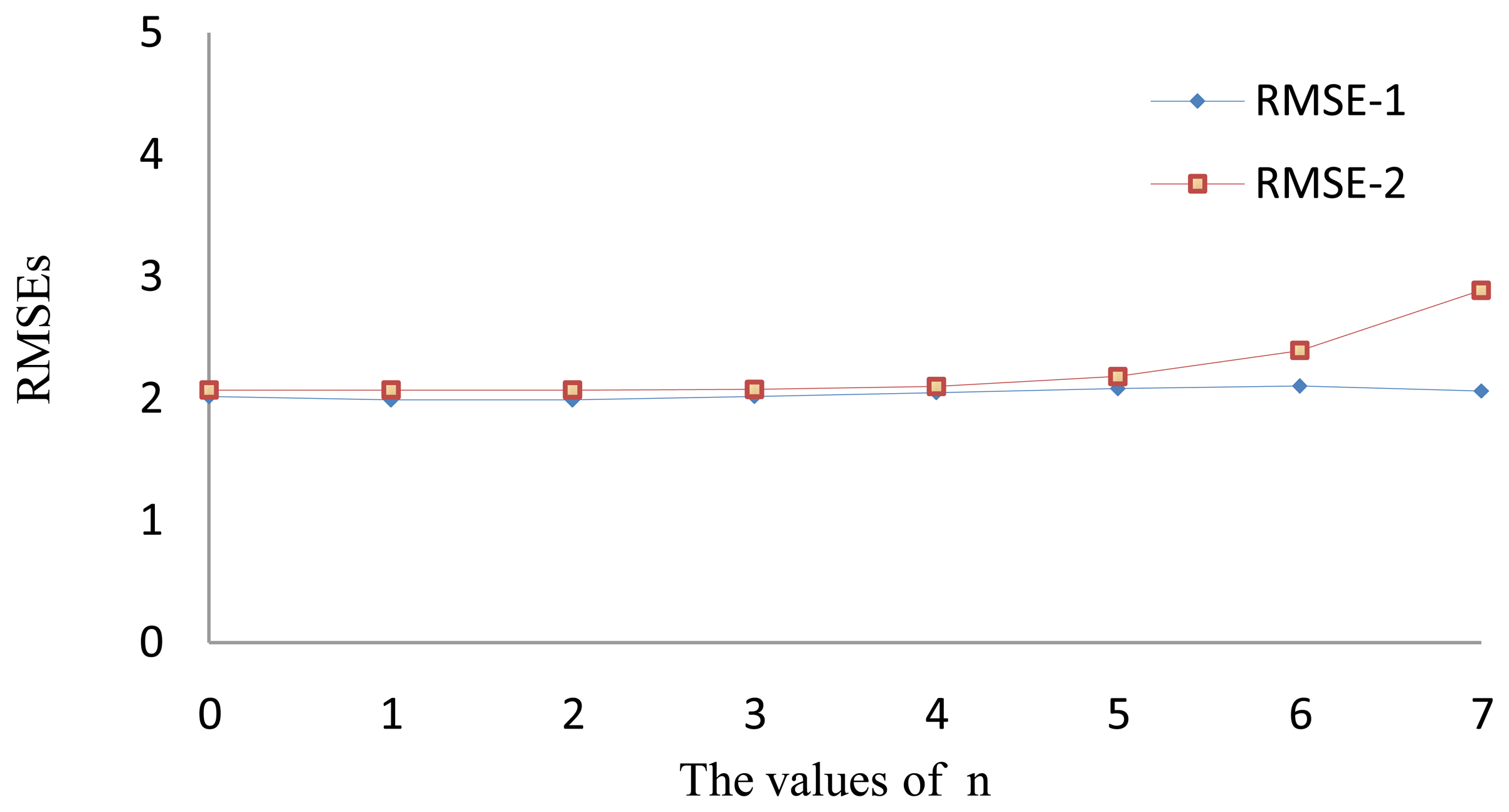
We first evaluate the sensitivity of the proposed algorithm to the regularization parameters, α and λ. Half of the entries in R are randomly selected as testing data and recovered using the remaining 50% as the training data. Namely, we take X = 50% in the Given X protocol. In the experiments, we first fix α = 0.01, tune λ via λ = 0.01 × 2n (n = 0, 1, … 7) and, then, do the reverse by changing α via α = 0.01 × 2n (n = 0, 1, … 7), but setting λ = 0.01. The average RMSEs with the same parameter settings on different data partitions are summarized in Figure 2.
In Figure 2, the RMSE-1 curve represents the recovery errors obtained by fixing α and changing the value of λ. The RMSE-2 curve corresponds to the errors with different α values and fixed λ. We can see that even when λ is expanded by more than 100 times (27 = 128), the RMSE still remains stable. A similar result also appears in the experiments on the parameter, α, where a significant change of the RMSE only occurs when n is greater than six, i.e., when α is expanded more than 60 times.
The second experiment we conduct is to study the prediction ability of the proposed algorithm, as well as that of the comparison algorithms. In the Given X protocol, we set X = 10%, 20%, …, 90% in sequence. Then, for each X value, we perform missing imputations via our algorithm and the comparison algorithms. In the all implementations, we set k = 5 for the knn model. As with the MF-based algorithms, we examine their performance with respect to the latent feature dimension d = 10 and d = 30 respectively. Furthermore, in the implementation of MMF, we fix α = λ = 0.1, η1 = η2 = η3 = η4 = 0.01. All results are summarized in Table 1.
As shown in Table 1, when X is large, e.g., X ≥ 50%, knn is competitive with the matrix factorization methods, while in the other situations, the MF methods outperform it significantly. In terms of the MF-based methods, we find that our algorithm outperforms PPCA significantly in all settings. The RMSEs of our algorithm are at most roughly 20% of that of PPCA. Specifically, for X ∈ [30%; 80%], the RMSEs of the proposed algorithm are even only 10% of that of PPCA. We can also observe that the parameter, d, has a different impact on the performances of our algorithm and PPCA: When d changes from 10 to 30, most of the RMSEs of PPCA increase evidently, while for our algorithm, the RMSEs are reduced by roughly 5%.
When compared with PMF, our algorithm also performs better in most of the settings: PMF achieves lower RMSEs than MMF only in two cases, in which d = 10, X = 60% and d = 10; X = 80% respectively. Another interesting finding is that the promotion of the feature number, d (from 10 to 30), has little impact on the performance of PMF.
We also exam the convergence speed of the proposed algorithm. In the missing recovery experiments conducted above, for each X setting, we record the average RMSE of the recovered results after every 10 iterations of all data partitions. We can see from Figure 3 that, for all X values, the errors drop dramatically in the first 20 iterations and remain stable after the first 100 iterations. We can conclude that the proposed algorithm converges to the local optimization solutions after around 100 iterations.
6.3. Application to Impute the Missing Traffic Speed Values
To evaluate the feasibility of the proposed approach on real-world applications, in this section, we conduct another experiment on a traffic speed dataset, which was collected in the urban road network of Zhuhai City [36], China, from April 1, 2011 to April 30, 2011. The data matrix, R, consists of 1,853 rows and 8,729 columns. Each row corresponds to a road, and each column corresponds to a five minute-length time interval. All columns are arranged in ascending order of time. An entry, Ri,j (1 ≤ i ≤ 1, 853,1 ≤ j ≤ 8729), in R is the aggregate mean traffic speed of the ith road in the jth interval. Since all the data in R are collected by floating cars [37], the value of Ri,j could be missing if there is no car on the i th road in the j th time interval. Our statistics show that in R, there are nearly half of the entries, i.e., eight million entries are missing values.
We perform missing imputation on matrix R using the studied algorithms with parameter settings k = 5 and d = 10. In the implementation of MMF, we fix α = 0.25, λ = 0.5, η1 = η2 = η3 = η4 = 0.5. We summarize all results in Table 2, from which both the feasibility and effectiveness of MMF are well verified. In detail, when X is large enough, e.g., X ≥ 80%, knn is competitive, while in the other cases, knn cannot work as well as the MF based algorithms. As for the MF algorithms, we see that the proposed MMF outperforms PPCA and PMF in all X settings. Particularly, when the observations are few (X = 10% and X = 20%), the errors of our algorithm reduce by 33% compared to those of PPCA and by 10% compared to those of PMF, respectively. When X > 20%, the RMSE differences between PPCA and our algorithm tend to be slight, but the overall errors of PPCA are roughly 3% ∼ 5% higher than those of MMF. For PMF, the RMSEs remain about 10% higher than MMF in all settings.
7. Conclusion
Missing estimation is one of the main concerns in current studies on sensor data-based applications. In this work, we formulate the estimation problem as a matrix completion one and present a multi-matrices factorization model to address it. In our model, each column, Rj, of the target matrix, R, is approximated by the product of a spatial feature matrix, U(j), and a temporal feature vector, Vj. Both Uj and Vj are time dependent, and hence, their product accommodates the ability to describe the time variant sensor data. We also present a solution algorithm to the factorization model. Empirical studies on a synthetic dataset and real sensor data show that our approach outperforms the comparison algorithms.
Reviewing the present work, it is notable that the proposed model only incorporates the temporal structure information, while the information on the spatial structure is disregarded, e.g., the data collected in two adjacent areas, Sk and Sl, should be close to each other. Hence, our next step is to extend our model with more complex structured data.
Acknowledgments
This work has been partially supported by National High-tech R&D Program (863 Program) of China under Grant 2012AA12A203.
Conflicts of Interest
The authors declare no conflict of interest.
References
- García-Laencina, P.J.; Sancho-Gómez, J.L.; Figueiras-Vidal, A.R.; Verleysen, M. K nearest neighbours with mutual information for simultaneous classification and missing data imputation. Neurocomputation 2009, 72, 1483–1493. [Google Scholar]
- Ni, D.; Leonard, J.D.; Guin, A.; Feng, C. Multiple imputation scheme for overcoming the missing values and variability issues in ITS data. J. Transport. Eng. 2005, 131, 931–938. [Google Scholar]
- Smith, B.L.; Scherer, W.T.; Conklin, J.H. Exploring imputation techniques for missing data in transportation management systems. Transport. Res. Record. J. Transport. Res. Board 2003, 1836, 132–142. [Google Scholar]
- Qu, L.; Zhang, Y.; Hu, J.; Jia, L.; Li, L. A BPCA Based Missing Value Imputing Method for Traffic Flow Volume Data. Proceedings of 2008 IEEE Intelligent Vehicles Symposium, Eindhoven, The Neatherlands, 4–6 June 2008; pp. 985–990.
- Jiang, N.; Gruenwald, L. Estimating Missing Data in Data Streams. In Advances in Databases: Concepts, Systems and Applications; Springer: Berlin/Heidelberg, Germany, 2007; pp. 981–987. [Google Scholar]
- Netflix Prize. Avaiable online: http://www.netflixprize.com (accessed on 1 July 2013).
- Salakhutdinov, R.; Mnih, A. Probabilistic matrix factorization. Adv. Neural Inf. Process. Syst. 2008, 20, 1257–1264. [Google Scholar]
- Koren, Y. Factorization Meets the Neighborhood: A Multifaceted Collaborative Filtering Model. Proceedings of the 14th ACM SIGKDD International Conference on Knowledge Discovery and Data Mining, Las Vegas, NV, USA; 2008; pp. 426–434. [Google Scholar]
- Seung, D.; Lee, L. Algorithms for non-negative matrix factorization. Adv. Neural Inf. Process. Syst. 2001, 13, 556–562. [Google Scholar]
- Srebro, N. Learning with Matrix Factorizations. Ph.D Thesis, Department of Electrical Engineering and Computer Science, Massachusetts Institute of Technology, Cambridge, MA, USA, 2004. [Google Scholar]
- Srebro, N.; Rennie, J.D.; Jaakkola, T. Maximum-margin matrix factorization. Adv. Neural Inf. Process. Syst. 2005, 17, 1329–1336. [Google Scholar]
- Independent and identically distributed random variables. Avaiable online: http://en.wikipedia.org/wiki/ndependent_and_identically_distributed_random_variables (accessed on 1 July 2013).
- Koren, Y.; Bell, R.; Volinsky, C. Matrix factorization techniques for rcommender systems. Computer 2009, 42, 30–37. [Google Scholar]
- Xu, W.; Liu, X.; Gong, Y. Document Clustering Based on Non-Negative Matrix Factorization. Proceedings of the 26th Annual International ACM SIGIR Conference on Research and Development in Informaion Retrieval, Pisa, Italy, 28 July–1 August 2003; pp. 267–273.
- Lee, D.D.; Seung, H.S. Learning the parts of objects by non-negative matrix factorization. Nature 1999, 401, 788–791. [Google Scholar]
- Brunet, J.P.; Tamayo, P.; Golub, T.R.; Mesirov, J.P. Metagenes and molecular pattern discovery using matrix factorization. Proc. Natl. Acad. Sci. USA 2004, 101, 4164–4169. [Google Scholar]
- Candès, E.J.; Recht, B. Exact matrix completion via convex optimization. Found. Comput. Math. 2009, 9, 717–772. [Google Scholar]
- Hoyer, P.O. Non-negative matrix factorization with sparseness constraints. J. Mach. Learn. Res. 2004, 5, 1457–1469. [Google Scholar]
- Mairal, J.; Bach, F.; Ponce, J.; Sapiro, G. Online learning for matrix factorization and sparse coding. J. Mach. Learn. Res. 2010, 11, 19–60. [Google Scholar]
- Ke, Q.; Kanade, T. Robust L1Norm Factorization in the Presence of Outliers and Missing Data by Alternative Convex Programming. Proceedings of the 2005 IEEE Computer Society Conference on Computer Vision and Pattern Recognition (CVPR 2005), San Diego, CA, USA, 20–26 June 2005; pp. 739–746.
- Nati, N.S.; Jaakkola, T. Weighted Low-Rank Approximations. proceedings of the 20th International Conference on Machine Learning (ICML 2003), Washington, DC, USA, 21–24 August 2003; pp. 720–727.
- Abernethy, J.; Bach, F.; Evgeniou, T.; Vert, J.P. Low-Rank Matrix Factorization with Attributes; Technical Report; N-24/06/MM; Paris, France; September; 2006. [Google Scholar]
- Vapnik, V. Statistical Learning Theory; Wiley: New York, NY, USA, 1998. [Google Scholar]
- Rissanen, J. Minimum Description Length Principle; Springer: Berlin, Germany, 2010. [Google Scholar]
- Candè s, E.J.; Tao, T. The power of convex relaxation: Near-optimal matrix completion. IEEE Trans. Inf. Theory 2010, 56, 2053–2080. [Google Scholar]
- Cover, T.M.; Thomas, J.A. Elements of Information Theory; John Wiley & Sons: Hoboken, NJ, USA, 2012. [Google Scholar]
- Candès, E.J.; Romberg, J.; Tao, T. Robust uncertainty principles: Exact signal reconstruction from highly incomplete frequencyinformation. IEEE Trans. Inf. Theory 2006, 52, 489–509. [Google Scholar]
- Donoho, D.L. Compressed sensing. IEEE Trans. Inf. Theory 2006, 52, 1289–1306. [Google Scholar]
- Bertsekas, D.P. Nonlinear Programming; Athena Scientific: Belmont, MA, USA, 1999. [Google Scholar]
- Tipping, M.E.; Bishop, C.M. Probabilistic principal component analysis. J. Royal Stat. Soc. Ser. B Stat. Methodol. 1999, 61, 611–622. [Google Scholar]
- Qu, L.; Hu, J.; Li, L.; Zhang, Y. PPCA-based missing data imputation for traffic flow volume: A systematical approach. IEEE Trans. Intell. Transport. Syst. 2009, 10, 512–522. [Google Scholar]
- Marlin, B. Collaborative Filtering: A Machine Learning Perspective. Ph.D Thesis, University of Toronto, ON, Canada, 2004. [Google Scholar]
- Nguyen, L.N.; Scherer, W.T. Imputation Techniques to Account for Missing Data in Support of Intelligent Transportation Systems Applications; UVACTS-13-0-78; University of Virginia: Charlottesville: Charlottesville, VA, USA, 2003. [Google Scholar]
- Gold, D.L.; Turner, S.M.; Gajewski, B.J.; Spiegelman, C. Imputing Missing Values in Its Data Archives for Intervals under 5 Minutes. Proceedings of 80th Annual Meeting of Transportation Research Board, Washington, DC, USA, 7–11 January 2001.
- Shuai, M.; Xie, K.; Pu, W.; Song, G.; Ma, X. An Online Approach Based on Locally Weighted Learning for Real Time Traffic Flow Prediction. The 16th ACM SIGSPATIAL International Conference on Advances in Geographic Information Systems (ACM GIS 2008), Irvine, CA, USA, 5–7 November 2008.
- Zhuhai. Avaiable online: http://en.wikipedia.org/wiki/Zhuhai (accessed on 1 July 2013).
- Floating Car Data. Avaiable online: http://en.wikipedia.org/wiki/Floating_car_data (accessed on 1 July 2013).


| 10% | 20% | 30% | 40% | 50% | 60% | 70% | 80% | 90% | ||
|---|---|---|---|---|---|---|---|---|---|---|
| knn | 13.41 ± 0.62 | 6.80 ± 0.19 | 4.44 ± 0.06 | 3.12 ± 0.05 | 2.27 ± 0.02 | 1.81 ± 0.09 | 1.72 ± 0.01 | 1.69 ± 0.05 | 1.62 ± 0.06 | |
| d = 10 | PPCA | 17.09 ± 2.08 | 20.24 ± 1.30 | 22.75 ± 1.32 | 23.96 ± 2.19 | 20.79 ± 1.00 | 16.67 ± 1.34 | 18.68 ± 0.81 | 11.98 ± 0.70 | 5.11 ± 3.10 |
| PMF | 3.23 ± 0.23 | 3.33 ± 0.19 | 3.29 ± 0.12 | 3.34 ± 0.07 | 3.29 ± 0.09 | 1.69 ± 0.04 | 1.83 ± 0.02 | 1.81 ± 0.03 | 1.85 ± 0.04 | |
| MMF | 3.07 ± 0.07 | 2.21 ± 0.10 | 2.14 ± 0.09 | 1.98 ± 0.06 | 1.93 ± 0.06 | 1.92 ± 0.04 | 1.75 ± 0.03 | 1.84 ± 0.02 | 1.80 ± 0.03 | |
| d = 30 | PPCA | 19.65±3.01 | 22.48 ± 0.86 | 24.86 ± 1.54 | 23.99 ± 0.61 | 22.67 ± 0.49 | 20.22 ± 1.46 | 17.53 ± 0.70 | 14.23 ± 1.70 | 11.14 ± 1.72 |
| PMF | 3.20 ± 0.21 | 3.32 ± 0.13 | 3.35 ± 0.09 | 3.36 ± 0.11 | 3.31 ± 0.07 | 1.78 ± 0.04 | 1.81 ± 0.02 | 1.79 ± 0.02 | 1.86 ± 0.11 | |
| MMF | 3.06 ± 0.05 | 2.17 ± 0.08 | 2.07 ± 0.05 | 1.94 ± 0.03 | 1.74 ± 0.03 | 1.62 ± 0.02 | 1.64 ± 0.03 | 1.65 ± 0.01 | 1.69 ± 0.03 | |
| 10% | 20% | 30% | 40% | 50% | 60% | 70% | 80% | 90% | |
|---|---|---|---|---|---|---|---|---|---|
| knn | 40.47 ± 0.02 | 31.79 ± 0.01 | 25.41 ± 0.02 | 21.35 ± 0.00 | 18.33 ± 0.00 | 15.89 ± 0.01 | 13.73 ± 0.01 | 11.67 ± 0.00 | 9.45 ± 0.02 |
| PPCA | 17.90 ± 0.01 | 17.36 ± 0.01 | 13.00 ± 0.02 | 12.25 ± 0.01 | 11.47 ± 0.01 | 11.31 ± 0.03 | 11.19 ± 0.02 | 11.14 ± 0.04 | 11.16 ± 0.10 |
| PMF | 14.41 ± 0.01 | 12.83 ± 0.03 | 12.43 ± 0.01 | 12.33 ± 0.02 | 12.36 ± 0.01 | 12.35 ± 0.01 | 12.13 ± 0.00 | 11.99 ± 0.03 | 11.96 ± 0.02 |
| MMF | 11.79 ± 0.02 | 11.51 ± 0.01 | 11.43 ± 0.01 | 11.05 ± 0.02 | 11.05 ± 0.01 | 11.01 ± 0.00 | 10.83 ± 0.01 | 10.69 ± 0.01 | 10.70 ± 0.02 |
© 2013 by the authors; licensee MDPI, Basel, Switzerland. This article is an open access article distributed under the terms and conditions of the Creative Commons Attribution license (http://creativecommons.org/licenses/by/3.0/).
Share and Cite
Huang, X.-Y.; Li, W.; Chen, K.; Xiang, X.-H.; Pan, R.; Li, L.; Cai, W.-X. Multi-Matrices Factorization with Application to Missing Sensor Data Imputation. Sensors 2013, 13, 15172-15186. https://doi.org/10.3390/s131115172
Huang X-Y, Li W, Chen K, Xiang X-H, Pan R, Li L, Cai W-X. Multi-Matrices Factorization with Application to Missing Sensor Data Imputation. Sensors. 2013; 13(11):15172-15186. https://doi.org/10.3390/s131115172
Chicago/Turabian StyleHuang, Xiao-Yu, Wubin Li, Kang Chen, Xian-Hong Xiang, Rong Pan, Lei Li, and Wen-Xue Cai. 2013. "Multi-Matrices Factorization with Application to Missing Sensor Data Imputation" Sensors 13, no. 11: 15172-15186. https://doi.org/10.3390/s131115172