Dynamic Strain Measured by Mach-Zehnder Interferometric Optical Fiber Sensors

Abstract
: Optical fibers possess many advantages such as small size, light weight and immunity to electro-magnetic interference that meet the sensing requirements to a large extent. In this investigation, a Mach-Zehnder interferometric optical fiber sensor is used to measure the dynamic strain of a vibrating cantilever beam. A 3 × 3 coupler is employed to demodulate the phase shift of the Mach-Zehnder interferometer. The dynamic strain of a cantilever beam subjected to base excitation is determined by the optical fiber sensor. The experimental results are validated with the strain gauge.1. Introduction
Optical fiber sensors have attracted considerable attention in recent years as powerful measurement devices. They have been used in a variety of engineering applications such as residual strain measurement in composites [1], thin film stress measurement [2], monitoring mixed mode cracks [3], and gas detection [4]. Due to their small size and light weight, optical fiber sensors are appropriate for embedding or surface bonding to the structures. Optical fiber sensors can be classified according to the light parameters that are modulated. They are three types of sensors: the intensity, the phase and the wavelength modulated [5].
Vibrations have a significant effect on the fatigue life of structures and may even have disastrous consequences. To understand the vibrating behavior of structures, instrumentation for accurate vibration measurement is essential. A number of sensors are available for the measurements of a vibrating structure including strain gauge, piezoelectric transducer, laser vibrometer, accelerometer and optical fiber sensor. Among these measurement devices, optical fiber sensors have received much attention for structural health monitoring applications. They are unique in a number of aspects including small physical size, ease of embedment in structures, immunity to electromagnetic interference and excellent multiplexing capabilities [6], which make them ideal for vibration measurement. The fiber Bragg grating (FBG) and extrinsic Fabry-Perot interferometer (EFPI) techniques have been successfully demonstrated for the measurement of structural dynamic responses. Jin et al. [7] used fibre-optic grating sensors for flow induced vibration measurement. Betz et al. [8] developed a damage localization and detection system based on fiber Bragg grating Rosettes and lamb waves. Kirkby et al. [9] demonstrated the localization of impact in carbon fiber reinforced composites using a sparse array of FBG sensors. Frieden et al. [10,11] presented a method for the localization of an impact and identification of an eventual damage using dynamic strain signals from fiber Bragg grating (FBG) sensors. EFPI sensors have been used for strain measurement [12,13] and acoustic emission [5,14,15]. The EFPI sensor is more sensitive than the FBG, but the demodulation required high cost methodologies.
In this work, Mach-Zehnder optical fiber interferometric sensor is employed to measure the dynamic strain of a vibrating cantilever beam. The method developed by Brown et al. [16,17] for demodulation of the phase shift is adopted. The demodulation scheme utilizes a 3 × 3 coupler to reconstruct the signal of interest. The demodulation scheme has the advantage of passive detection and low cost as it requires no phase or frequency modulation in reference arm [18]. The experimental test results are validated with the strain gauge.
2. Mach-Zehnder Interferometer
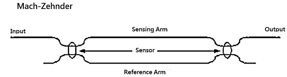
The schematic diagram of a Mach-Zehnder interferometer is shown in Figure 1. It consists of two 2 × 2 couplers at the input and output. The excitation is applied to the sensing fiber, resulting optical path difference between the reference and sensing fibers. The light intensity of the output of the Mach-Zehnder interferometer can be expressed as [19]:
The integral of the strain in Equation (2) denotes the change of the length of the sensing fiber which is surface bonded onto the host structure. The average strain of the optical fiber for optical phase shift Δϕ is:
Thus, once the phase shift Δϕ of the Mach-Zehnder interferometer is demodulated, the strain of the host structure can be determined by utilizing Equation (3).
3. Demodulation of Phase Shift
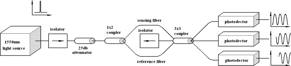
To demodulate phase shift Δϕ of the Mach-Zehnder interferometer, a 3 × 3 coupler is employed. Figure 2 shows the schematic diagram of the demodulation scheme. It consists of a 1 × 2 coupler at the input and a 3 × 3 coupler at the output. The two outputs of the 1 × 2 coupler comprise the reference fiber and sensing fiber of the Mach-Zehnder interferometer. The sensing fiber is surface bonded onto the host structure. Mechanical or thermal loadings applied to the host structure, leads to an optical path difference between the two fibers. The difference in the optical path induces a relative phase shift in the Mach-Zehnder interferometer. The two optical signals are guided into two of the three inputs of a 3 × 3 coupler, where they interfere with one another. The methodology developed by Brown et al. [16,17] for demodulation of the phase shift is adopted and briefly described as follows.
The three outputs of the 3 × 3 coupler are nominally 120° out of phase with either of its neighbors and can be expressed as:
The DC offset “C” of the output can be obtained by adding the three inputs as follows:
Three new parameters, y1, y2 and y3 are introduced as follows:
The next step in the processing is to take the difference between each of the three possible pairings of the derivatives (ẏ, ẏ2, ẏ3) and multiply this by the third signal (not differentiated):
Summation of Equations (7a), (7b) and (7c), yields:
Taking the squares of Equations (6a), (6b) and (6c), then adding them, leads to:
Dividing Equation (9) into Equation (8), yields:
We can integrate Equation (10) to obtain the phase shift Δϕ(t) as follows:
Thus, the strain in the host structure is readily to be determined by substituting phase shift Δϕ(t) from Equation (11) into Equation (3).
In this study, the phase shift demodulation is performed using the commercial software Matlab. Figure 3 shows the block diagram of the demodulation process.
4. Numerical Example
To demonstrate the capability of the proposed methodology in demodulating the phase shift, a numerical example is presented. In the numerical example, the phase shift is assumed to be a sinusoidal function with dual angular frequencies of 34π and 50π as follows:
Substituting Equation (12) into Equations (4a), (4b) and (4c) leads to the three outputs of the 3 × 3 coupler:
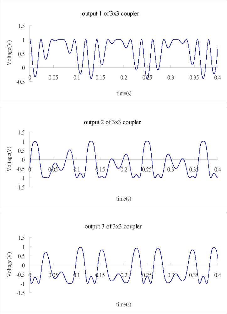
Figure 4 shows the three outputs of the 3 × 3 coupler where C and B are taken to be 0 and 1, respectively.
Substituting the numerical data of the three outputs from Figure 4 into Matlab software, follows the process as shown in the block diagram of Figure 3 to demodulate the phase shift. Figure 5 illustrates the results of phase shift demodulated by Matlab, and compares with the exact phase shift Equation (12). It appears that the demodulated phase shift is almost the same as the exact phase shift.
5. Experimental Tests
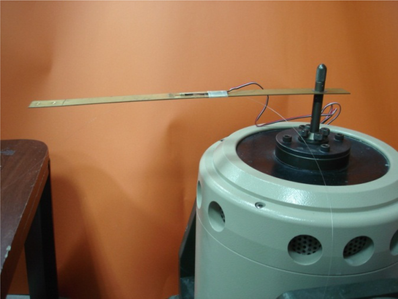
A cantilever beam subjected to base excitation is considered in the experimental test. The beam of length L = 285 mm, width b = 20 mm, thickness h = 1 mm is made of copper with elastic modulus E = 120 GPa, density ρ = 8,740 kg/m3. An optical fiber is surface bonded to the middle of the cantilever beam as the sensing fiber of the Mach-Zehnder interferometer. The percentage of the strain in the test specimen actually transferred to the optical fiber is dependent on the bonding length [20]. The bonding length is Lf = 60 mm in this work. The material properties for the optical fiber are [21]: elastic modulus Ef = 72 GPa, Poisson’s ratio vf = 0.17, index of refraction n0 = 1.45, pockel’s constants p11 = 0.12, p12 = 0.27, radius rf = 62.5 μm. An electric resistance strain gauge is adhered to the cantilever beam near by the optical fiber. The optical fiber sensing system is a Mach-Zehnder interferometer with a 3 × 3 coupler as shown in Figure 2, operating at the wavelength of λ = 1,547.28 nm. The cantilever beam is mounted on a shaker as shown in Figure 6. The shaker is capable of providing maximum of four different frequencies in the same test. The natural frequency of a cantilever beam can be calculated using the following equations:
The first five natural frequencies for the testing cantilever beam are 7.37 Hz, 46.21 Hz, 129.39 Hz, 253.63 Hz and 419.23 Hz, respectively. In the experimental test, the cantilever beam is excited by a shaker with different frequencies.
5.1. Test Case 1
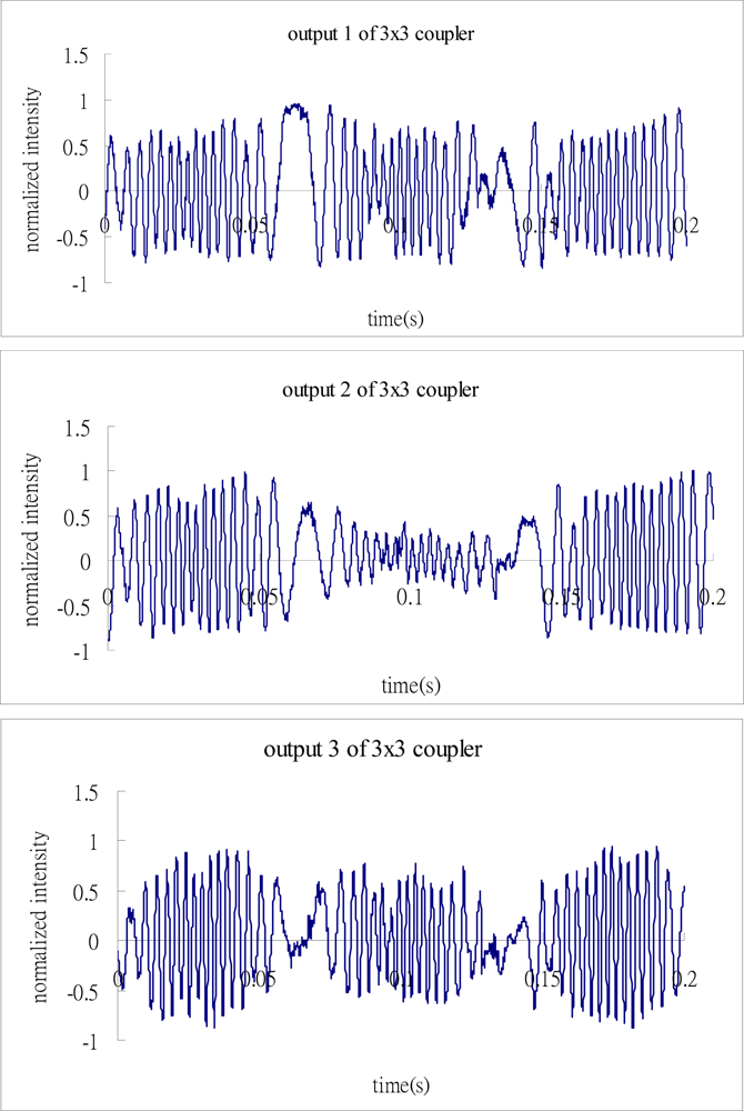
The cantilever beam is excited by a shaker with the frequency of 7 Hz which is approximate to the first natural frequency of 7.37 Hz. Figure 7 shows the signals of the three outputs of the 3 × 3 coupler.
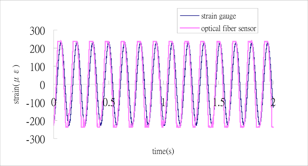
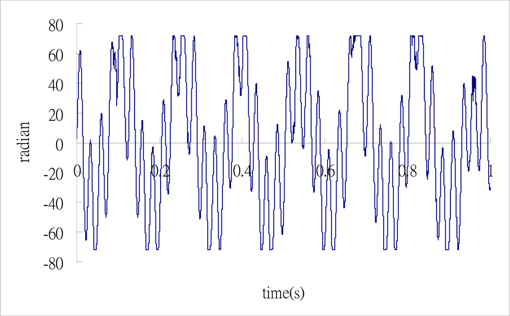
Substituting the three output signals of the 3 × 3 coupler as shown in Figure 7 into the Matlab software, performs the phase shift demodulation as shown in Figure 3. The result of the demodulated phase shift is presented in Figure 8. Substituting the phase shift Δϕ(t) from Figure 8 into Equation (3), leads to the determination of the dynamic strain of the cantilever beam. The dynamic strains obtained by the optical fiber sensor are compared with the results of the strain gauge as shown in Figure 9. Good agreement is achieved between these two sensors.
5.2. Test Case 2
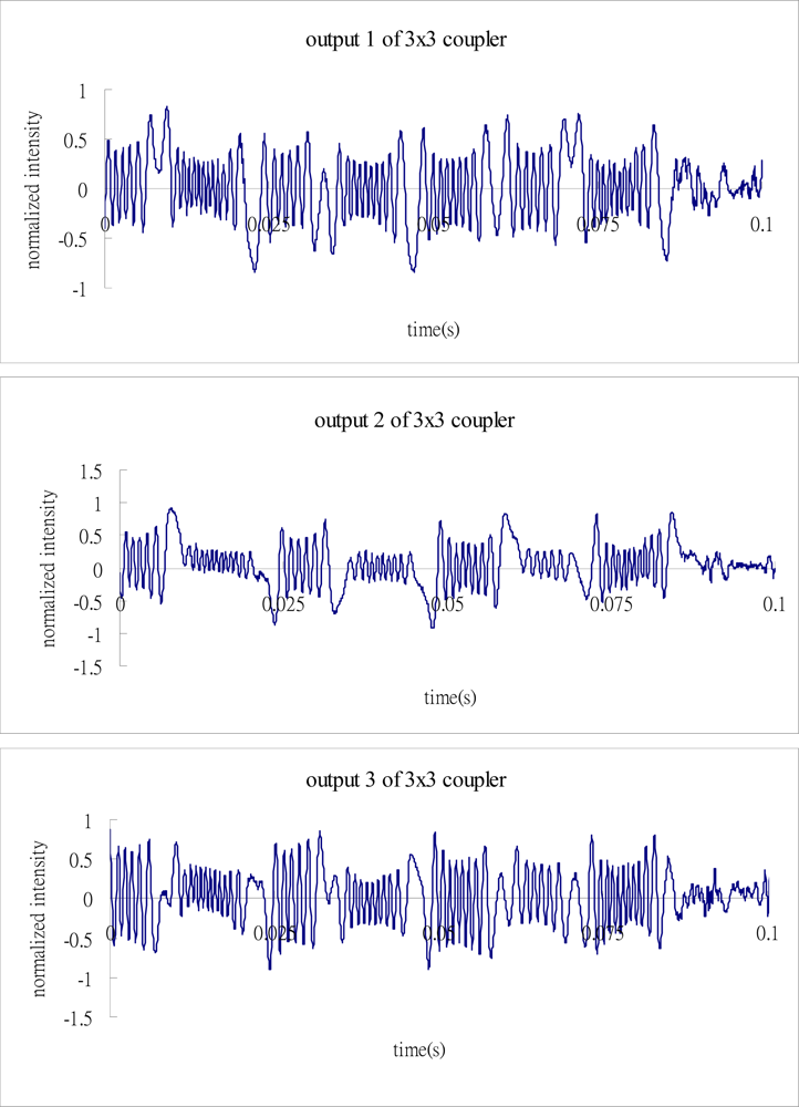
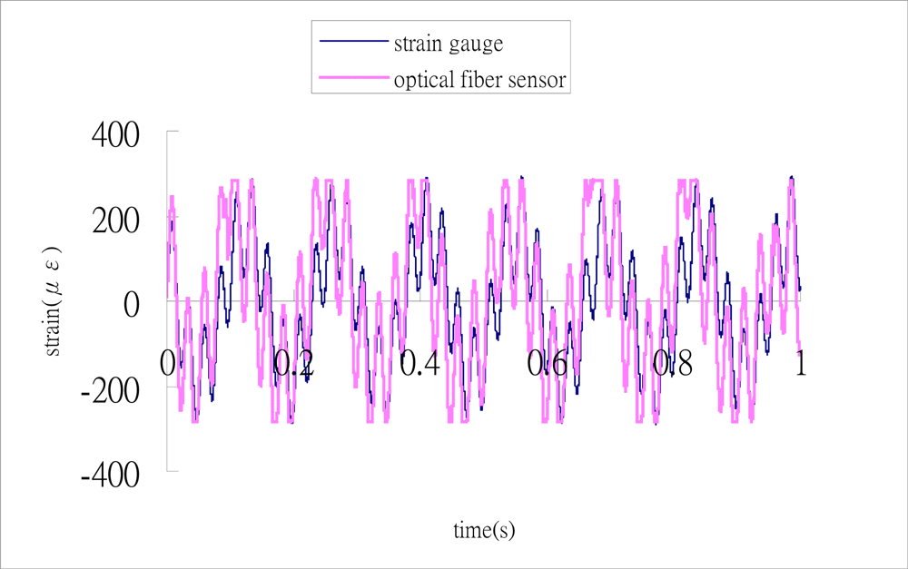
The cantilever beam is excited by the shaker with dual frequencies of 7 Hz and 40 Hz, respectively. The three output signals from the 3 × 3 coupler are plotted in Figure 10.
Substituting these three output signals of the 3 × 3 coupler as shown in Figure 10 into Matlab software, conducts the phase shift demodulation. The result of the phase shift is illustrated in Figure 11. Substituting the phase shift Δϕ(t) from Figure 11 into Equation (3), leads to the dynamic strain of the cantilever beam. The dynamic strains obtained by the optical fiber sensor are compared with the results of the strain gauge as shown in Figure 12. Reasonable agreement is observed between these two sensors. The difference of dynamics strains measured by the optical fiber sensor and strain gauge shown in Figure 12 is about 10 %. The discrepancy can be attributed to the noise of the signals.
6. Conclusions
Optical fiber sensors have been demonstrated for their capability to measure the dynamic responses of structures. They permit continuous monitoring of the integrity of the host structures. An optical fiber system has been developed for dynamic sensing in real time. This was done using a Mach-Zehnder interferometer incorporated with a 3 × 3 coupler for strain sensing under dynamic loading. In this work, the phase shift demodulation of the Mach-Zehnder interferometer is carried out using the commercial software Matlab. In the experimental test, the dynamic response measured by the optical fiber sensor for a cantilever beam subjected to base excitation is validated with the result of strain gauge. There is no particular restriction on the frequency of the vibrating structures in the proposed model. However, to measure the high frequency responses, it requires a data acquisition system with high sampling rate. The proposed optical fiber system is simple, inexpensive and easy to implement; moreover, it is high sensitive and accurate. These superior characteristics make it very useful and attractive for dynamic sensing.
Acknowledgments
The authors gratefully acknowledge the financial support provided by National Science Council of ROC under Grant No. NSC 99-2221-E-155-012 for this work.
References and Notes
- Sorensen, L.; Gmur, T.; Botsis, J. Residual strain development in an AS4/PPS thermoplastic composite measured using fibre Bragg grating sensors. Composites Part A 2006, 37, 270–281. [Google Scholar]
- Quintero, S.M.M.; Quirino, W.G.; Triques, A.L.C.; Valente, L.C.G.; Braga, A.M.B.; Achete, C.A.; Cremona, M. Thin film stress measurement by fiber optic strain gage. Thin Solid Films 2006, 494, 141–145. [Google Scholar]
- Wan, K.T.; Leung, C.K.Y. Fiber optic sensor for the monitoring of mixed mode cracks in structures. Sens. Actuat. A 2007, 135, 370–380. [Google Scholar]
- Benounis, M.; Aka-Ngnui, T.; Jaffrezic, N.; Dutasta, J.P. NIR and optical fiber sensor for gases detection produced by transformation oil degradation. Sens. Actuat. A 2008, 141, 76–83. [Google Scholar]
- de Oliveira, R.; Ramos, C.A.; Marques, A.T. Health monitoring of composite structures by embedded FBG and interferometric Fabry-Perot sensors. Comput. Struct 2008, 86, 340–346. [Google Scholar]
- Li, H.C.H; Herszberg, I.; Davis, C.E.; Mouritz, A.P.; Galea, S.C. Health monitoring of marine composite structural joints using fibre optic sensors. Comput. Struct 2006, 75, 321–327. [Google Scholar]
- Jin, W.; Zhou, Y.; Chan, P.K.C.; Xu, H.G. A fibre-optic grating sensor for the study of flow-induced vibrations. Sens. Actuat. A 2000, 79, 36–45. [Google Scholar]
- Betz, D.C.; Thursby, G.; Culshaw, B.; Staszewski, W.J. Structural damage location with fiber Bragg grating rosettes and lamb waves. Struct. Health Monit 2007, 6, 299–308. [Google Scholar]
- Kirkby, E.; de Oliveira, R.; Michaud, V.; Manson, J.A. Impact localisation with FBG for a self-healing carbon fibre composite structure. Composite Struct 2011, 94, 8–14. [Google Scholar]
- Frieden, J.; Cugnoni, J.; Botsis, J.; Gmur, T. Low energy impact damage monitoring of composites using dynamic strain signals from FBG sensors—Part I: Impact detection and localization. Composite Struct 2012, 94, 438–445. [Google Scholar]
- Frieden, J.; Cugnoni, J.; Botsis, J.; Gmur, T. Low energy impact damage monitoring of composites using dynamic strain signals from FBG sensors—Part II: Damage identification. Composite Struct 2012, 94, 593–600. [Google Scholar]
- Liu, T.; Wu, M.; Rao, Y.; Jackson, D.A.; Fernando, G.F. A multiplexed optical fibre-based extrinsic Fabry-Perot sensor system for in situ strain monitoring in composites. Smart Mater. Struct 1998, 7, 550–556. [Google Scholar]
- Zhou, G.; Sim, L.M.; Loughlan, J. Damage evaluation of smart composite beams using embedded extrinsic Fabry-Perot interferometric strain sensors: Bending stiffness assessment. Smart Mater. Struct 2004, 13, 1291–1302. [Google Scholar]
- Kim, D.H.; Koo, B.Y.; Kim, C.G.; Hong, C.S. Damage detection of composite structures using a stabilized extrinsic Fabry-Perot interferometric sensor system. Smart Mater. Struct 2004, 13, 593–598. [Google Scholar]
- Read, I.; Foote, P.; Murray, S. Optical fibre acoustic emission sensor for damage detection in carbon fibre composite structures. Measur. Sci. Technol 2002, 13, N5–N9. [Google Scholar]
- Brown, D.A.; Cameron, C.B.; Keolian, R.M.; Gardner, D.L.; Garrett, S.L. A symmetric 3 × 3 coupler based demodulator for fiber optic interferometric sensors. Proc. SPIE 1991, 1584, 328–335. [Google Scholar]
- Cameron, C.B.; Keolian, R.M.; Garrett, S.L. A symmetric analogue demodulator for optical fiber interferometric sensors. Proceedings of the 34th Midwest Symposium on Circuits and Systems, Monterey, CA, USA, 14–17 May 1991; pp. 666–671.
- Zhao, Z.; Demokan, M.S. Improved demodulation scheme for fiber optic interferometers using an asymmetric 3 × 3 coupler. J. Lightwave Technol 1997, 15, 2059–2068. [Google Scholar]
- Sirkis, J.S. Unified approach to phase-strain-temperature models for smart structure interferometric optical fiber sensors: Part 1, development. Opt. Eng 1993, 32, 752–761. [Google Scholar]
- Her, S.C.; Huang, C.Y. Effect of coating on the strain transfer of optical fiber sensors. Sensors 2011, 11, 6926–6941. [Google Scholar]
- Hocker, G.B. Fiber-optic sensing of pressure and temperature. Appl. Opt 1979, 18, 1445–1448. [Google Scholar]


© 2012 by the authors; licensee MDPI, Basel, Switzerland This article is an open access article distributed under the terms and conditions of the Creative Commons Attribution license (http://creativecommons.org/licenses/by/3.0/).
Share and Cite
Her, S.-C.; Yang, C.-M. Dynamic Strain Measured by Mach-Zehnder Interferometric Optical Fiber Sensors. Sensors 2012, 12, 3314-3326. https://doi.org/10.3390/s120303314
Her S-C, Yang C-M. Dynamic Strain Measured by Mach-Zehnder Interferometric Optical Fiber Sensors. Sensors. 2012; 12(3):3314-3326. https://doi.org/10.3390/s120303314
Chicago/Turabian StyleHer, Shiuh-Chuan, and Chih-Min Yang. 2012. "Dynamic Strain Measured by Mach-Zehnder Interferometric Optical Fiber Sensors" Sensors 12, no. 3: 3314-3326. https://doi.org/10.3390/s120303314