The sample set for all the parameters tested, except for potassium content, comprised 363 samples of 25 different white and red wine grape varieties (Vitis vinifera L.). Grape bunches sourced from experimental vineyards at the Agricultural Research Training Centre at Cabra, near Cordoba (Spain), were harvested in July, August and September in 2006, 2007 and 2008. Grape samples were collected every seven days throughout the study. On arrival at the laboratory, grapes were promptly placed in refrigerated storage at 0 °C and 95% relative humidity. All samples were allowed to stabilize at room temperature (20 °C) prior to Vis–NIR spectral analysis.

Spectra were collected using a Zeiss CORONA portable and non-contact diode-array spectrometer (model CORONA 45VIS/NIR, Carl Zeiss, Inc., Thornwood, NY, USA) equipped with the turnstep module (revolving plate) and a 20-cm-diameter Petri dish to hold the samples, working in reflectance mode in the spectral range 380–1,700 nm, every 2 nm. The measurement distance from the source of light to the sample was 13 mm.

Samples were presented to the instrument in two modes. Spectra were first obtained for intact bunches of grapes. Berries were then passed through a hand-operated food mincer (LI 240, Sammic, SL, Azpeitia, Guipúzcoa, Spain) which enabled constant pressure to be maintained during juice extraction with minimal seed and skin shearing. The must was then centrifuged at 4,000 rpm for 10 min (Centronic 7000577, Selecta, Barcelona, Spain) to remove suspended solids, and the supernatant was used for NIR spectroscopy purposes. A folded-transmission gold reflector cup, diameter 3.75 cm, was used with a pathlength of 0.1 mm.

Eight spectra were captured per sample for each sample presentation mode, and the average of the eight was used in calculations. The signal was captured using CORA software version 3.2.2 (Carl Zeiss, Inc., Thornwood, NY, USA), and subsequently pretreated using the Unscrambler version 9.1 program (CAMO, ASA, Oslo, Norway).

For each sample, reference data were obtained for SSC, reducing sugar content, pH-value, titratable acidity, tartaric acid, malic acid and potassium content. SSC (°Brix), reducing sugar content, must pH-value, titratable acidity, and tartaric and malic acid contents were measured as indicated by González-Caballero [7]. Potassium content was measured using a CORNING 410 flame photometer (Ciba Corning Diagnostics Limited, Halstead, UK) as previously described by the Spanish Ministry of Agriculture, Fisheries and Food [18]. Results were expressed as milligrams per liter.

The sample set, except for potassium cation, comprised all the available samples (363 samples; 25 varieties) picked during ripening: 108 samples collected in 2006, 120 samples in 2007, and 135 samples in 2008. After eliminating as outliers (n = 2 samples for 2006; n = 4 samples for 2007; n = 13 samples for 2008) those grapes considered over-ripe and thus displaying high sugar content, the initial sample set was divided in two subsets: 251 samples (73% of the total) were used to construct calibration models (calibration set), and the remaining 93 samples (27%), all picked in 2008, were used for external validation (validation set). It should be stressed that the calibration set contained all available samples from 2006 (106 samples) and 2007 (116 samples), together with 29 samples from 2008. These sets were used to develop and subsequently validate models to predict SSC, reducing sugar content, pH-value, titratable acidity, tartaric acid, and malic acid. The calibration and validation sets used to predict potassium content contained only samples from 2008: 104 (80%) for calibration and 44 (20%) for external validation. In all cases, samples were selected solely on the basis of spectral data, following Shenk and Westerhaus [19], using the CENTER algorithm included in the WinISI II software package version 1.50 (Infrasoft International, Port Matilda, PA, USA) prior to developing NIRS calibrations, in order to determine the structure and spectral variability of the study population. This algorithm was applied over the samples belonged to 2008 season.

The WinISI II software package version 1.50 was used for the chemometric treatment of data [20]. Prior to model development using the two regression algorithms (MPLS and LOCAL), different pre-processing combinations were evaluated. As spectral treatments, standard normal variate plus detrending [21] were used to remove multiplicative scatter interferences, and four derivative treatments were tested (1,5,5,1; 2,5,5,1; 1,10,5,1 and 2,10,5,1), where the first number denotes the derivative order, the second denotes the number of nanometers in the segment used to calculate the derivative, and the third and fourth numbers denote the number of data points over which running-average smoothing was conducted [20,22].

First, quantitative calibrations were developed using the MPLS algorithm [23] for predicting internal quality parameters using the bunch as presentation sample; the results were then compared with the calibrations obtained for must. For cross-validation, the calibration set was partitioned into 4 groups; each group was then validated using a calibration developed on the other samples in order to select the optimal number of factors and to avoid overfitting.

The LOCAL algorithm [17] was then used to predict the same quality parameters but using only the bunch as sample presentation, since this is how the winery industry receives the raw material. The LOCAL algorithm operates by searching and selecting from a library (based on the training set) the samples most spectrally similar to the sample to be predicted. The selected samples are used to develop a specific (local) calibration using a modified PLS regression for the prediction of the unknown sample. Selection is based on the coefficient of correlation between the spectrum of the sample to be predicted and each of the sample spectra belonging to the spectral library; those samples displaying the highest correlation are selected.

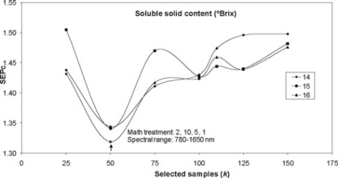
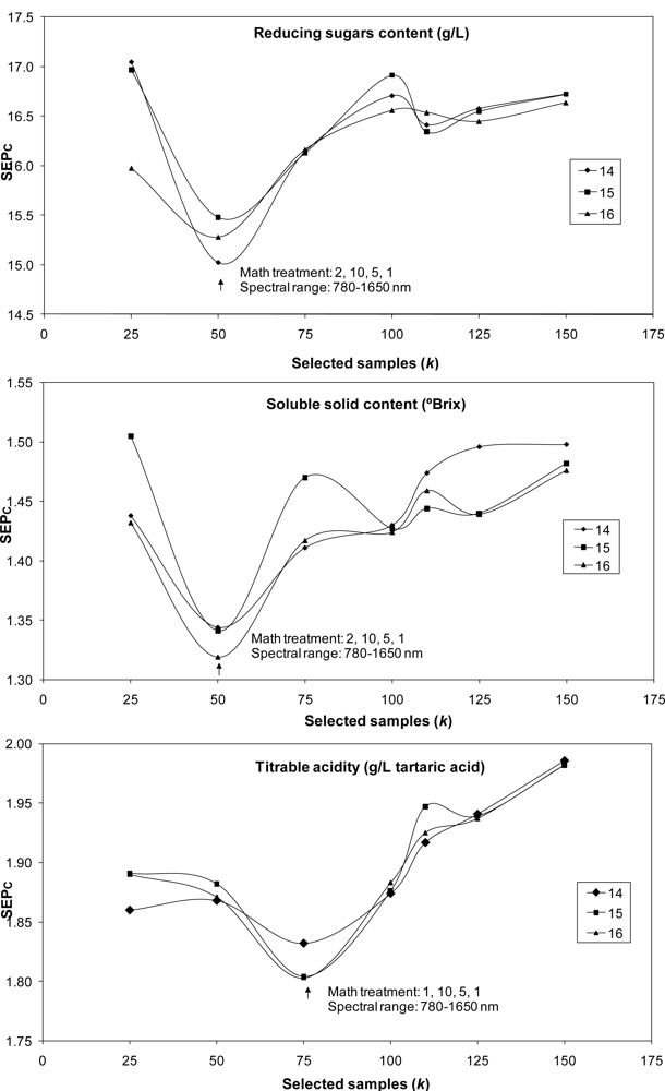
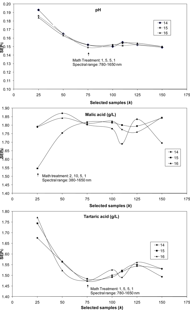
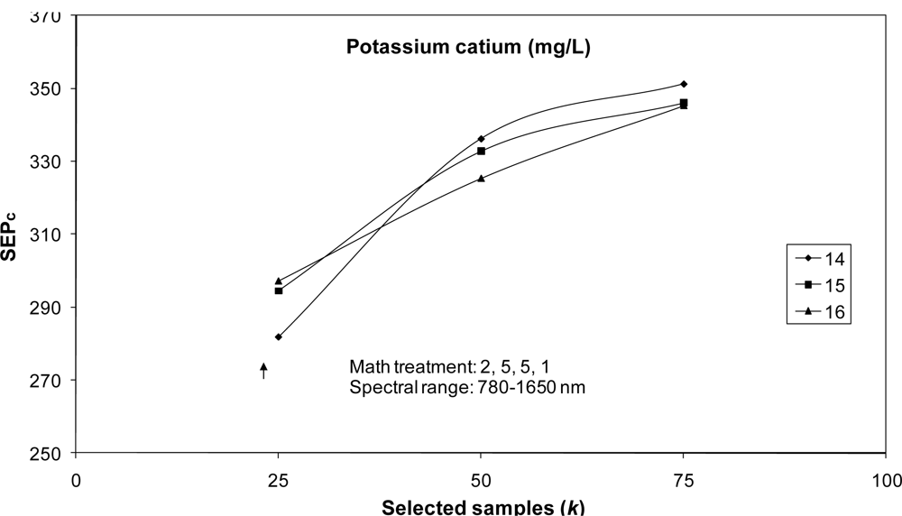
Different parameters have to be evaluated in order to optimize the LOCAL algorithm [24,25]. In the present study, for each dataset, an optimization design was set up by varying the number of calibration samples (k) from 25 to 150 in steps of 25, but including 110, for predicting SSC, reducing sugar content, pH-value, titratable acidity, tartaric acid, malic acid; and from 25 to 75 in steps of 25 for predicting potassium content in bunches; the number of PLS terms (l) was varied from 14 to 16 in steps of 1, where the number of predicted values corresponding to the first PLS terms discarded was 4. Finally, the minimum number of samples used for each calibration was set to 15.

For both algorithms, the following spectral regions were tested for calibration purposes: 380–1,650 nm (the highest spectral range with useful information covering the VIS + NIR regions); 780–1,650 nm (the highest spectral range covering the NIR region and including the very near infrared region) and 1,100–1,650 nm (including only the strict near-infrared region). In order to eliminate noise at the end of the spectral range, the region between 1,650–1,700 nm was discarded.

Mahalanobis distance statistics, H_global and H_neighbour, were computed from the principal components of the selected samples to check the accuracy of predictions [17,26]. The effect of the different settings on the performance of MPLS and LOCAL was evaluated by comparing the standard error of prediction (SEP), the coefficient of regression for the external validation (r²), the bias, and the standard error of prediction corrected for bias or SEP(c).

During ripening, the study parameters covered a relatively wide range, due to the constant changing of sample matrices. Changes in chemical composition are shown in Table 1, which also indicates the number of samples in the calibration and validation sets following application of the CENTER algorithm, together with mean, standard deviation (SD), and coefficient of variation (CV) values. Samples were collected over the critical months to check for variations in SSC (10.60–58.60 °Brix), titratable acidity (0.20–20.50 g/L tartaric acid) and tartaric acid (4.90–18.60 g/L tartaric acid) in the berry.

The sample set was highly variable, since it contained data from grapes sampled at different stages of ripening over three years; this accounts to a large extent for the high CV values recorded, particularly for SSC, reducing sugar content, titratable acidity, tartaric acid, malic acid and potassium content (Table 1). The results confirm the suitability of this method for selecting the validation set, since calibration and validation set displayed similar values for mean, SD, range and CV for all parameters studied, and the ranges for the validation set lay within the range recorded for the calibration set.

During veraison and until ripening, there is a progressive decline in malic, and to a lesser extent in tartaric acid levels. Flanzy [3] notes that tartaric acid is mostly formed in growing organs and cannot be metabolized except at temperatures over 35 °C. Since temperatures are highest at the end of ripening, it is at this stage when the lowest tartaric acid levels are recorded. Malic acid is synthesized following the combustion of sugars in chlorophyll-containing tissues. Unlike tartaric acid, it is unstable, and is metabolized during ripening, leading to low levels at harvest.

Potassium is the major mineral cation in grapes and plays a major role in the neutralization of tartaric and malic acid in the berries, thereby affecting the grape’s acid profile [27,28]. Potassium directly determines the pH not only of wine but also of must [29]. It is present in wines mainly as potassium bitartrate, an unstable compound that can precipitate at cool temperatures as a crystalline deposit [30].

The LOCAL algorithm was also used to predict internal quality parameters in bunches. The best SEPc values obtained with the best mathematical treatments and spectral ranges over 21 runs (7 values for k and 3 for l) are shown in Figure 1. The lowest values for SEPc were achieved with the lowest values for k. For application of the LOCAL strategy, only 25 samples were used to predict malic acid and potassium content; 50 samples were used for SSC and reducing sugar content predictions, and 75 samples were used for pH, titratable acidity and tartaric acid. Samples were selected as being the most representative of the calibration set, rather than using all the 251 samples or the 104 samples in the case of potassium cation employed to construct the calibration model using MPLS regression.

In most cases, the values selected for parameter l (number of PLS terms) had little influence on SEPc values; marked differences being observed only for SSC and malic acid. The best results achieved with the LOCAL algorithm were then compared with those obtained using MPLS regression for the prediction of the 93-sample validation set except for the potassium cation (n = 44), using only bunch analysis (Table 3).

It needs to point out that the sistematic procedure follows in this work is more favourable for the LOCAL algorithm, since the tuning of LOCAL was done on the validation set, with 21 combinations of parameters, being selected the one with best SEP, while the best MPLS model was chosen taking into account the cross validation statistics and only the best model applied to the validation set. Nevertheless, this systematic has been selected since the differences between the statistics obtained for the MPLS models were no-relevant, and also taking into account that cross-validation statistics, according to Shenk [23], give a realistic estimate of the error prediction of samples not included in the calibration.

The results obtained using LOCAL were better than those achieved using MPLS regression, in terms of both r² and SEPc, for total soluble solid content, reducing sugar content, pH, tartaric acid and potassium content, although the improvement was only slight for reducing sugar and tartaric acid content. For titratable acid and malic acid, application of the LOCAL algorithm improved model precision but also prompted a slight increase in SEPc values.

The improvement in r² values achieved using the non-linear strategy ranged between 2% for both tartaric acid and reducing sugar content and 41% for malic acid, while the improvement in SEPc values ranged from 1.5% for tartaric acid to 22% for SSC. Shenk [35] suggest that application of the LOCAL algorithm can improve the predictive capacity of models by 10–30%.

With regard to spectral range suitability, the best results using the LOCAL strategy were generally obtained in the 780–1,650 nm range, except for malic acid content; by contrast, MPLS yielded the best results for all parameters using a wider spectral range (380–1,650 nm), except for reducing sugar content. The optimal number of PLS terms for the prediction of each parameter using the LOCAL algorithm (Table 3) was always equal to or smaller than the optimal number using MPLS.