Fault Diagnosis for Micro-Gas Turbine Engine Sensors via Wavelet Entropy


Abstract
: Sensor fault diagnosis is necessary to ensure the normal operation of a gas turbine system. However, the existing methods require too many resources and this need can’t be satisfied in some occasions. Since the sensor readings are directly affected by sensor state, sensor fault diagnosis can be performed by extracting features of the measured signals. This paper proposes a novel fault diagnosis method for sensors based on wavelet entropy. Based on the wavelet theory, wavelet decomposition is utilized to decompose the signal in different scales. Then the instantaneous wavelet energy entropy (IWEE) and instantaneous wavelet singular entropy (IWSE) are defined based on the previous wavelet entropy theory. Subsequently, a fault diagnosis method for gas turbine sensors is proposed based on the results of a numerically simulated example. Then, experiments on this method are carried out on a real micro gas turbine engine. In the experiment, four types of faults with different magnitudes are presented. The experimental results show that the proposed method for sensor fault diagnosis is efficient.1. Introduction
Gas turbines are one of the most important types of power equipment, widely used in modern aircraft propulsion systems and power systems. In order to achieve their challenging customer-driven performance requirements, gas turbines have to operate at their physical limits, which are set by material and gas properties. However, the normal operations of the gas turbines rely on the fine tuned cooperation of many different components, and any minor problem with these components may adversely affect the gas turbine system. Thus, advanced controls and monitoring technologies to improve the safety and reliability of the gas turbine system are widely studied, and at the same time, to reduce the operating cost.
The control and monitoring of gas turbine systems depend on accurate and reliable sensor readings from a considerable number of sensors. All these sensors must be functional to ensure normal operation of a gas turbine, otherwise, sensor failures may mislead the controller, and lead to the paralysis of the entire system. Therefore, in order to improve the reliable operation of systems, it is necessary to employ sensors fault diagnosis in a timely and accurate fashion.
For the reasons described above, sensor fault diagnosis has received considerable attention and many works on this topic have been reported. Isermann [1] presented an extended review of the field of fault detection and diagnosis, in which many fault detection and diagnosis methods were presented. Botros et al. [2] proposed an application of radial basis function neural networks for sensor fault detection on an RB211 gas turbine driven compressor station. Napolitano et al. [3] discussed the performance of a simulated neural network based fault-tolerant flight control system for sensor fault detection. Dewallef and Leonard [4] worked out a methodology for on-line sensor validation in turbojet engines using neural networks for generation of the mathematical representation of the engine. Ogaji et al. [5] reported a multiple sensor fault diagnoses method for a 2-shaft stationary gas turbine. Romesis et al. [6] presented a sensor fault detection method based on a probabilistic neural network. Aretakis et al. [7] reported an approach for detecting sensor faults in turbofan engines. Mehranbod et al. [8] presented a Bayesian belief network (BBN)-based sensor fault detection and identification method. Palmé et al. [9] also presented recently a similar solution for sensor validation based on artificial neural networks.
With increasing demand on small power systems and small propulsion systems, many micro gas turbines are being developed, and excellent success has been achieved in this area. However, the power to weight ratio of a micro-gas turbine should be high, so its EEC (electronic engine controller) should be light and have low power consumption, thus the microcontroller in the EEC is not powerful enough to adopt nonlinear engine model or neural networks for sensor validation. Consequently, the previous approaches are not suitable for micro-gas turbines. To overcome such problems, a simple and efficient approach should be adopted.
Typically, there are five types of sensor faults: the step fault (including the open and short fault), the pulse fault, the periodic fault, the noise fault and the drift fault. If any type of fault occurs, except for the drift fault, transient readings from the sensor will be affected. Thus, the fault status of the sensor could be extracted by analyzing the sensor readings. A mature and efficient tool for signal analysis is Fourier analysis, which transforms the sensor signal from a time-based domain to a frequency-based one. However, it is hard to determine when a particular fault takes place. To improve this deficiency, Gabor proposed the short-time Fourier transform (STFT) [10]. The windowing technique analyzes a small section of signal each time. The STFT maps a signal into a 2-D function of time and frequency. Still, the transformation has disadvantage that the time or frequency information can only be obtained with limited precision, which is determined by the size of the window. A higher resolution in both time and frequency domain cannot be achieved simultaneously since once the window size is fixed, which is the same for all frequencies. The wavelet transform (WT) is a popular technique to analyze signals. Wavelet functions are composed of a family of basis functions that are capable of describing a signal in both the time and frequency domains [11]. To enhance the performance of the wavelet transform, the concept of wavelet entropy is introduced in feature extraction. The method is widely used in many fields, and has achieved considerable success [12–16].
This paper proposes a fault diagnosis method for micro-gas turbine sensors operating under nonstationary conditions. The fault types mentioned above are investigated, except for drift faults. Based on wavelet theory, wavelet decomposition is utilized to decompose the signal in different scales. Then the instantaneous wavelet energy entropy (IWEE) and instantaneous wavelet singular entropy (IWSE) are defined based on the previous wavelet entropy theory. Subsequently, a fault diagnosis method for gas turbine sensors is proposed based on the numerically simulated example. Finally, experiments are carried out on this method, and the results show that it is efficient.
2. Theoretical Background
2.1. Wavelet Transform [11]
Wavelets are finite-energy functions with good localization properties in both the frequency and time domain, which can be used very efficiently to represent transient signals. For a given mother wavelet ψ(t), a scaled and translated version (wavelet family) is designated by:
For a given signal f(t) ∈ L2(ℝ), the results of the wavelet transform are the correlation between the function f(t) with the family wavelet ψa,b for each a and b:
By selecting a special mother wavelet function ψ(t) and the discrete set of parameters (aj = 2−j, bj,k = 2−jk, j,k ∈ Z), the wavelet family could be presented as:
The discrete wavelet transform (DWT) of signal f(t) can be obtained through Equation (4).
2.2. Wavelet Decomposition and Wavelet Entropy
In 1989 Mallat presented a fast wavelet decomposition algorithm for discrete wavelet transform, which utilizes the orthogonal wavelet bases to decompose the signal under different scales [17]. It is equivalent to recursively filtering a signal with a high-pass and low-pass filter pair which gives the detailed components and approximation components, respectively.
By using Mallat’s mathod, a certain time serise x(k) (k = 1, 2,…, N) could be decomposed as:
The frequency band of Aj(k) and Dj(k) could be represented by:
Since the wavelet bases used to decompose the signal are orthogonal, these decomposed signals could be regarded as a direct estimation of local energies at different scales [17]. Thus, the wavelet engery of detailed components at instant k and scale j will be represented as:
For the purpose of unification, the wavelet engery of approximation components at instant k and scale J is defined as:
Consequently, the wavelet engery at each sacle (J + 1 scale means approximation components) could be described as:
The total wavelet engery could be defined as:
2.3. Wavelet Entropy
The concept of entropy is derived from thermodynamic entropy, which can be roughly seen as a measure of the degree of system chaos. In the information world, Shannon defined the Shannon entropy that can represent the degree of chaos of a system [18]. It provides an efficient criterion for analyzing and comparing probability distributions. Given a random variable X which takes a finite number of possible values x1, x2, …, xn with probabilities p1, p2, …, pn respectively, where pi ≥ 0, i = 1,2, …, n and . The Shannon entropy could be written as:
The concept of wavelet entropy is inherited from Shannon entropy. Many types of wavelet entropies have been defined to solve different problems, and these methods can achieve good detection and recognition performance. Blanco et al. [12] defined wavelet entropy based on wavelet transform in 1998 and applied it to analyse electroencephalography traces. He et al. [13] defined several kinds of wavelet entropy to analyse transient signals in power systems. Ren et al. [16] proposed a method for structural damage identification via wavelet entropy.
The wavelet entropy proposed above can represent the degree of order/disorder of the measured signal from sensors, which can provide useful information about the underlying state of the sensors. However, in critical circumstanced, such as gas turbine operation, sensor faults should be detected immediately. Gathering a large number of sensor readings and performing a post-analysis is not practical. Thus, it is necessary to define a type of instantaneous wavelet entropy to solve this problem. Based on the definition in [13], the instantaneous wavelet energy entropy (IWEE) and instantaneous wavelet singular entropy (IWSE) are defined as follows.
To obtain the instantaneous wavelet entropy of x(n) at instant k, a window of the time series is picked out, i.e., xw(n) = x(k − W + 1),…, x(k), k − W + 1 > 0, where W is the width of the window. More information could be obtained when a higher vaule of W is chosen, however, this implies more calculation costs, thus, the proper value of W should be considered. Decomposing xW(n) via wavelet decomposition, then a series of signal at different scale could be produced as:
As defined in Equation (5) the wavelet energy of xW(n) at each scale and total could be represented as in Equations (13) and (14):
Thus, we define the normalized pj, with pj = EWj/EWtol, j = 1,2, …, J + 1 and ∑jpj = 1, which represents the distribution of wavelet energy at different scales. According to Equation (11), the IWEE at instant k will be defined as:
As mentioned above, the approximation components and detailed components could be obtained through wavelet decompositions, and the detailed componets contain high frequency information of the original siganl. As we all know, a mutation will occur in the measured sensor signal when the sensor fails, and this mutational signal lies in the detailed components certainly. Thus, the IWSE is defined based on the detailed components, which aims to uncover the fault information contained in the sensor signal.
As described in Equation (12), detailed components of the decomposed signal can constitute a W × J matrix D, where W is the width of the slide window and J means scale number. According to the singular value decomposition theory, there exist a W × l matrix U, an l × J matrix V and an l × l matrix Λ, which could make the relationship given in Equation (16):
The diagonal elements λi(i = 1,2,…,l) of the diagonal matrix Λ are not negative and in descending order. These diagonal elements are the singular values of the matrix D. As described in the signal singular value decomposition theory, when the signal has no noise or high signal-to-noise ratio, only a few diagonal elements exist. Thus, these diagonal elements could be employed to extract information about the frequency distribution at different scales, so a variable qj is defined as Equation (17), where qj > 0, ∑lqj = 1, j = 1, 2, …, l, and the IWSE at instant k is defined as Equation (18):
3. Sensor Fault Diagnosis Method Based on Wavelet Entropy
3.1. Numerically Simulated Example
To illustrate the fault diagnosis ability by the proposed IWWE and IWSE, the following numerical simulations are investigated. Given a stationary signal S(t) = (2 + N(0,0.04))V (0 ≤ t < 10s), where N(0,0.04) is Gaussian white noise with covariance 0.04, which stands for the stationary signal from a normal sensor. To represent the signal with faults, several kinds of fault signals, such as pulse fault, noise fault, periodic fault and step fault signals, are added in to S(t), then the new siganl f(t) could be represented as:
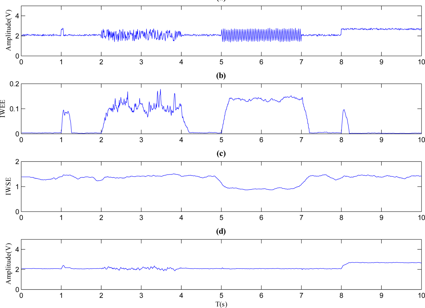
Sampling f(t) with a frequency of 100 Hz, a discrete verison of signal f(n) can be produced. Let the mother wavelet type be ‘haar’ wavlet (requiring less calculation), W = 20 and J = 5, then the time series f(n) is decomposed, at the same time, the IWEE and IWSE are calculated. The corresponding results are shown in Figure 1. Figure 1(a) represents the discrete time series f(n), while Figure 1(b,c) stand for the IWEE curve and IWSE curve separately. Figure 1(d) presents the curve of mean value of approximation components at J scale. According to Equation (12), the mean value of approximation components at J scale at instant k can be represented as:
As shown in Figure 1(b), the IWEE value mutates and grows where the fault signals are mixed in, which can indicates when the faults occur. Meanwhile, the IWEE value changes and returns to normal quickly when a pulse or step fault occurs. However, the IWEE value changes and stays for a while when a noise or periodic fault occurs. Since the IWEE value pattern when a pulse or step fault occurs is identical, the Amean(n) could be employed to distinguish them as shown in Figure 1(d). The Amean(n) will be changed when a step fault occurs. Similarly, noise or periodic faults could be distinguished through IWSE. As Figure 1(c) shows, the IWSE value goes low when a periodic fault happens, however it is steady when a noise fault occurs. As the result of numerically simulated example shown, the proposed IWEE and IWSE are good tools for fault diagnosis.
3.2. Proposed Method for Sensor Fault Diagnosis Based on Wavelet Entropy
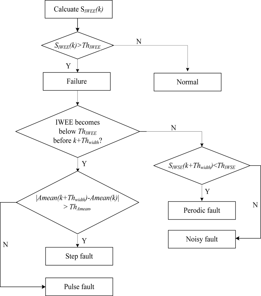
The sensor fault diagnosis method is proposed based on the results of the numerical simulations. In order to explain the method clearly, several parameters are defined in Table 1. The proposed sensor fault diagnosis method is shown in Figure 2.
Step 1. Combine the sensor reading at time k with the W−1 samples gathered previously, then a new time series with the length W could be obtained, which is presented as x(n), (n = k − W + 1, …, k).
Step 2. Figure out the IWEE of x(n) and compare it with the ThIWEE, the sensor is judged to be faulty when IWEE is more than ThIWEE, otherwise the sensor is normal.
Step 3. Monitor the value of IWEE, if it becomes less than ThIWEE before time k + Thwidth is reached, the fault is a pulse or step type fault (CASE 1), otherwise, the fault type should be a noise or periodic fault (CASE 2). At the same time, calcuate the Amean and IWSE from time k to k + Thwidth.
Step 4. For CASE 1 in Step 3, check if SIWSE (k + Thwidth) < ThAmean, if yes the fault type is noise, otherwise the fault type is periodic. For CASE 2 in Step 3, check if | Amean(k + Nd) − Amean(k)| > ThAmean, if yes the fault type is step, otherwise the fault type is pulse.
4. Experiments on a Micro Gas Turbine Engine
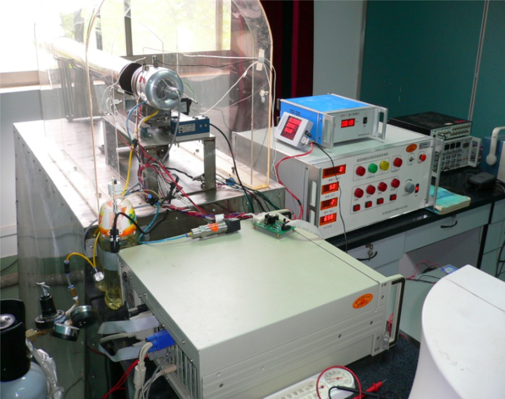
The experiments for the proposed method are carried out on the “Chao Ying” engine, which is a single shaft micro-gas turbine developed at the Nanjing University of Aeronautics and Astronautics. The temperature sensor placed in the nozzle is employed to verify the proposed sensor fault diagnosis method. In our system, the temperature sensor is made from a platinum thermocouple, and the temperature range that can be sensed by it is from 0 to 1,600 °C, and the output of the sensor is adjusted to 0 to 5 V. The environment for experiments is shown in Figure 3. To carry out the experiments, the output of the temperature sensor is sampled and then forwarded to a PC through a RS232 serial port. To simulate the output of a sensor with fault, various types of faults were artificially added using software.
In this experiment, the main parameters for the method are chosen as listed in Table 2. In order to demonstrate the performance of the proposed method in a practical situation, the micro-gas turbine engine is set to work under nonstationary conditions by adjusting the angle of the throttle lever. Thus, the the measured signal of the sensor is dynamic and similar to what would be encountered under practical conditions. To form fault signals artificially, four types of faults (pulse, step, noise and periodic) are added into the normal time series separately.
Considering minimum detectable fault magnitude (MDFM) is an important parameter for the proposed method, and it is also a significant index of practicality. Henceforth, the minimum detectable fault magnitude for the proposed method should be determined through the experiment, so in the following experiment, four types of faults with 1%, 5%, 10% and 15% magnitude variations are presented. The detailed analysis is as follows.
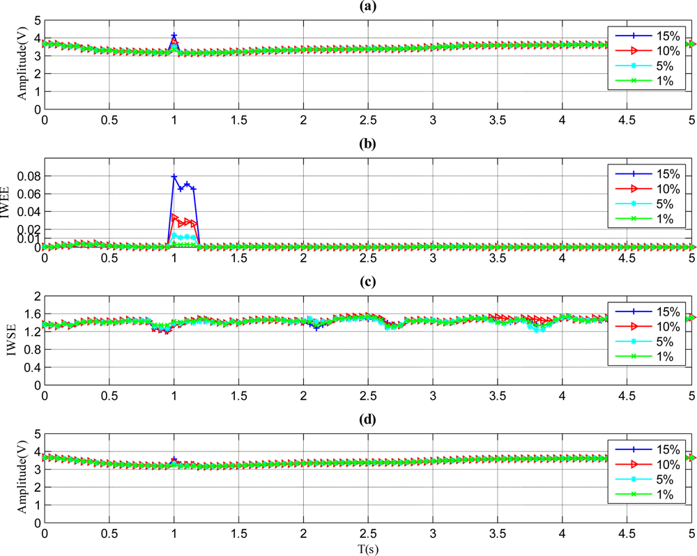
The results of a sensor with a pulse fault are described in Figure 4. As shown in Figure 4(b), the IWEE value grows higher than ThIWEE when the fault magnitude is 5%, 10% or 15%. However, the IWEE value is below ThIWEE when the fault magnitude is 1%, thus the fault with 1% fault magnitude is undetectable through the proposed method. Therefore, the MDFM for this kind of fault is regarded as 5%. Furthermore, the Amean value in Figure 4(d) barely varies when the faults occur, so the fault type is determined to be pulse, which is identical to Figure 2.
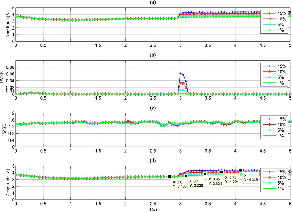
The results of a sensor with step fault are illustrated in Figure 5. Like Figure 4(b), the IWEE value of each magnitude variation grows when the faults occur in Figure 5(b). In Figure 5(d), the increased Amean value is more than ThAmean when the fault signal amplitude is 5%, 10% or 15%, so the fault type is identified to be step according to Figure 2. However, the increased Amean value is lower than ThAmean when the fault signal amplitude is 1%, so the MDFM for the step fault is also set at 5%.
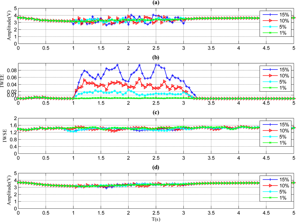
The results of sensor with noise fault are illustrated in Figure 6. As shown in Figure 6(b), the IWEE value of each magnitude variation grows and remains until the fault disappears. For this duration, the IWEE value stays higher than ThIWEE when the fault magnitude is 5%, 10% or 15%, but is less than ThIWEE when the fault magnitude is 1%, so the fault with 1% fault magnitude is undetectable by the proposed method, and the proper MDFM for the this fault type should be 5%. As to the IWSE shown in Figure 6(c), the IWSE values for all magnitude variations stay higher than ThIWSE, thus the fault type is identified to be noise, according to Figure 2.
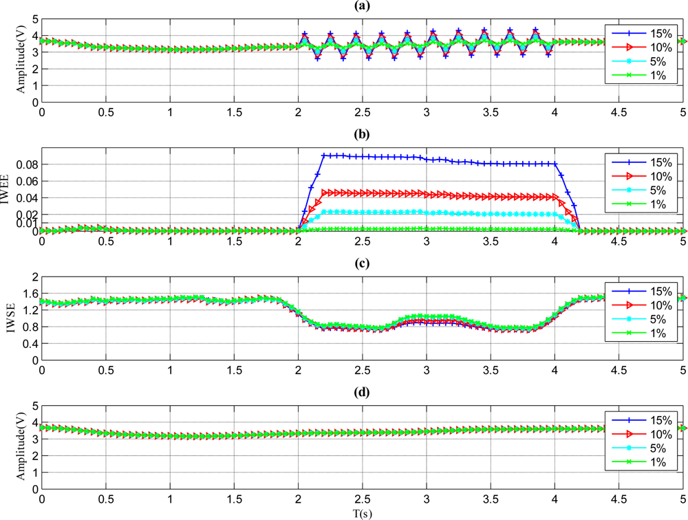
Figure 7 represents the situation for a periodic fault. As shown in Figure 7(b), the IWEE value of each magnitude variation goes higher than ThIWEE and stays there until the faults recover when the fault magnitude is 5%, 10% or 15%, while it remains lower than ThIWEE when the fault magnitude is 1%. Therefore, the fault with 1% fault magnitude is undetectable by the method, and the proper MDFM for this fault type is 5%. As shown in Figure 7(c), the IWSE values of all situations become lower than the fault duration, so the fault type is identified to be periodic according to Figure 2.
4. Conclusions
The status of a sensor can be reflected by its output signal, hence it is feasible to perform sensor fault diagnosis by analysing the measured sensor signals. This paper proposes a method for sensor fault diagnosis via wavelet entropy. Based on the wavelet theory, two types of wavelet entropies, IWEE and IWSE, are defined to extract the inherent sensor information. Then a method using of IWEE and IWSE as criteria is presented. In order to verify the performance of the proposed method, an experiment is carried out on an actual micro-gas turbine engine. In the experiment, four types of faults with different magnitudes are presented. The results show that the proposed method is efficient for senor fault diagnosis.
The proposed sensor fault diagnosis method has some limitations that require improvement. Firstly, the types of sensor faults verified are limited, and more types of sensor faults should be tested via the method. Meanwhile, the values in Table 2 are chosen for particular sensor, which should be verified by more practical data. Finally, the proposed method is guaranteed to work only when the amplitude of fault signal is more than 5% of full scale, so some improvements must be done to enhance its performance.
Acknowledgments
This work has been partially supported by the Startup Foundation of Nanjing University of Aeronautics and Astronautics (No. S0956-021).
References
- Isermann, R. Supervision, fault-detection and fault-diagnosis methods—An introduction. Control Eng. Pract 1997, 5, 639–652. [Google Scholar]
- Botros, KK; Kibrya, G; Glover, A. A demonstration of artificial neural-networks-based data mining for gas-turbine-driven compressor stations. J. Eng. Gas Turb. Power 2002, 124, 284–297. [Google Scholar]
- Napolitano, MR; An, Y; Seanor, BA. A fault tolerant flight control system for sensor and actuator failures using neural networks. Aircr. Des 2000, 3, 103–128. [Google Scholar]
- Dewallef, P; Leonard, O. On-line validation of measurements on jet engines using automatic learning methods. Proceedings of the 15th ISABE Conference, Bangalore, India, 13–15 December 2001; pp. 1–8.
- Ogaji, SOT; Singh, R; Probert, SD. Multiple-sensor fault-diagnoses for a 2-shaft stationary gas-turbine. Appl. Energ 2002, 71, 321–339. [Google Scholar]
- Romesis, C; Mathioudakis, K. Setting up of a probabilistic neural network for sensor fault detection including operation with component faults. J. Eng. Gas Turb. Power 2003, 125, 634–641. [Google Scholar]
- Aretakis, N; Mathioudakis, K; Stamatis, A. Identification of sensor faults on turbofan engines using pattern recognition techniques. Control Eng. Pract 2004, 12, 827–836. [Google Scholar]
- Mehranbod, N; Soroush, M; Panjapornpon, C. A method of sensor fault detection and identification. J. Process Control 2005, 15, 321–339. [Google Scholar]
- Palmé, T; Fast, M; Thern, M. Gas turbine sensor validation through classification with artificial neural networks. Appl. Energ 2011, 88, 3898–3904. [Google Scholar]
- Gabor, D. Theory of communication. J. Inst. Elect. Eng 1946, 93, 429–457. [Google Scholar]
- Daubechies, I. Ten Lectures on Wavelets; Society for Industrial and Applied Mathematics: Philadelphia, PA, USA, 1992. [Google Scholar]
- Blanco, S; Figliola, A; Quiroga, RQ; Rosso, OA; Serrano, E. Time-frequency analysis of electroencephalogram series. III. Wavelet packets and information cost function. Phys. Rev. E 1998, 57, 932–940. [Google Scholar]
- He, ZY; Chen, XQ; Luo, GM. Wavelet entropy measure definition and its application for transmission line fault detection and identification. Proceedings of 2006 International Conference on Power Systems Technology, Chongqing, China, 22–26 October 2006; pp. 634–639.
- He, ZY; Gao, SB; Chen, XQ; Zhang, J; Bo, ZQ; Qian, QQ. Study of a new method for power system transients classification based on wavelet entropy and neural network. Int. J. Elect. Power 2011, 33, 402–410. [Google Scholar]
- Rosso, OA; Martin, MT; Figliola, A; Keller, K; Plastino, A. Eeg analysis using wavelet-based information tools. J. Neurosci. Meth 2006, 153, 163–182. [Google Scholar]
- Ren, W-X; Sun, Z-S. Structural damage identification by using wavelet entropy. Eng. Struct 2008, 30, 2840–2849. [Google Scholar]
- Mallat, SG. A theory for multiresolution signal decomposition: The wavelet representation. IEEE Trans. Patt. Anal. Mach. Intell 1989, 11, 674–693. [Google Scholar]
- Shannon, CE. A mathematical theory of communication. Bell Syst. Tech. J 1948, 27, 379–423. [Google Scholar]


| Parameters | Discription |
|---|---|
| ThIWEE | The threshold of IWEE value to ckeck if any fault exists. |
| Thwidth | The threshold to distinguish if the mutation of IWEE value keeps higher than ThIWEE for a certain time or not. |
| ThIWSE | The threshold of IWSE value to distinguish whether the fault type is noise or perodic. |
| ThAmean | The threshold of changed value of Amean to distinguish whether the fault type is step or pulse. |
| Parameters | Value |
|---|---|
| Sample frequency | 100 Hz |
| W | 20 |
| J | 5 |
| Mother wavelet | ‘Haar’ |
| ThIWEE | 0.01 |
| Thwidth | 60 |
| ThIWSE | 1.15 |
| ThAmean | 0.3 |
© 2011 by the authors; licensee MDPI, Basel, Switzerland. This article is an open access article distributed under the terms and conditions of the Creative Commons Attribution license (http://creativecommons.org/licenses/by/3.0/).
Share and Cite
Yu, B.; Liu, D.; Zhang, T. Fault Diagnosis for Micro-Gas Turbine Engine Sensors via Wavelet Entropy. Sensors 2011, 11, 9928-9941. https://doi.org/10.3390/s111009928
Yu B, Liu D, Zhang T. Fault Diagnosis for Micro-Gas Turbine Engine Sensors via Wavelet Entropy. Sensors. 2011; 11(10):9928-9941. https://doi.org/10.3390/s111009928
Chicago/Turabian StyleYu, Bing, Dongdong Liu, and Tianhong Zhang. 2011. "Fault Diagnosis for Micro-Gas Turbine Engine Sensors via Wavelet Entropy" Sensors 11, no. 10: 9928-9941. https://doi.org/10.3390/s111009928