Spectral Identification of Lighting Type and Character

Abstract
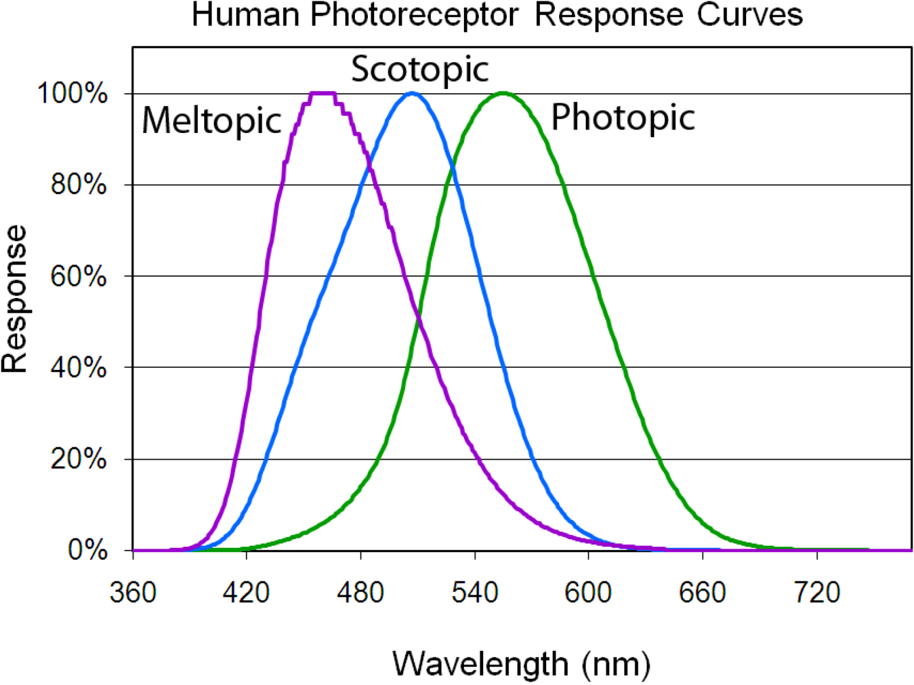
:
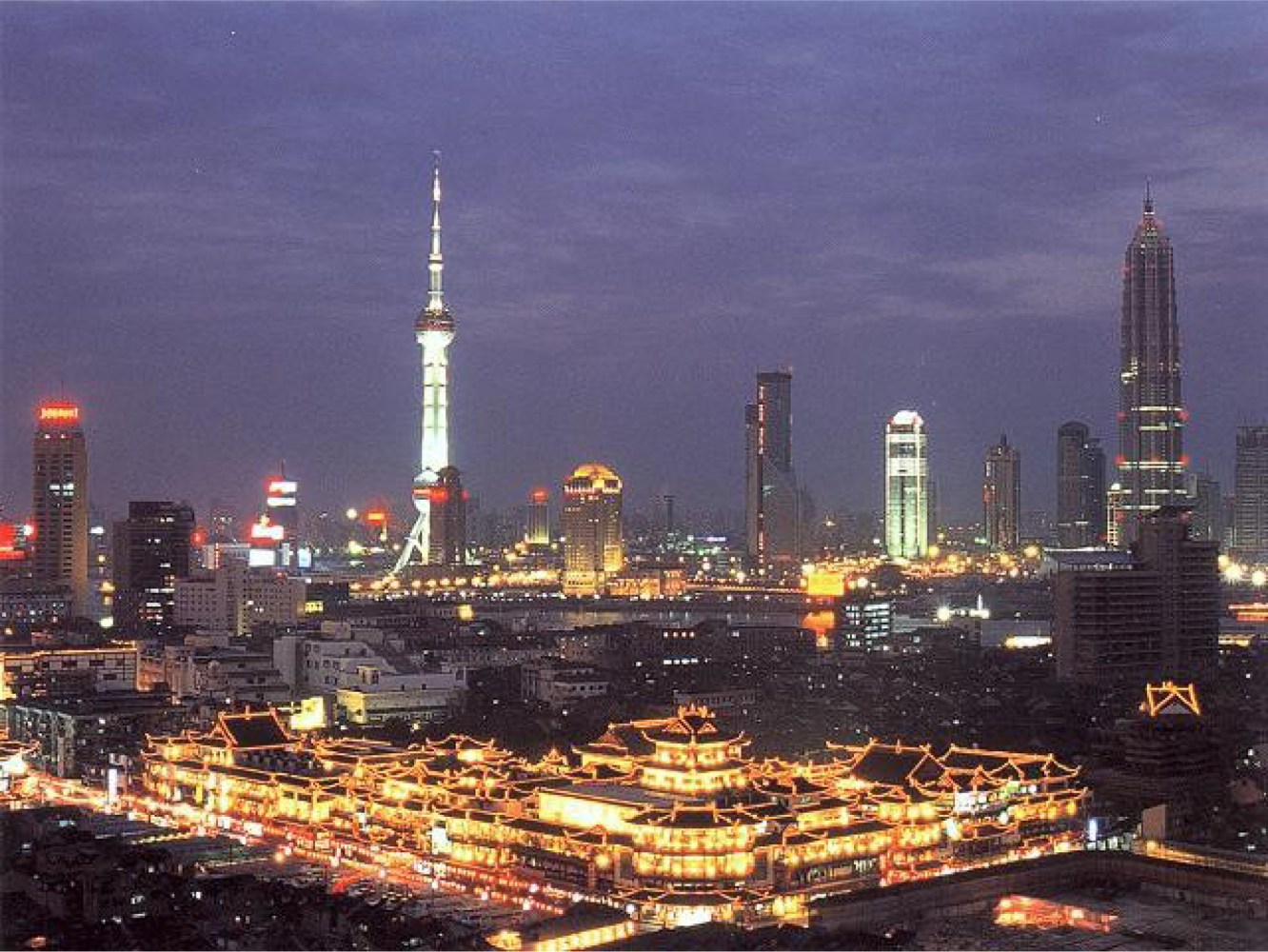
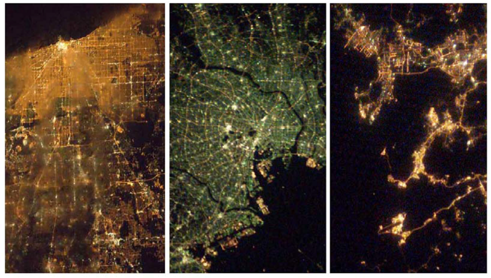
1. Introduction
“How many economists does it take to change a light bulb? None — market forces change light bulbs.”
2. Methods
2.1. Collection of Emission Spectra
2.2. Processing to Spectral Bands
3. Results
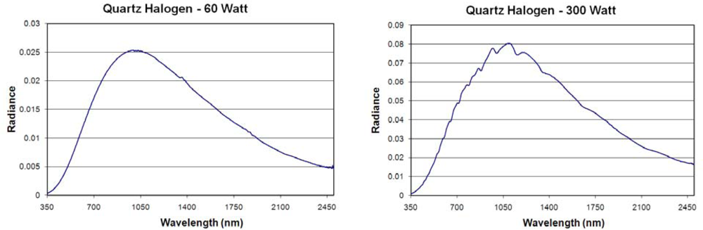
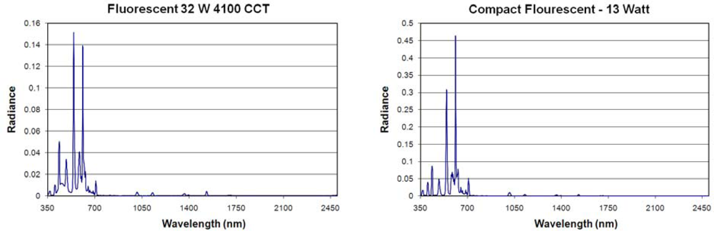
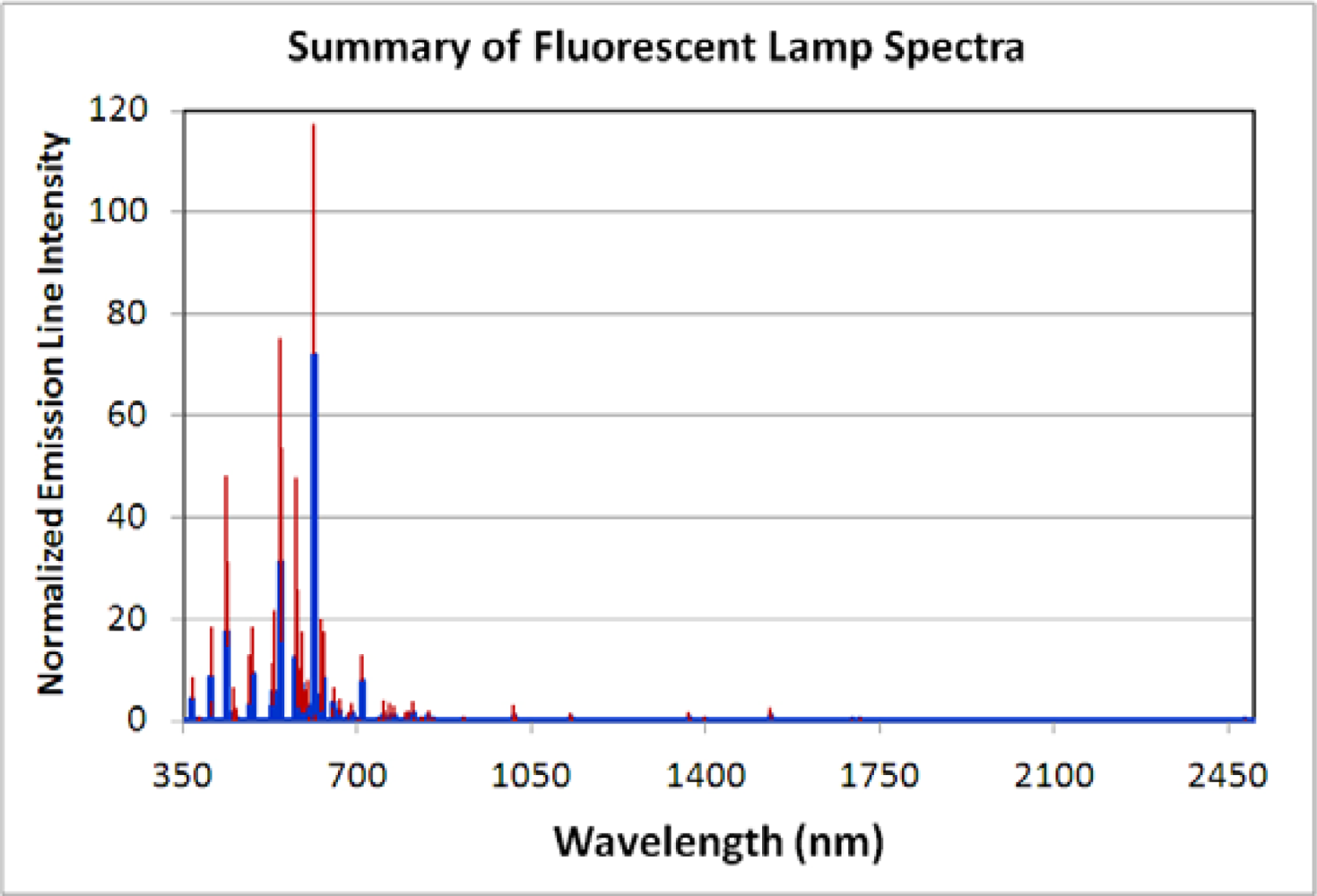
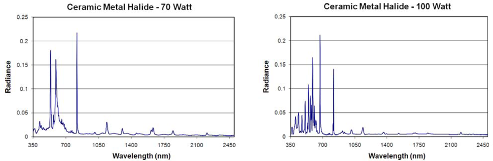
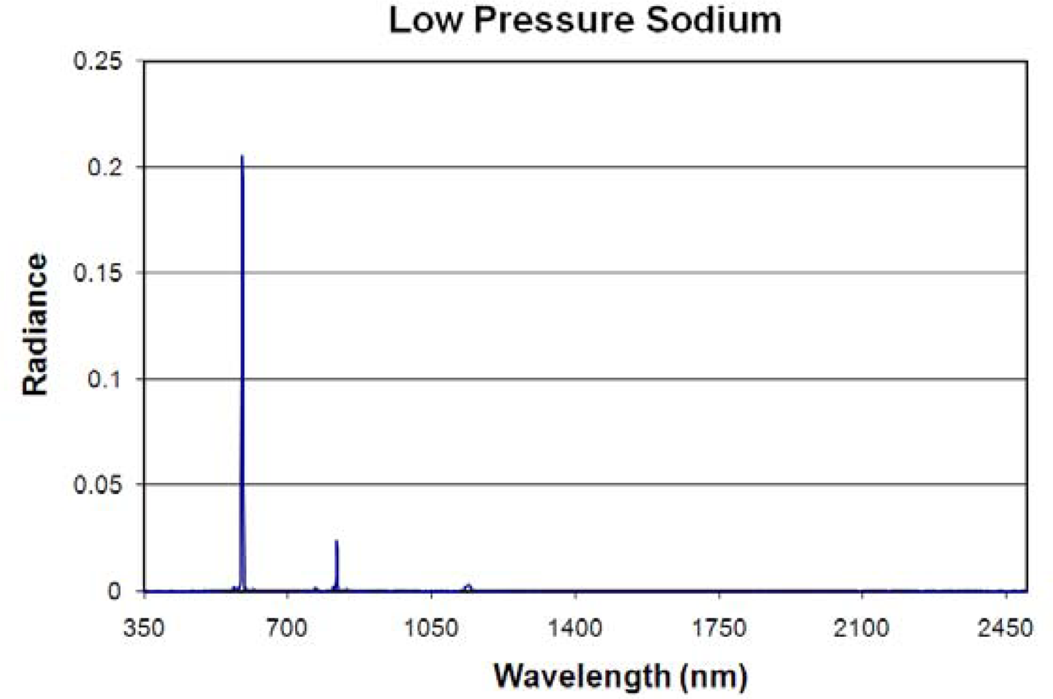
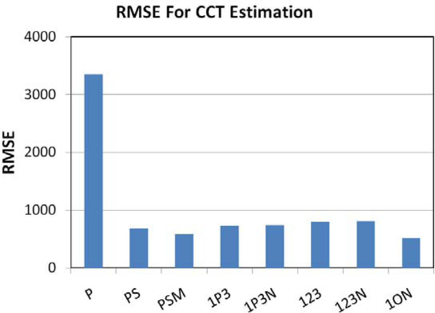
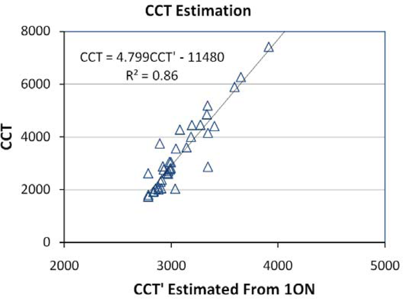
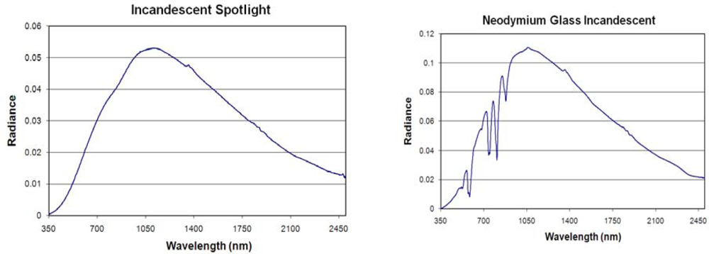
3.1. Spectral Characteristics of the Lamps
3.2. Discrimination of Lighting Types
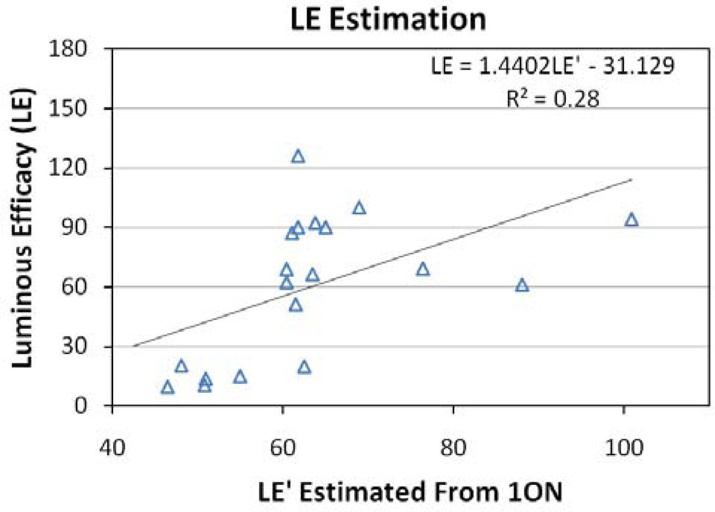
3.3. Estimation of Luminous Efficacy
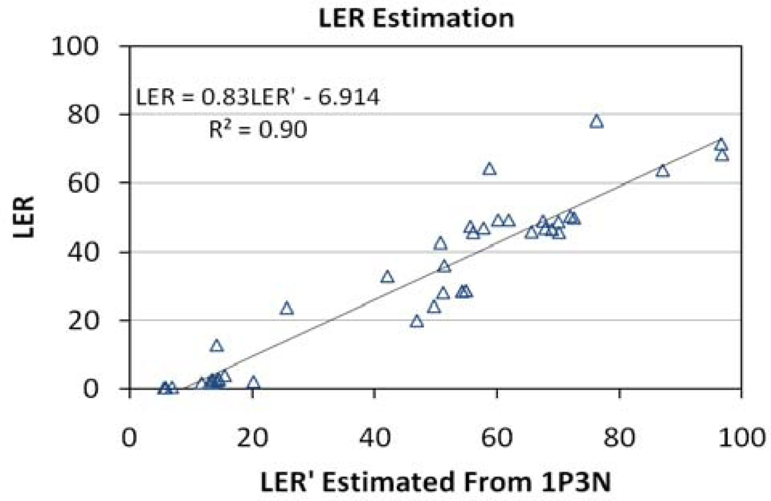
3.4. Luminous Efficacy of Radiation (LER):
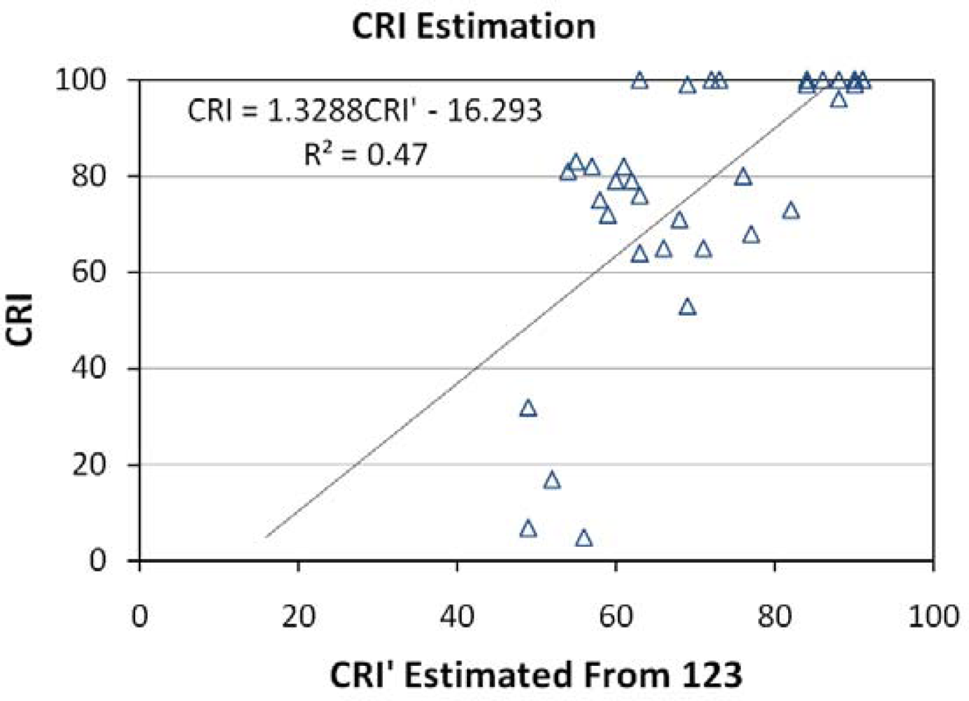
3.6. Color Rendering Index (CRI):
4. Conclusion
Acknowledgments
References and Notes
- International Energy Agency. Light’s Labour Lost; Paris, France, 2006. [Google Scholar]
- Mills, E. The specter of fuel based lighting. Science 2005, 308, 1263–1264. [Google Scholar]
- Rich, C.; Longcore, T. Ecological Consequences of Artificial Night Lighting; Island Press: Washington, DC, USA, 2005. [Google Scholar]
- Schubert, E.F.; Kim, J.K. Solid state light sources getting smarter. Science 2005, 308, 1274–1278. [Google Scholar]
- Croft, T.A. Night-time images of the earth from space. Sci. Amer 1978, 239, 68–79. [Google Scholar]
- Cinzano, P.; Falchi, F.; Elvidge, C.D. The first world atlas of the artificial night sky brightness. Mon. Notices Royal Astron. Soc 2001, 328, 689–707. [Google Scholar]
- Elvidge, C.D.; Tuttle, B.T.; Sutton, P.C.; Baugh, K.E.; Howard, A.T.; Milesi, C.; Bhaduri, B.; Nemani, R. Global distribution and density of constructed impervious surfaces. Sensors 2007, 7, 1962–1979. [Google Scholar]
- Center for International Earth Science Information Network (CIESIN), Columbia University; and Centro Internacional de Agricultura Tropical (CIAT). Gridded Population of the World Version 3 (GPWv3): Population Grids. Socioeconomic Data and Applications Center (SEDAC), Columbia University: Palisades, NY, 2005. Available online: http://sedac.ciesin.columbia.edu/gpw/ (accessed on 6 April 2010).
- Elvidge, C.D.; Sutton, P.C.; Ghosh, T.; Tuttle, B.T.; Baugh, K.E.; Bhaduri, B.; Bright, E. A global poverty map derived from satellite data. Comput. Geosci 2009, 35, 1652–1660. [Google Scholar]
- Elvidge, C.D.; Baugh, K.E.; Sutton, P.C.; Bhaduri, B.; Tuttle, B.T.; Ghosh, T.; Ziskin, D.; Erwin, E.H. Who’s in the Dark: Satellite Based Estimates of Electrification Rates. In Urban Remote Sensing: Monitoring, Synthesis and Modeling in the Urban Environment; Yang, X.J., Ed.; Wiley-Blackwell: Chichester, UK, In Press.
- Sutton, P.C.; Anderson, S.A.; Elvidge, C.D.; Tuttle, B.T.; Ghosh, T. Paving the planet: impervious surface as proxy measure of the human ecological footprint. Prog. Phys. Geog 2009, 33, 510–527. [Google Scholar]
- Elvidge, C.D.; Cinzano, P.; Pettit, D.R.; Arvesen, J.; Sutton, P.; Small, C.; Nemani, R.; Longcore, T.; Rich, C.; Safran, J.; Weeks, J.; Ebener, S. The Nightsat mission concept. Int. J. Remote Sens. 2007, 28, 2645–2670. [Google Scholar]
- Elvidge, C.D.; Safran, J.; Tuttle, B.; Sutton, P.; Cinzano, P.; Pettit, D.; Arvesen, J.; Small, C. Potential for global mapping of development via a Nightsat mission. GeoJournal 2007, 69, 45–53. [Google Scholar]
- CIE 1924. Commission Internationale de l’Éclairage Proceedings; Cambridge University Press: Cambridge, UK, 1926.
- CIE 1951. Commission Internationale de l’Éclairage Proceedings; Bureau Central de la CIE: Paris, France, 1951; pp. 37–39.
- Vogelmann, J.E.; Helder, D.; Morfitt, R.; Choate, M.J.; Merchant, J.W.; Bulley, H. Effects of Landsat 5 Thematic Mapper and Landsat 7 Enhanced Thematic Mapper Plus radiometric and geometric calibrations and corrections on landscape characterization. Remote Sens. Environ 2001, 78, 55–70. [Google Scholar]
- Pettit, D. Cities at night: an orbital perspective. NASA Ask Magazine 2010. In Press.. [Google Scholar]
- Lyon, R.J.P. Analysis of rocks by spectral infrared emission (8 to 25 microns). Economic Geology 1965, 60, 715–736. [Google Scholar]
- Wilson, W.H.; Kiefer, D.A. Reflectance spectrosopy of marine-phytoplankton 2. Simple-model of ocean color. Limnol. Oceanogr 1979, 24, 673–682. [Google Scholar]
- Milton, N.M. Use of reflectance spectra of native plant-species for interpreting airborne multispectral scanner data in the East Tintic Mountains, Utah. Economic Geology 1983, 78, 761–769. [Google Scholar]
- Elvidge, C.D. Visible and near-infrared reflectance characteristics of dry plant materials. Int. J. Remo. Sens 1990, 11, 1775–1795. [Google Scholar]
- Provencio, I.; Jiang, G.; De Grip, W.J.; Hayes, W.P.; Rollag, M.D. Melanopsin: An opsin in melanophores, brain, and eye. Proc. Nat. Acad. Sci 1998, 95, 340–345. [Google Scholar]
- He, S.; Dong, W.; Deng, Q.; Weng, S.; Sun, W. Seeing more clearly: Recent advances in understanding retinal circuitry. Science 2003, 302, 408–411. [Google Scholar]
- Hollan, J. Metabolism-influencing light: measurement by digital cameras. Cancer and Rhythm: Graz, Austria, October 14–16 2004. [Google Scholar]
- Brainard, G.C.; Hanifin, J.P.; Greeson, J.M.; Byrne, B.; Glickman, G.; Gerner, G.; Gerner, E.; Rollag, M.D. Action spectrum for melatonin regulation in humans: evidence for a novel circadian photoreceptor. J. Neuro 2001, 21, 6405–6412. [Google Scholar]
- Schernhammer, E.S.; Kroenke, C.H.; Laden, F.; Hankinson, S.E. Night work and risk of breast cancer. Epidemiology 2006, 17, 108–111. [Google Scholar]
- Stevens, R.G.; Blask, D.E.; Brainard, G.C.; Hansen, J.; Lockley, S.W.; Provencio, I.; Rea, M.S.; Reinlib, L. Meeting report: the role of environmental lighting and circadian disruption in cancer and other diseases. Environ. Health Perspect 2007, 115, 1357–1362. [Google Scholar]
- Navara, K.J.; Nelson, R.J. The dark side of light at night: physiological, epidemiological, and ecological consequences. J. Pineal Res 2007, 43, 215–224. [Google Scholar]
- Kloog, I.; Haim, A.; Stevens, R.G.; Barchana, M.; Portnov, B.A. Light at night co-distributes with incident breast but not lung cancer in the female population of Israel. Chronobiology Int 2008, 25, 65–81. [Google Scholar]
- IES Light and Human Health Committee. Light and Human Health: An Overview of the Impact of Light on Visual, Circadian, Neuroendocrine and Neurobehavioral Responses; Illuminating Engineering Society of North America; IES TM-18-2008.; New York, NY, USA, 2008. [Google Scholar]
- Markham, B.L.; Barker, J.L. Spectral characterization of the Landsat Thematic Mapper sensors. I. J. Remo. Sens 1985, 6, 697–716. [Google Scholar]
- SAS Institute Inc. JMP® 8 Introductory Guide; SAS Institute Inc: Cary, NC, USA, 2008. [Google Scholar]
- CIE. Commission Internationale de l’Éclairage Proceedings, Uniform Color Space (UCS). Proceedings of the 14th Session, Paris, France; 1959; A.
- Wyszecki, G.; Stiles, W.S. Color Science: Concepts and Methods, Quantitative Data and Formulae, 2nd ed; John Wiley and Sons: New York, NY, USA, 1985; p. 950. [Google Scholar]
- CIE (1995). Commission Internationale de l’Éclairage Proceedings; Method of Measuring and Specifying Colour Rendering Properties of Light Sources. CIE Publication 13.3: Vienna, Austria, 1995.


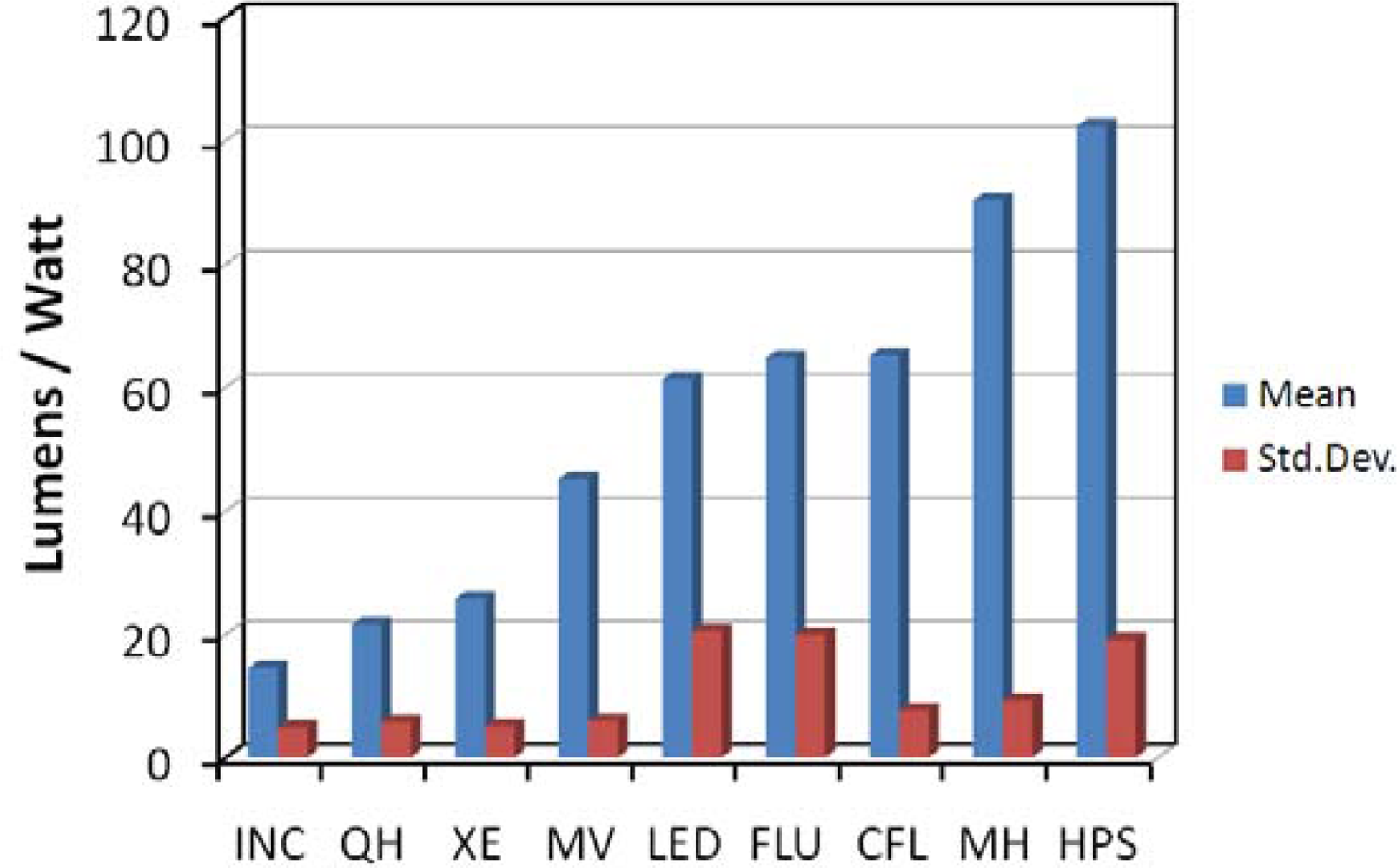
| Type | Description | CCT | CRI | Lumens | Watts | LE | |
|---|---|---|---|---|---|---|---|
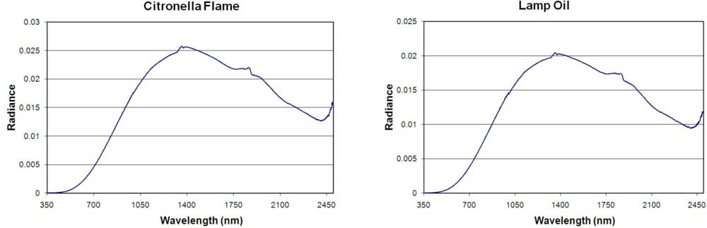
| 1 | Liquid Fuel | Citronella Oil | 1941 | 100 | |||
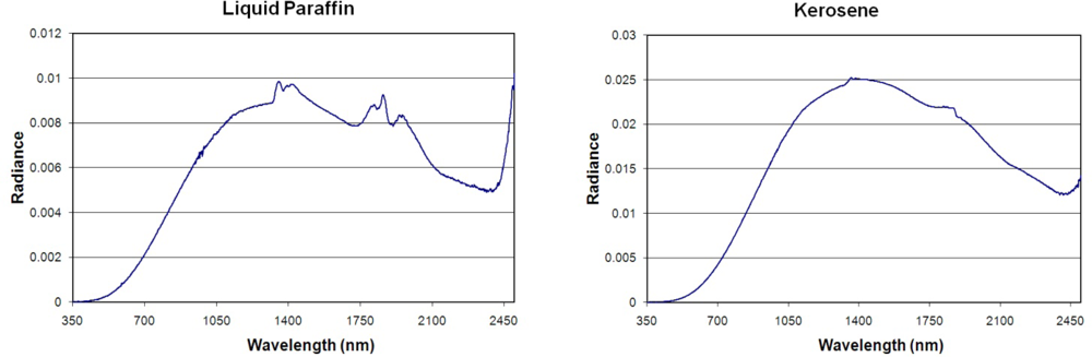
| 2 | Liquid Fuel | Kerosene | 1913 | 100 | |||
| 3 | Liquid Fuel | Lamp Oil | 1935 | 99 | |||
| 4 | Liquid Fuel | Liquid Paraffin | 2038 | 100 | |||
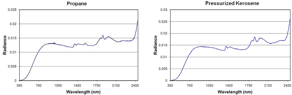
| 5 | Pressurized Fuel | Pressurized Kerosene | 2308 | 96 | |||
| 6 | Pressurized Fuel | Propane | 2380 | 100 | |||
| 7 | Incandescent | 100 Watt Spot | 2709 | 99 | |||
| 8 | Incandescent | 100 Watt Neodymium | 2604 | 73 | 960 | 100 | 9.6 |
| 9 | Incandescent | 200 Watt clear | 2826 | 100 | 3980 | 200 | 19.9 |
| 10 | Incandescent | 52 Watt frosted | 2632 | 100 | 710 | 52 | 14.0 |
| 11 | Quartz Halogen | 300 Watt double ended | 2775 | 100 | 6100 | 300 | 20.3 |
| 12 | Quartz Halogen | 60 Watt standard base | 2788 | 100 | 900 | 60 | 15.0 |
| 13 | Fluorescent | 13 Watt compact | 2886 | 81 | 900 | 13 | 69.2 |
| 14 | Fluorescent | 9 Watt compact | 2766 | 83 | 550 | 9 | 61.1 |
| 15 | Fluorescent | 4100 CCT (a) | 4009 | 79 | 2950 | 32 | 92.2 |
| 16 | Fluorescent | High CRI | 4279 | 80 | |||
| 17 | Fluorescent | Low CRI | 4415 | 5 | |||
| 18 | Fluorescent | 5000 CCT | 5193 | 76 | |||
| 19 | Fluorescent | 4100 CCT (b) | 4452 | 82 | |||
| 20 | Fluorescent | 3500 CCT | 3560 | 75 | |||
| 21 | Fluorescent | 3000 CCT | 3056 | 82 | |||
| 22 | High Pressure Sodium | 150 W | 2056 | 17 | 16000 | 170 | 94.1 |
| 23 | High Pressure Sodium | 1000 W | 2108 | 32 | 126000 | 1000 | 126.0 |
| 24 | High Pressure Sodium | 70 W | 2005 | 7 | 6300 | 70 | 90.0 |
| 25 | Low Pressure Sodium | 18 W SOX | 1807 | 1570 | 18 | 87.2 | |
| 26 | Metal Halide | 100 W | 3610 | 65 | 9000 | 100 | 90.0 |
| 27 | Metal Halide | 70 W | 3049 | 79 | 7000 | 70 | 100.0 |
| 28 | Metal Halide | 90 W (a) | 4160 | 64 | 5600 | 90 | 62.2 |
| 29 | Metal Halide | 90 W (b) | 2874 | 100 | 6200 | 90 | 68.9 |
| 30 | Mercury Vapor | Self Ballasted | 3758 | 53 | 3000 | 160 | 10.5 |
| 31 | LED | Spotlight | 5899 | 65 | 250 | 9 | 27.8 |
| 32 | LED | Streetlight (A) | 4863 | 71 | 5580 | 109 | 51.2 |
| 33 | LED | Amber Standard Base | 8357 | ||||
| 34 | LED | Green Standard Base | 7272 | ||||
| 35 | LED | Red Standard Base | 1756 | ||||
| 36 | LED | Blue Tester | 6592 | 83 | |||
| 37 | LED | Green Tester | 3124 | 72 | |||
| 38 | LED | Orange Tester | 1739 | ||||
| 39 | LED | Red Tester | 2624 | 68 | |||
| 40 | LED | White Tester | 7419 | ||||
| 41 | LED | Yellow Tester | 2038 | 99 | |||
| 42 | LED | Streetlight (Cool White) | 6273 | 100 | 3604 | 54.3 | 66.4 |
| 43 | LED | Streetlight (Warm White) | 4464 | 100 |
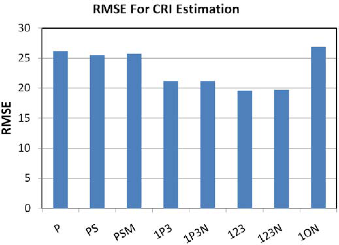
| Set 1: | Photopic (P) |
| Set 2: | Photopic, Scotopic (PS) |
| Set 3: | Photopic, Scotopic, “meltopic” (PSM) |
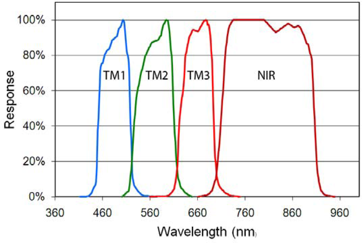
| Set 4: | TM1, Photopic, TM3 (1P3) |
| Set 5: | TM1, Photopic, TM3, NIR (1P3N) |
| Set 6: | TM1, TM2, TM3 (123) |
| Set 7: | TM1, TM2, TM3. NIR (123N) |
| Set 8: | TM1, Orange, NIR (1ON) |
© 2010 by the authors; licensee MDPI, Basel, Switzerland. This article is an open-access article distributed under the terms and conditions of the Creative Commons Attribution license ( http://creativecommons.org/licenses/by/3.0/).
Share and Cite
Elvidge, C.D.; Keith, D.M.; Tuttle, B.T.; Baugh, K.E. Spectral Identification of Lighting Type and Character. Sensors 2010, 10, 3961-3988. https://doi.org/10.3390/s100403961
Elvidge CD, Keith DM, Tuttle BT, Baugh KE. Spectral Identification of Lighting Type and Character. Sensors. 2010; 10(4):3961-3988. https://doi.org/10.3390/s100403961
Chicago/Turabian StyleElvidge, Christopher D., David M. Keith, Benjamin T. Tuttle, and Kimberly E. Baugh. 2010. "Spectral Identification of Lighting Type and Character" Sensors 10, no. 4: 3961-3988. https://doi.org/10.3390/s100403961