In this section, we first describe the confidence levels of sensor nodes to be used in the proposed event detection scheme. We then present our adaptive event detection scheme using the confidence levels defined. Some erroneous readings due to transient faults will be corrected by employing a moving average filter to further enhance event detection performance. For convenience we list the notation to be used in this paper.
3.1. Confidence Levels
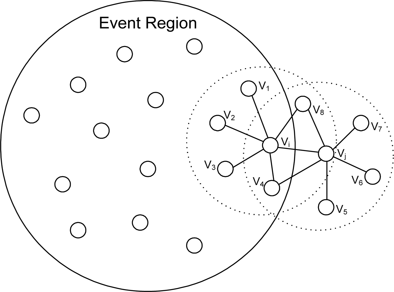
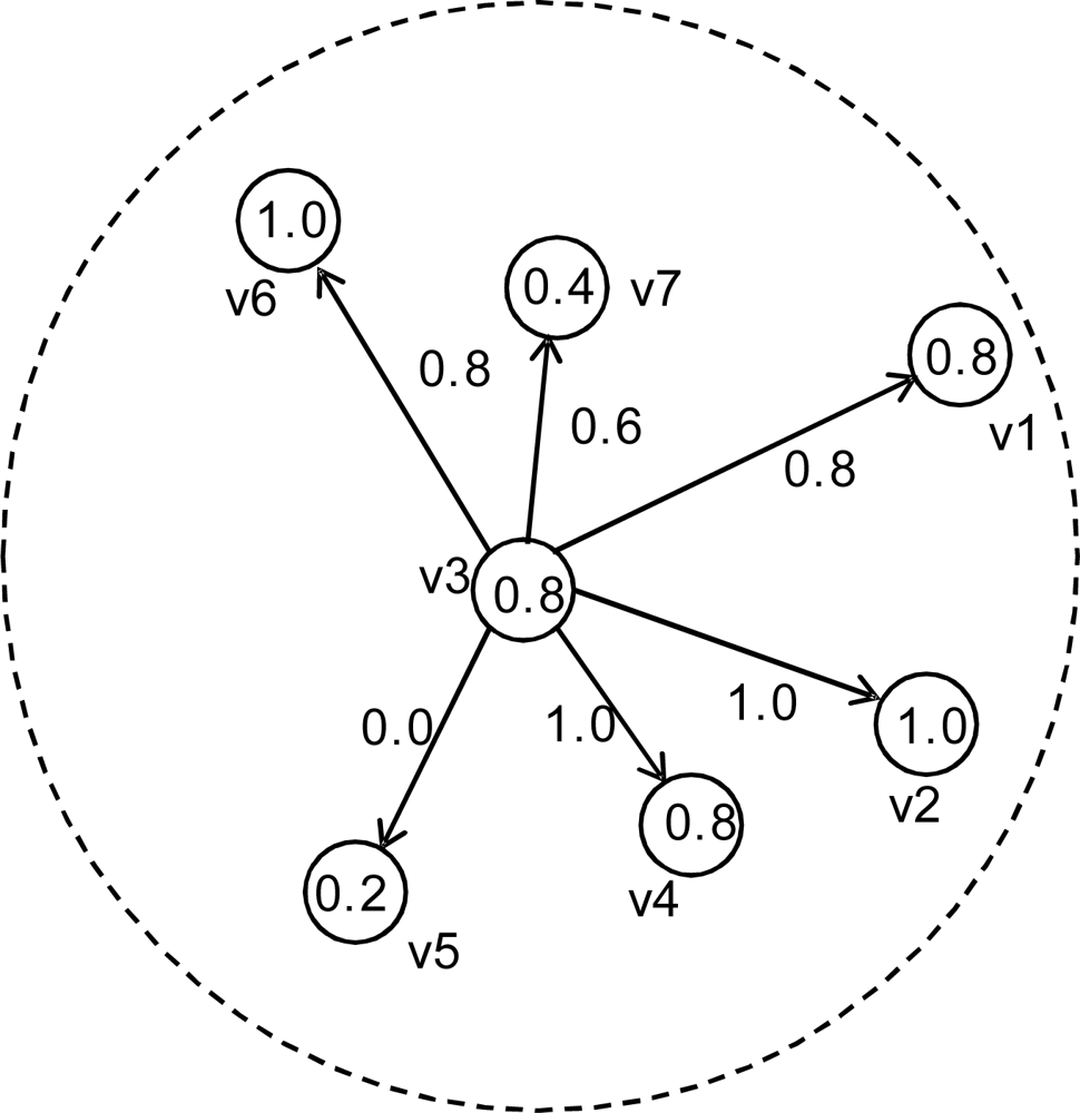
In order to describe confidence levels of a sensor node and its neighbors a sensor network is modeled here as a weighted directed graph, G(V;E), where V represents the set of sensor nodes and E represents the set of edges connecting sensor nodes. Two nodes vi and vj are said to be connected if the distance between them dist(vi, vj) is less than or equal to r (transmission range). Each node vi is assigned a self-confidence level ci. Each edge eij is also assigned a weight wij, indicating the confidence level of vj from the viewpoint of vi. The confidence levels will be used to isolate potentially faulty sensor nodes from the rest of the network. They are also used to reinstate an isolated node if the confidence levels associated with it satisfy the required conditions to be addressed shortly. We use cmin and cmax to denote the range of the confidence level ci. Also wmin and wmax will be used to indicate the range of wij.
An illustration is given in
Figure 1, where six nodes are neighbors of the node
v3 (
i.e., six nodes are located within the communication range of
v3) and confidence levels
ci and
wij are assumed to be in the range of 0 to 1. In the figure, from the viewpoint of node
v3,
v2 and
v4 are nodes with the highest confidence while
v5 is a node with the lowest confidence. Among the six neighboring nodes of
v3,
v5 is the most likely to be faulty, and will be ignored from
v3 if
wmin = 0.
The confidence levels will be updated each time a fault detection or event detection is performed. All the ci and wij are initialized to 1 (i.e., cmax and wmax). They are increased or decreased by α (0 < α < 1) when the required conditions to be explained later are met.
3.2. Filtering Transient Faults
Event detection performance will degrade as the fault probability p increases. Hence reducing the effective p is desirable to make an event detection scheme robust to faults occurring in sensor networks. In order to do that, we use the confidence levels defined above to isolate faulty nodes and employ a modified moving average filter, to be discussed here, to correct some erroneous sensor readings due to transient faults.
Let
represent sensor reading at node
vi at time
k. Then the filter we employ takes an average of the last
M readings,
,
and
, and sets the output
to 1 if it passes a given threshold
δ. Hence the output
(
i.e., filtered output at node
vi) can be expressed as follows:
Parameters, M (i.e., window size) and δ (threshold) need to be properly chosen, depending on applications, for the best performance. They can be dynamically adjusted to enhance adaptability. As long as most of erroneous readings due to transient faults can be corrected, however, a high event detection performance can be obtained as will be shown in the simulation results in Section 4. Due to the fact that an event may cause abnormal sensor readings for an extended period of time, most transient faults can be filtered unless they occur repeatedly within the window. Although the types of faults may differ depending on applications, most random transient faults can be corrected even with a small window size. The resulting reduction in effective fault probability can affect positively on event detection performance.
Table 1 shows how erroneous readings due to some transient faults are corrected when
M = 4 and
δ = 0.75. For
i = 1, the filter at node
v1 will generate 0's even if
and
are 1. In the case of
i = 5, where an event occurs at time 1 and
v5 is assumed to be in the event region, the output becomes 1 with a delay of two cycles. That is,
becomes 1.
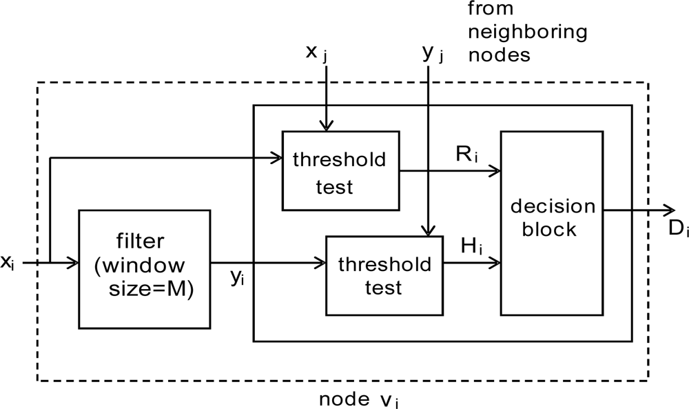
Both
x′js and
y′js will be used in event detection as shown in
Figure 2, where two identical blocks are employed to perform threshold tests (to be addressed shortly) with
x′js and
y′js, respectively. The resulting binary decisions,
Ri and
Hi, will be given to the subsequent decision block to make a final decision
Di on an event.
In the majority voting in [
2], only the upper left threshold test block is employed like most other schemes, although the block could be functionally different. In our proposed event detection scheme both
Ri and
Hi are used. The final decision
Di on an event will be made based on
Hi, while
Ri is used as a warning of an event.
3.3. Dynamic Threshold Selection
In this subsection, we present our adaptive event detection scheme, focusing on the threshold test block in
Figure 2, where the confidence levels introduced in the previous subsection will be used to dynamically adjust the threshold for event detection. The confidence levels, updated each time event detection/fault detection is performed, are utilized to isolate potentially faulty sensor nodes and reinstate them if some given conditions are met. The resulting changes are to be reflected in the number of neighboring nodes (
i.e., the effective node degree
at time
k) of each node
vi, and it will in turn modify the threshold
θ for the next event detection cycle. In order to realize this adaptivity, each sensor node
vi holds its fault status
Fi, its self-confidence level
ci, the confidence levels of its neighboring nodes
wij, and the fault status of node
vj from the viewpoint of
vi,
Fij.
The proposed event detection scheme, where the threshold θ is dynamically adjusted depending on the effective node degree, can be depicted as follows. Majority voting is used in the threshold test. Fi and Fij are initialized to 0 (good).
Adaptive Event Detection Scheme
Obtain sensor reading xi and filter it to get yi Obtain sensor readings xj, filtered outputs yj, and Fj from neighbors Set the threshold θ to di/2 Determine bi, the number of neighbors with xj = xi Determine qi, the number of neighbors with yj = yi If qi ≥ θ, then Hi ← yi, else Hi ← ¬yi If bi ≥ θ, then Ri ← xi, else Ri ← ¬xi Report an event (i.e., Di = 1) if Hi=1 Report a warning if Ri = 1 Update the confidence levels ci and wij
|
In steps 1 and 2, each sensor node receives its own and neighbors’ sensor readings (including filtered ones). Steps 3 to 5 are functions to be performed in the two threshold test blocks in
Figure 2. In step 3, the threshold value for majority voting to be used in step 5 is determined. Step 5 will set
Ri (
Hi) to either 0 or 1 depending on the number of matching neighbors obtained in step 4.
Ri and
Hi at node
vi can be set against its own readings if the node fails to pass the threshold. In step 6, the decision on an event will be made.
Ri = 1 will be taken as a warning since it might occur due to transient faults. If it is an indication of an event, the decision on an event will be made at the time
Hi becomes 1. The warning must be given to its neighboring nodes to shorten the cycle time momentarily so that an event can be reported quickly. Confidence levels are updated in step 7. The confidence level of
vj from the viewpoint of
vi,
wij, is updated according to
Table 2.
As shown in
Table 2,
wij is increased by
α only when
Fj = 0 (good) and
Di =
yj. In other words, confidence level of
vj from the viewpoint of
vi becomes higher when both
vi and
vj have similar sensor readings and
vj is currently in the good state. The second and fourth rows decrease
wij by
α since
Fj = 1 (faulty).
The third row can be explained using the following three representative cases among others. It lowers the confidence level of its neighboring node vj only when Di is equal to 0.
Case 1: Suppose that two good nodes
vi and
vj are neighboring each other and each of them is surrounded by sufficient number of good nodes to pass the threshold test. The first case occurs when
vj becomes faulty and sends a 1 as shown in
Figure 3. In this case,
vi will have
Di = 0,
yj = 1, and
Fj = 0 (until
vj sets
Fj to 1). Hence the conditions are met. The desired action at node
vi, as far as confidence level is concerned, is to lower the confidence level of
vj (
i.e.,
wij).
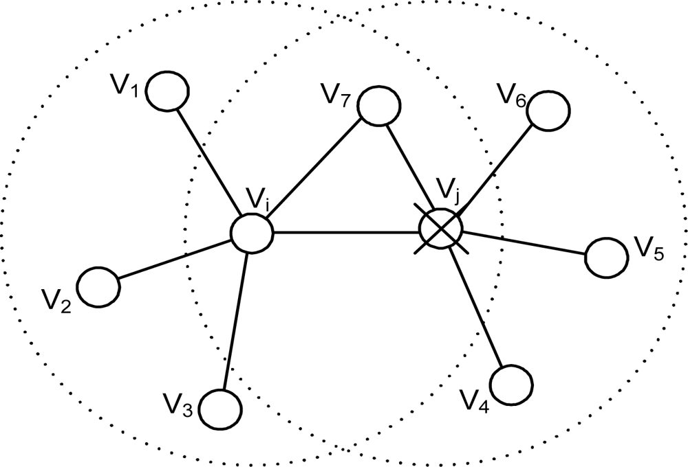
Case 2: The conditions can also be met when two good nodes,
vi and
vj, neighboring each other are located in such a way that only one of them is in the event region, as illustrated in
Figure 4. In the figure,
vi is in the event region and receives a 1 from
v1 through
v4 and will eventually report an event (
i.e.,
Di = 1). Meanwhile,
vj also makes the right decision of no-event (
i.e.,
Dj = 0). When
yi = 1 and
yj = 0, as expected,
vi will have
Di = 1,
yj = 0, and
Fj = 0, satisfying the conditions. The conditions are also met for
vj since
Dj = 0,
yi = 1, and
Fi = 0. The correct action in case 2, as far as confidence level is concerned, is as follows: (a) at node
vi,
wij needs to be increased, (b) at node
vj,
wji also needs to be increased.
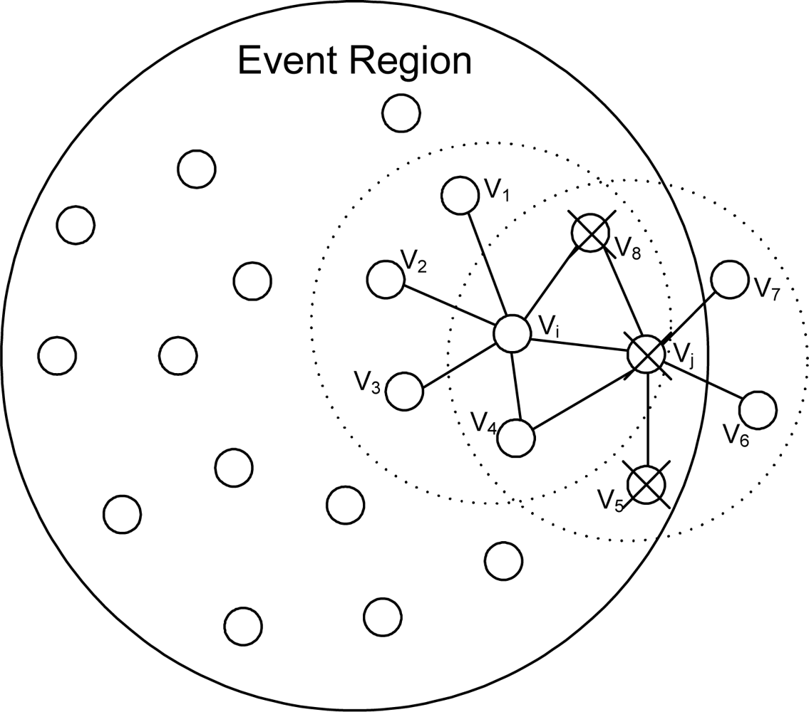
Case 3: It occurs when faulty nodes in close proximity, claiming to be good, are in an event region as shown in
Figure 5 such that their readings are 0 as opposed to 1 (abnormal). Suppose that two nodes in the event region,
vi and
vj, are neighboring each other and
vj is one of the faulty nodes. Apparently
vj may have
Dj = 0 since
v6 and
v7 are likely to report a 0 since they are outside the event region. Both
vi and
vj meet the conditions. The proper actions in this case are (a) at node
vi, where
Di = 1,
yj = 0, and
Fj = 0,
wij has to be lowered, (b) at node
vj, where
Dj = 0,
yi = 1, and
Fi = 0,
wji needs to be increased to eventually change
Fj to 1.
For node vi the above cases can be divided into two groups, depending on the value of Di. The first group (Di = 0) includes case 1, case 2(b), and case 3(b). Although the three cases in the first group cannot be distinguished based on the given information, the desired actions may differ. Only case 1 wants to lower the confidence level. The second group (Di = 1) includes case 2(a) and case 3(a), requesting conflicting actions. The third row in the table allows only case 1 to update the confidence level, ignoring all other cases. The reasons for taking this action are as follows. Confidence levels are maintained to isolated nodes with permanent faults or nodes behaving incorrectly for some extended period of time. Hence it is primarily intended to handle case 1. All other cases are related to events, which in general consume a relatively small portion of the entire monitoring time. In the case of an event, due to the conflicting requests, correctly updating confidence levels needs some additional information on the exact boundary of the event region, requiring more sophisticated computations. Hence momentarily stopping the updates in the case of an event may be appropriate since the network continues its monitoring function with most of the faulty nodes isolated.
Based on
Table 2 the confidence level
wij is updated as follows.
It is increased or decreased by α each time the conditions are met. The value of α needs to be chosen depending on the types of faults and applications. If α is relatively small, a node with transient faults is highly unlikely to be removed from the neighbor list. As α increases, however, it can be removed with an increased probability. Even if it is isolated, the node with only transient faults will be reinstated in our adaptive scheme.
A potentially faulty neighboring node vj of node vi will be removed from the effective neighbor list of vi as follows. If Fij = 0 (good) and wij = wmin, Fij is set to 1 (faulty) and vj is removed from vi’s effective neighbor list. On the other hand, if Fij = 1 (faulty) and wij = wmax, Fij will be set to 0 (good) and vj will rejoin the vi’s effective neighbor list. Once a node is removed from the list (i.e., wij = wmin), it can rejoin the list only when wij is increased and reaches wmax. Similarly, once a removed node rejoins the effective neighbor list, it will remain there unless wij reaches wmin again.
Similarly the self-confidence level of vi, ci, is also updated in step 7. It is lowered if the decision made at vi, Di, is different from its own sensor reading filtered, yi, except for an event.
Fault status Fi changes depending on the self confidence level ci. Fi will be set to 1 (faulty) when ci becomes cmin. Once it is set to 1, it will stay there until ci reaches cmax again.
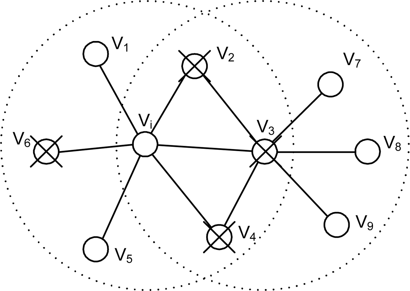
In the case where a good sensor node has more faulty neighbors, the node might be determined to be faulty, as illustrated in
Figure 6, where
ci for
vi will be lowered due to the inequality
Di ≠
yi. It, however, will highly likely be determined to be a good node with time. The node,
v3, a neighbor of
vi, will determine itself to be faulty if it cannot pass the threshold such that its confidence level
c3 reaches 0. In the figure,
v3 has more good neighbors than faulty ones. Hence
D3 is highly unlikely to be
y3. Once
F3 is set to 1,
vi will remove
v3 from its neighbor list. As a result, its effective node degree
will be lowered. If this also happens at
v4, for example, the node is also removed from the list, and the node degree of
vi is further lowered. Finally,
vi passes the threshold, changes its fault status to 0 (good) some cycles later, and it can then be treated as a good node. If a larger number of faulty nodes are in close proximity, this recovery might not happen. The case, however, is extremely unlikely since our adaptive scheme removes faulty nodes as soon as identified. Unless all the nodes become faulty almost simultaneously, such a situation is unlikely to occur.

