<?xml version="1.0" encoding="UTF-8"?>
<!DOCTYPE article PUBLIC "-//NLM//DTD Journal Publishing DTD v2.3 20070202//EN" "journalpublishing.dtd">
<article xmlns:mml="http://www.w3.org/1998/Math/MathML" xmlns:xlink="http://www.w3.org/1999/xlink" xml:lang="en" article-type="research-article">
<front>
<journal-meta>
<journal-id journal-id-type="nlm-ta">Sensors</journal-id>
<journal-title>Sensors</journal-title>
<issn pub-type="epub">1424-8220</issn>
<publisher>
<publisher-name>Molecular Diversity Preservation International (MDPI)</publisher-name></publisher></journal-meta>
<article-meta>
<article-id pub-id-type="doi">10.3390/s101211428</article-id>
<article-id pub-id-type="publisher-id">sensors-10-11428</article-id>
<article-categories>
<subj-group>
<subject>Article</subject></subj-group></article-categories>
<title-group>
<article-title>Myocardial Motion Analysis for Determination of Tei-Index of Human Heart</article-title></title-group>
<contrib-group>
<contrib contrib-type="author">
<name><surname>Chen</surname><given-names>Shengyong</given-names></name><xref ref-type="aff" rid="af1-sensors-10-11428">1</xref><xref ref-type="corresp" rid="c1-sensors-10-11428">⋆</xref></contrib>
<contrib contrib-type="author">
<name><surname>Zhang</surname><given-names>Jianhua</given-names></name><xref ref-type="aff" rid="af1-sensors-10-11428">1</xref><xref ref-type="aff" rid="af2-sensors-10-11428">2</xref><xref ref-type="corresp" rid="c1-sensors-10-11428">⋆</xref></contrib>
<contrib contrib-type="author">
<name><surname>Zhang</surname><given-names>Houxiang</given-names></name><xref ref-type="aff" rid="af2-sensors-10-11428">2</xref></contrib>
<contrib contrib-type="author">
<name><surname>Guan</surname><given-names>Qiu</given-names></name><xref ref-type="aff" rid="af1-sensors-10-11428">1</xref></contrib>
<contrib contrib-type="author">
<name><surname>Du</surname><given-names>Yahui</given-names></name><xref ref-type="aff" rid="af1-sensors-10-11428">1</xref></contrib>
<contrib contrib-type="author">
<name><surname>Yao</surname><given-names>Chunyan</given-names></name><xref ref-type="aff" rid="af1-sensors-10-11428">1</xref></contrib>
<contrib contrib-type="author">
<name><surname>Zhang</surname><given-names>Jianwei</given-names></name><xref ref-type="aff" rid="af2-sensors-10-11428">2</xref></contrib></contrib-group>
<aff id="af1-sensors-10-11428">
<label>1</label> College of Computer Science, Zhejiang University of Technology, 310023 Hangzhou, China</aff>
<aff id="af2-sensors-10-11428">
<label>2</label> Department of Informatics, University of Hamburg, 22527 Hamburg, Germany</aff>
<author-notes>
<corresp id="c1-sensors-10-11428">
<label>⋆</label>Author to whom correspondence should be addressed; E-Mails: <email>sy@ieee.org</email> (S.Y.C.); <email>jzhang@informatik.uni-hamburg.de</email> (J.H.Z.); Tel.: +8657185290525 (S.Y.C.); +4940428832361 (J.H.Z.); Fax: +8657185177103 (S.Y.C.); +4940428832397 (J.H.Z.).</corresp></author-notes>
<pub-date pub-type="collection">
<year>2010</year></pub-date>
<pub-date pub-type="epub">
<day>13</day>
<month>12</month>
<year>2010</year></pub-date>
<volume>10</volume><issue>12</issue>
<fpage>11428</fpage>
<lpage>11439</lpage>
<history>
<date date-type="received">
<day>4</day>
<month>11</month>
<year>2010</year></date>
<date date-type="rev-recd">
<day>24</day>
<month>11</month>
<year>2010</year></date>
<date date-type="accepted">
<day>8</day>
<month>12</month>
<year>2010</year></date></history>
<permissions>
<copyright-statement>© 2010 by the authors; licensee MDPI, Basel, Switzerland.</copyright-statement>
<copyright-year>2010</copyright-year>
<license>
<p>This article is an open access article distributed under the terms and conditions of the Creative Commons Attribution license (<ext-link xlink:href="http://creativecommons.org/licenses/by/3.0/" ext-link-type="uri">http://creativecommons.org/licenses/by/3.0/</ext-link>).</p></license></permissions>
<abstract>
<p>The Tei index, an important indicator of heart function, lacks a direct method to compute because it is difficult to directly evaluate the isovolumic contraction time (ICT) and isovolumic relaxation time (IRT) from which the Tei index can be obtained. In this paper, based on the proposed method of accurately measuring the cardiac cycle physical phase, a direct method of calculating the Tei index is presented. The experiments based on real heart medical images show the effectiveness of this method. Moreover, a new method of calculating left ventricular wall motion amplitude is proposed and the experiments show its satisfactory performance.</p></abstract>
<kwd-group>
<kwd>cardiac cycle physical phase</kwd>
<kwd>Tei index</kwd>
<kwd>left ventricular wall motion amplitude</kwd>
<kwd>computer vision</kwd>
<kwd>image processing</kwd></kwd-group></article-meta></front>
<body>
<sec sec-type="intro">
<label>1.</label>
<title>Introduction</title>
<p>Cardiovascular diseases have become the top factor causing human death in both western and eastern world. People hope that these diseases can be traced before they onset. A simple, reproducible, non-invasive test for determinants of prognosis is therefore necessary. For this kind of test, doctors need to observe the current status of hearts and have some effective measurement rules to decide if hearts is normal or not. For non-invasive check methods, there are several heart medical imaging technologies, such as MR, CT, SPECT and Ultrasound, widely used for heart diseases diagnosis, from which doctors can observe patients heart status without invasion.</p>
<p>Myocardial motion that is directly related to cardiac vascular supply is widely studied based on heart medical images to analyze the heart condition, especially the left ventricular function, for diagnosing heart abnormalities [<xref ref-type="bibr" rid="b1-sensors-10-11428">1</xref>–<xref ref-type="bibr" rid="b3-sensors-10-11428">3</xref>]. Left ventricular (LV) is the most important part of heart and LV function is generally analyzed to diagnose the heart condition. Traditionally, LV systolic function is used as measurement of the heart condition. However, LV diastolic function is also an important indicator of the heart condition. Both of them are important determinants of prognosis. A clinical assessment of using both LV systolic and diastolic function will be better than using only one of them. The Tei index [<xref ref-type="bibr" rid="b4-sensors-10-11428">4</xref>], raised originally by Tei in 1995, can be used to assess both LV systolic and diastolic function at the same time and consequently becomes an important indicator of heart condition [<xref ref-type="bibr" rid="b5-sensors-10-11428">5</xref>,<xref ref-type="bibr" rid="b6-sensors-10-11428">6</xref>]. In [<xref ref-type="bibr" rid="b7-sensors-10-11428">7</xref>], several literatures had been reviewed in which the Tei index had been proved to be used to diagnose many cardiovascular diseases. The Tei index can be used to assess either left or right ventricular function, calculated as the sum of the isovolumic contraction time (ICT) and isovolumic relaxation time (IRT) divided by ejection time (ET). The ICT and IRT, however, are very difficult to calculate because of the lack of the whole deform information of LV. The Tei index is therefore generally measured by indirect methods (e.g., [<xref ref-type="bibr" rid="b8-sensors-10-11428">8</xref>,<xref ref-type="bibr" rid="b9-sensors-10-11428">9</xref>]. The originally method to evaluate the time intervals is through pulsed-wave Doppler velocity spectra of ventricular inflow and outflow [<xref ref-type="bibr" rid="b4-sensors-10-11428">4</xref>]. However, there is possible error source because of the inability to acquire inflow and outflow velocity spectra during the same cardiac cycle [<xref ref-type="bibr" rid="b5-sensors-10-11428">5</xref>]. The tissue Doppler imaging is employed to measure the time intervals for computing the Tei index to avoid this kind of potential error [<xref ref-type="bibr" rid="b9-sensors-10-11428">9</xref>]. Another method using left ventricular area waveforms with acoustic quantification is also introduced to calculate the Tei index for avoiding the potential error. However, both of them are also the indirect methods.</p>
<p>In the myocardial motion analysis, the cardiac cycle is a complicated time-varying process and is generally partitioned into several phases based on time to simplify the process. According to clinical diagnosis, however, the phase should be definitely based on LV deformation and stress since the dynamics of heart is caused by that deformation. This definition is called cardiac physical phase. In this paper, a method of cardiac cycle physical phase (CPP) division according to the LV anatomy is proposed first based on B-spline represented heart model, of which the initial work [<xref ref-type="bibr" rid="b10-sensors-10-11428">10</xref>] has been presented in Robio 2010. By using the proposed method, the CPP can be accurately partitioned. Based on accurately CPP partitions, a direct method to accurately measure the Tei index is then presented by computing the ICT and IRT from CPP. To our knowledge, it is the first direct calculation of the Tei index in literatures. In particular, the SPECT heart images are used in this study. As a kind of new application of heart medical images, the proposed calculation of the Tei index is proved better than traditional assessment methods.</p>
<p>Moreover, LV wall motion amplitude (LVMA) can also be computed to analyze the LV wall movement based on the accurate CPP partitions in this study. The movement of LV wall is another very important index of the LV function [<xref ref-type="bibr" rid="b11-sensors-10-11428">11</xref>,<xref ref-type="bibr" rid="b12-sensors-10-11428">12</xref>]. It reflects the deformation capability of LV. Traditionally, the analysis of LV wall movement is focused on myocardial velocities [<xref ref-type="bibr" rid="b13-sensors-10-11428">13</xref>,<xref ref-type="bibr" rid="b14-sensors-10-11428">14</xref>]. The LVMA, however, can indicate directly the abnormal area of LV wall when there is heart disease [<xref ref-type="bibr" rid="b15-sensors-10-11428">15</xref>]. Through LVMA, the ill area of heart with abnormal amplitude could be detected and localized, which will of course improve the effect of diagnosis.</p>
<p>The organization of this paper is as follows. In the next section, the matrix representation of B-spline is introduced and the volumetric measurement of B-spline is given. The method of CPP partition and calculation of Tei and LVMA are explained in Section 3. The proposed methods are evaluated by experiments on a real human data in Section 4 and the results are also analyzed.</p></sec>
<sec>
<label>2.</label>
<title>Shape Representation for Volumetric Measurement</title>
<sec>
<label>2.1.</label>
<title>Matrix representation of B-spline</title>
<p>A B-spline curve consists of segments, with each segment of degree k constructed by k+1 sequential control points. Let <italic>t</italic> = (<italic>u</italic>–<italic>u<sub>i</sub></italic>)/(<italic>u<sub>i</sub></italic><sub>+1</sub> –<italic>u<sub>i</sub></italic>), the segment has the following matrix form [<xref ref-type="bibr" rid="b16-sensors-10-11428">16</xref>,<xref ref-type="bibr" rid="b17-sensors-10-11428">17</xref>] in the nonempty interval [<italic>u<sub>i</sub></italic>,<italic>u<sub>i</sub></italic><sub>+1</sub>]:
<disp-formula id="FD1">
<label>(1)</label>
<mml:math display="block">
<mml:mrow>
<mml:msub>
<mml:mi>p</mml:mi>
<mml:mi>i</mml:mi></mml:msub>
<mml:mo stretchy="false">(</mml:mo>
<mml:mi>t</mml:mi>
<mml:mo stretchy="false">)</mml:mo>
<mml:mo>=</mml:mo>
<mml:mrow>
<mml:mo>[</mml:mo>
<mml:mrow>
<mml:mn>1</mml:mn>
<mml:mi> </mml:mi>
<mml:mi> </mml:mi>
<mml:mi> </mml:mi>
<mml:mi> </mml:mi>
<mml:mi> </mml:mi>
<mml:mi>t</mml:mi>
<mml:mi> </mml:mi>
<mml:mi> </mml:mi>
<mml:mi> </mml:mi>
<mml:mi> </mml:mi>
<mml:mi> </mml:mi>
<mml:msup>
<mml:mi>t</mml:mi>
<mml:mn>2</mml:mn></mml:msup>
<mml:mi> </mml:mi>
<mml:mi> </mml:mi>
<mml:mi> </mml:mi>
<mml:mo>⋯</mml:mo>
<mml:mi> </mml:mi>
<mml:mi> </mml:mi>
<mml:mi> </mml:mi>
<mml:msup>
<mml:mi>t</mml:mi>
<mml:mi>k</mml:mi></mml:msup></mml:mrow>
<mml:mo>]</mml:mo></mml:mrow>
<mml:msubsup>
<mml:mi>M</mml:mi>
<mml:mi>i</mml:mi>
<mml:mrow>
<mml:mi>k</mml:mi>
<mml:mo>+</mml:mo>
<mml:mn>1</mml:mn></mml:mrow></mml:msubsup>
<mml:msup>
<mml:mrow>
<mml:mrow>
<mml:mo>[</mml:mo>
<mml:mrow>
<mml:msub>
<mml:mi>V</mml:mi>
<mml:mrow>
<mml:mi>i</mml:mi>
<mml:mo>−</mml:mo>
<mml:mi>k</mml:mi></mml:mrow></mml:msub>
<mml:mi> </mml:mi>
<mml:mi> </mml:mi>
<mml:mi> </mml:mi>
<mml:mi> </mml:mi>
<mml:mi> </mml:mi>
<mml:msub>
<mml:mi>V</mml:mi>
<mml:mrow>
<mml:mi>i</mml:mi>
<mml:mo>−</mml:mo>
<mml:mi>k</mml:mi>
<mml:mo>+</mml:mo>
<mml:mn>1</mml:mn></mml:mrow></mml:msub>
<mml:mi> </mml:mi>
<mml:mi> </mml:mi>
<mml:mi> </mml:mi>
<mml:mo>⋯</mml:mo>
<mml:mi> </mml:mi>
<mml:mi> </mml:mi>
<mml:mi> </mml:mi>
<mml:msub>
<mml:mi>V</mml:mi>
<mml:mi>i</mml:mi></mml:msub></mml:mrow>
<mml:mo>]</mml:mo></mml:mrow></mml:mrow>
<mml:mi>T</mml:mi></mml:msup></mml:mrow></mml:math></disp-formula>where <italic>t</italic> ∈ [0,1] and <italic>V</italic> is the vector of <italic>k</italic>+1 control points. The number of control points are denoted as <italic>i</italic> = <italic>k</italic>,<italic>k</italic>+1, ⋯,<italic>n</italic>+1 and the <italic>i</italic>th basis matrix, 
<inline-formula>
<mml:math>
<mml:msubsup>
<mml:mi>M</mml:mi>
<mml:mi>i</mml:mi>
<mml:mrow>
<mml:mi>k</mml:mi>
<mml:mo>+</mml:mo>
<mml:mn>1</mml:mn></mml:mrow></mml:msubsup></mml:math></inline-formula>, is the matrix form of B-spline basis in order <italic>k</italic>.</p>
<p>The whole curve can thus be represented as:
<disp-formula id="FD2">
<label>(2)</label>
<mml:math display="block">
<mml:mtable columnalign="left">
<mml:mtr>
<mml:mtd>
<mml:mi>P</mml:mi>
<mml:mo stretchy="false">(</mml:mo>
<mml:mi>t</mml:mi>
<mml:mo stretchy="false">)</mml:mo>
<mml:mo>=</mml:mo>
<mml:munderover>
<mml:mo>∑</mml:mo>
<mml:mrow>
<mml:mi>i</mml:mi>
<mml:mo>=</mml:mo>
<mml:mi>k</mml:mi></mml:mrow>
<mml:mi>n</mml:mi></mml:munderover>
<mml:mrow>
<mml:msub>
<mml:mi>p</mml:mi>
<mml:mi>i</mml:mi></mml:msub>
<mml:mo stretchy="false">(</mml:mo>
<mml:mi>t</mml:mi>
<mml:mo stretchy="false">)</mml:mo></mml:mrow>
<mml:mo>=</mml:mo>
<mml:munderover>
<mml:mo>∑</mml:mo>
<mml:mrow>
<mml:mi>i</mml:mi>
<mml:mo>=</mml:mo>
<mml:mi>k</mml:mi></mml:mrow>
<mml:mi>n</mml:mi></mml:munderover>
<mml:mrow>
<mml:munderover>
<mml:mo>∑</mml:mo>
<mml:mrow>
<mml:mi>j</mml:mi>
<mml:mo>=</mml:mo>
<mml:mn>0</mml:mn></mml:mrow>
<mml:mi>k</mml:mi></mml:munderover>
<mml:mrow>
<mml:msub>
<mml:mi>a</mml:mi>
<mml:mi>i</mml:mi></mml:msub>
<mml:mo stretchy="false">(</mml:mo>
<mml:mi>j</mml:mi>
<mml:mo stretchy="false">)</mml:mo>
<mml:msup>
<mml:mi>t</mml:mi>
<mml:mi>j</mml:mi></mml:msup></mml:mrow></mml:mrow></mml:mtd></mml:mtr>
<mml:mtr>
<mml:mtd>
<mml:mi> </mml:mi>
<mml:mi> </mml:mi>
<mml:mi> </mml:mi>
<mml:mi> </mml:mi>
<mml:mi> </mml:mi>
<mml:mi> </mml:mi>
<mml:mi> </mml:mi>
<mml:mi> </mml:mi>
<mml:mi> </mml:mi>
<mml:mi> </mml:mi>
<mml:mo>=</mml:mo>
<mml:munderover>
<mml:mo>∑</mml:mo>
<mml:mrow>
<mml:mi>i</mml:mi>
<mml:mo>=</mml:mo>
<mml:mi>k</mml:mi></mml:mrow>
<mml:mi>n</mml:mi></mml:munderover>
<mml:mrow>
<mml:munderover>
<mml:mo>∑</mml:mo>
<mml:mrow>
<mml:mi>j</mml:mi>
<mml:mo>=</mml:mo>
<mml:mn>0</mml:mn></mml:mrow>
<mml:mi>k</mml:mi></mml:munderover>
<mml:mrow>
<mml:mo stretchy="false">(</mml:mo>
<mml:munderover>
<mml:mo>∑</mml:mo>
<mml:mrow>
<mml:mi>l</mml:mi>
<mml:mo>=</mml:mo>
<mml:mn>0</mml:mn></mml:mrow>
<mml:mi>k</mml:mi></mml:munderover>
<mml:mrow>
<mml:msubsup>
<mml:mi>M</mml:mi>
<mml:mi>i</mml:mi>
<mml:mrow>
<mml:mi>k</mml:mi>
<mml:mo>+</mml:mo>
<mml:mn>1</mml:mn></mml:mrow></mml:msubsup>
<mml:mo stretchy="false">(</mml:mo>
<mml:mi>j</mml:mi>
<mml:mo>,</mml:mo>
<mml:mi> </mml:mi>
<mml:mi>l</mml:mi>
<mml:mo stretchy="false">)</mml:mo>
<mml:msub>
<mml:mi>V</mml:mi>
<mml:mrow>
<mml:mi>i</mml:mi>
<mml:mo>−</mml:mo>
<mml:mi>k</mml:mi>
<mml:mo>+</mml:mo>
<mml:mi>l</mml:mi></mml:mrow></mml:msub></mml:mrow>
<mml:mo stretchy="false">)</mml:mo>
<mml:msup>
<mml:mi>t</mml:mi>
<mml:mi>j</mml:mi></mml:msup></mml:mrow></mml:mrow></mml:mtd></mml:mtr></mml:mtable></mml:math></disp-formula>where
<disp-formula id="FD3">
<label>(3)</label>
<mml:math display="block">
<mml:msub>
<mml:mi>a</mml:mi>
<mml:mi>i</mml:mi></mml:msub>
<mml:mo stretchy="false">(</mml:mo>
<mml:mi>j</mml:mi>
<mml:mo stretchy="false">)</mml:mo>
<mml:mo>=</mml:mo>
<mml:munderover>
<mml:mo>∑</mml:mo>
<mml:mrow>
<mml:mi>l</mml:mi>
<mml:mo>=</mml:mo>
<mml:mn>0</mml:mn></mml:mrow>
<mml:mi>k</mml:mi></mml:munderover>
<mml:mrow>
<mml:msubsup>
<mml:mi>M</mml:mi>
<mml:mi>i</mml:mi>
<mml:mrow>
<mml:mi>k</mml:mi>
<mml:mo>+</mml:mo>
<mml:mn>1</mml:mn></mml:mrow></mml:msubsup></mml:mrow>
<mml:mo stretchy="false">(</mml:mo>
<mml:mi>j</mml:mi>
<mml:mo>,</mml:mo>
<mml:mi> </mml:mi>
<mml:mi>l</mml:mi>
<mml:mo stretchy="false">)</mml:mo>
<mml:msub>
<mml:mi>V</mml:mi>
<mml:mrow>
<mml:mi>i</mml:mi>
<mml:mo>−</mml:mo>
<mml:mi>k</mml:mi>
<mml:mo>+</mml:mo>
<mml:mi>l</mml:mi></mml:mrow></mml:msub></mml:math></disp-formula></p>
<p>Equally, a part of the B-spline surface in the nonempty area [<italic>u<sub>i</sub>,u<sub>i</sub></italic><sub>+1</sub>) × [<italic>v<sub>i</sub></italic>,<italic>v<sub>i</sub></italic><sub>+1</sub>) can be represented as:
<disp-formula id="FD4">
<label>(4)</label>
<mml:math display="block">
<mml:msub>
<mml:mi>s</mml:mi>
<mml:mrow>
<mml:mi>i</mml:mi>
<mml:mo>,</mml:mo>
<mml:mi>j</mml:mi></mml:mrow></mml:msub>
<mml:mo stretchy="false">(</mml:mo>
<mml:mi>t</mml:mi>
<mml:mo>,</mml:mo>
<mml:mi> </mml:mi>
<mml:mi>w</mml:mi>
<mml:mo stretchy="false">)</mml:mo>
<mml:mo>=</mml:mo>
<mml:msub>
<mml:mi>T</mml:mi>
<mml:mrow>
<mml:msub>
<mml:mi>k</mml:mi>
<mml:mn>1</mml:mn></mml:msub></mml:mrow></mml:msub>
<mml:msubsup>
<mml:mi>M</mml:mi>
<mml:mrow>
<mml:mi>i</mml:mi>
<mml:mo>,</mml:mo>
<mml:mi>u</mml:mi></mml:mrow>
<mml:mrow>
<mml:msub>
<mml:mi>k</mml:mi>
<mml:mn>1</mml:mn></mml:msub>
<mml:mo>+</mml:mo>
<mml:mn>1</mml:mn></mml:mrow></mml:msubsup>
<mml:msubsup>
<mml:mi>V</mml:mi>
<mml:mrow>
<mml:mi>i</mml:mi>
<mml:mo>,</mml:mo>
<mml:mi>j</mml:mi></mml:mrow>
<mml:mi>h</mml:mi></mml:msubsup>
<mml:msup>
<mml:mrow>
<mml:mo stretchy="false">(</mml:mo>
<mml:msubsup>
<mml:mi>M</mml:mi>
<mml:mrow>
<mml:mi>j</mml:mi>
<mml:mo>,</mml:mo>
<mml:mi>v</mml:mi></mml:mrow>
<mml:mrow>
<mml:msub>
<mml:mi>k</mml:mi>
<mml:mn>2</mml:mn></mml:msub>
<mml:mo>+</mml:mo>
<mml:mn>1</mml:mn></mml:mrow></mml:msubsup>
<mml:mo stretchy="false">)</mml:mo></mml:mrow>
<mml:mi>T</mml:mi></mml:msup>
<mml:msubsup>
<mml:mi>W</mml:mi>
<mml:mrow>
<mml:msub>
<mml:mi>k</mml:mi>
<mml:mn>2</mml:mn></mml:msub></mml:mrow>
<mml:mi>T</mml:mi></mml:msubsup></mml:math></disp-formula>where <italic>T<sub>k</sub></italic><sub><sub>1</sub></sub> = [1 <italic>t t</italic><sup>2</sup> ⋯ <italic>t</italic><sup><italic>k</italic><sub>1</sub></sup>] and 
<inline-formula>
<mml:math>
<mml:msubsup>
<mml:mi>W</mml:mi>
<mml:mrow>
<mml:msub>
<mml:mi>k</mml:mi>
<mml:mn>2</mml:mn></mml:msub></mml:mrow>
<mml:mi>T</mml:mi></mml:msubsup>
<mml:mo>=</mml:mo>
<mml:msup>
<mml:mrow>
<mml:mo>[</mml:mo>
<mml:mrow>
<mml:mn>1</mml:mn>
<mml:mi> </mml:mi>
<mml:mi> </mml:mi>
<mml:mi> </mml:mi>
<mml:mi> </mml:mi>
<mml:mi> </mml:mi>
<mml:mi>w</mml:mi>
<mml:mi> </mml:mi>
<mml:mi> </mml:mi>
<mml:mi> </mml:mi>
<mml:mi> </mml:mi>
<mml:mi> </mml:mi>
<mml:msup>
<mml:mi>w</mml:mi>
<mml:mn>2</mml:mn></mml:msup>
<mml:mi> </mml:mi>
<mml:mi> </mml:mi>
<mml:mi> </mml:mi>
<mml:mo>⋯</mml:mo>
<mml:mi> </mml:mi>
<mml:mi> </mml:mi>
<mml:mi> </mml:mi>
<mml:msup>
<mml:mi>w</mml:mi>
<mml:mrow>
<mml:msub>
<mml:mi>k</mml:mi>
<mml:mn>2</mml:mn></mml:msub></mml:mrow></mml:msup></mml:mrow>
<mml:mo>]</mml:mo></mml:mrow>
<mml:mi>T</mml:mi></mml:msup></mml:math></inline-formula> with <italic>t</italic> = (<italic>u</italic>–<italic>u<sub>i</sub></italic>)/(<italic>u<sub>i</sub></italic><sub>+1</sub> –<italic>u<sub>i</sub></italic>) and <italic>w</italic> = (<italic>v</italic>–<italic>v<sub>i</sub></italic>)/(<italic>v<sub>i</sub></italic><sub>+1</sub> –<italic>v<sub>i</sub></italic>), where <italic>u</italic>,<italic>v</italic> ∈ [<italic>u<sub>i</sub></italic>,<italic>u<sub>i</sub></italic><sub>+1</sub>) × [<italic>v<sub>i</sub></italic>,<italic>v<sub>i</sub></italic><sub>+1</sub>). 
<inline-formula>
<mml:math>
<mml:msubsup>
<mml:mi>M</mml:mi>
<mml:mrow>
<mml:mi>i</mml:mi>
<mml:mo>,</mml:mo>
<mml:mi>u</mml:mi></mml:mrow>
<mml:mrow>
<mml:msub>
<mml:mi>k</mml:mi>
<mml:mn>1</mml:mn></mml:msub>
<mml:mo>+</mml:mo>
<mml:mn>1</mml:mn></mml:mrow></mml:msubsup></mml:math></inline-formula> and 
<inline-formula>
<mml:math>
<mml:msubsup>
<mml:mi>M</mml:mi>
<mml:mrow>
<mml:mi>j</mml:mi>
<mml:mo>,</mml:mo>
<mml:mi>v</mml:mi></mml:mrow>
<mml:mrow>
<mml:msub>
<mml:mi>k</mml:mi>
<mml:mn>2</mml:mn></mml:msub>
<mml:mo>+</mml:mo>
<mml:mn>1</mml:mn></mml:mrow></mml:msubsup></mml:math></inline-formula> are the <italic>i</italic>th and <italic>j</italic>th basis matrixes in [<italic>u<sub>i</sub></italic>,<italic>u<sub>i</sub></italic><sub>+1</sub>) and [<italic>v<sub>i</sub></italic>,<italic>v<sub>i</sub></italic><sub>+1</sub>), respectively.</p>
<p>The whole surface is then represented as follow:</p>
<disp-formula id="FD5">
<label>(5)</label>
<mml:math display="block">
<mml:mtable columnalign="left">
<mml:mtr>
<mml:mtd>
<mml:mi>X</mml:mi>
<mml:mo stretchy="false">(</mml:mo>
<mml:mi>t</mml:mi>
<mml:mo>,</mml:mo>
<mml:mi> </mml:mi>
<mml:mi>w</mml:mi>
<mml:mo stretchy="false">)</mml:mo>
<mml:mo>=</mml:mo>
<mml:munderover>
<mml:mo>∑</mml:mo>
<mml:mrow>
<mml:mi>i</mml:mi>
<mml:mo>=</mml:mo>
<mml:msub>
<mml:mi>k</mml:mi>
<mml:mn>1</mml:mn></mml:msub></mml:mrow>
<mml:mi>m</mml:mi></mml:munderover>
<mml:mrow>
<mml:munderover>
<mml:mo>∑</mml:mo>
<mml:mrow>
<mml:mi>j</mml:mi>
<mml:mo>=</mml:mo>
<mml:msub>
<mml:mi>k</mml:mi>
<mml:mn>2</mml:mn></mml:msub></mml:mrow>
<mml:mi>n</mml:mi></mml:munderover>
<mml:mrow>
<mml:munderover>
<mml:mo>∑</mml:mo>
<mml:mrow>
<mml:mi>l</mml:mi>
<mml:mo>=</mml:mo>
<mml:mn>0</mml:mn></mml:mrow>
<mml:mrow>
<mml:msub>
<mml:mi>k</mml:mi>
<mml:mn>2</mml:mn></mml:msub></mml:mrow></mml:munderover>
<mml:mrow>
<mml:munderover>
<mml:mo>∑</mml:mo>
<mml:mrow>
<mml:mi>r</mml:mi>
<mml:mo>=</mml:mo>
<mml:mn>0</mml:mn></mml:mrow>
<mml:mrow>
<mml:msub>
<mml:mi>k</mml:mi>
<mml:mn>1</mml:mn></mml:msub></mml:mrow></mml:munderover>
<mml:mrow>
<mml:msubsup>
<mml:mi>B</mml:mi>
<mml:mrow>
<mml:mi>i</mml:mi>
<mml:mo>,</mml:mo>
<mml:mi>j</mml:mi></mml:mrow>
<mml:mi>x</mml:mi></mml:msubsup>
<mml:mo stretchy="false">(</mml:mo>
<mml:mi>r</mml:mi>
<mml:mo>,</mml:mo>
<mml:mi> </mml:mi>
<mml:mi>l</mml:mi>
<mml:mo stretchy="false">)</mml:mo>
<mml:msub>
<mml:mi>t</mml:mi>
<mml:mi>r</mml:mi></mml:msub>
<mml:msub>
<mml:mi>w</mml:mi>
<mml:mi>l</mml:mi></mml:msub></mml:mrow></mml:mrow></mml:mrow></mml:mrow></mml:mtd></mml:mtr>
<mml:mtr>
<mml:mtd>
<mml:mi>Y</mml:mi>
<mml:mo stretchy="false">(</mml:mo>
<mml:mi>t</mml:mi>
<mml:mo>,</mml:mo>
<mml:mi> </mml:mi>
<mml:mi>w</mml:mi>
<mml:mo stretchy="false">)</mml:mo>
<mml:mo>=</mml:mo>
<mml:munderover>
<mml:mo>∑</mml:mo>
<mml:mrow>
<mml:mi>i</mml:mi>
<mml:mo>=</mml:mo>
<mml:msub>
<mml:mi>k</mml:mi>
<mml:mn>1</mml:mn></mml:msub></mml:mrow>
<mml:mi>m</mml:mi></mml:munderover>
<mml:mrow>
<mml:munderover>
<mml:mo>∑</mml:mo>
<mml:mrow>
<mml:mi>j</mml:mi>
<mml:mo>=</mml:mo>
<mml:msub>
<mml:mi>k</mml:mi>
<mml:mn>2</mml:mn></mml:msub></mml:mrow>
<mml:mi>n</mml:mi></mml:munderover>
<mml:mrow>
<mml:munderover>
<mml:mo>∑</mml:mo>
<mml:mrow>
<mml:mi>l</mml:mi>
<mml:mo>=</mml:mo>
<mml:mn>0</mml:mn></mml:mrow>
<mml:mrow>
<mml:msub>
<mml:mi>k</mml:mi>
<mml:mn>2</mml:mn></mml:msub></mml:mrow></mml:munderover>
<mml:mrow>
<mml:munderover>
<mml:mo>∑</mml:mo>
<mml:mrow>
<mml:mi>r</mml:mi>
<mml:mo>=</mml:mo>
<mml:mn>0</mml:mn></mml:mrow>
<mml:mrow>
<mml:msub>
<mml:mi>k</mml:mi>
<mml:mn>1</mml:mn></mml:msub></mml:mrow></mml:munderover>
<mml:mrow>
<mml:msubsup>
<mml:mi>B</mml:mi>
<mml:mrow>
<mml:mi>i</mml:mi>
<mml:mo>,</mml:mo>
<mml:mi>j</mml:mi></mml:mrow>
<mml:mi>y</mml:mi></mml:msubsup>
<mml:mo stretchy="false">(</mml:mo>
<mml:mi>r</mml:mi>
<mml:mo>,</mml:mo>
<mml:mi> </mml:mi>
<mml:mi>l</mml:mi>
<mml:mo stretchy="false">)</mml:mo>
<mml:msub>
<mml:mi>t</mml:mi>
<mml:mi>r</mml:mi></mml:msub>
<mml:msub>
<mml:mi>w</mml:mi>
<mml:mi>l</mml:mi></mml:msub></mml:mrow></mml:mrow></mml:mrow></mml:mrow></mml:mtd></mml:mtr>
<mml:mtr>
<mml:mtd>
<mml:mi>Z</mml:mi>
<mml:mo stretchy="false">(</mml:mo>
<mml:mi>t</mml:mi>
<mml:mo>,</mml:mo>
<mml:mi> </mml:mi>
<mml:mi>w</mml:mi>
<mml:mo stretchy="false">)</mml:mo>
<mml:mo>=</mml:mo>
<mml:munderover>
<mml:mo>∑</mml:mo>
<mml:mrow>
<mml:mi>i</mml:mi>
<mml:mo>=</mml:mo>
<mml:msub>
<mml:mi>k</mml:mi>
<mml:mn>1</mml:mn></mml:msub></mml:mrow>
<mml:mi>m</mml:mi></mml:munderover>
<mml:mrow>
<mml:munderover>
<mml:mo>∑</mml:mo>
<mml:mrow>
<mml:mi>j</mml:mi>
<mml:mo>=</mml:mo>
<mml:msub>
<mml:mi>k</mml:mi>
<mml:mn>2</mml:mn></mml:msub></mml:mrow>
<mml:mi>n</mml:mi></mml:munderover>
<mml:mrow>
<mml:munderover>
<mml:mo>∑</mml:mo>
<mml:mrow>
<mml:mi>l</mml:mi>
<mml:mo>=</mml:mo>
<mml:mn>0</mml:mn></mml:mrow>
<mml:mrow>
<mml:msub>
<mml:mi>k</mml:mi>
<mml:mn>2</mml:mn></mml:msub></mml:mrow></mml:munderover>
<mml:mrow>
<mml:munderover>
<mml:mo>∑</mml:mo>
<mml:mrow>
<mml:mi>r</mml:mi>
<mml:mo>=</mml:mo>
<mml:mn>0</mml:mn></mml:mrow>
<mml:mrow>
<mml:msub>
<mml:mi>k</mml:mi>
<mml:mn>1</mml:mn></mml:msub></mml:mrow></mml:munderover>
<mml:mrow>
<mml:msubsup>
<mml:mi>B</mml:mi>
<mml:mrow>
<mml:mi>i</mml:mi>
<mml:mo>,</mml:mo>
<mml:mi>j</mml:mi></mml:mrow>
<mml:mi>z</mml:mi></mml:msubsup>
<mml:mo stretchy="false">(</mml:mo>
<mml:mi>r</mml:mi>
<mml:mo>,</mml:mo>
<mml:mi> </mml:mi>
<mml:mi>l</mml:mi>
<mml:mo stretchy="false">)</mml:mo>
<mml:msub>
<mml:mi>t</mml:mi>
<mml:mi>r</mml:mi></mml:msub>
<mml:msub>
<mml:mi>w</mml:mi>
<mml:mi>l</mml:mi></mml:msub></mml:mrow></mml:mrow></mml:mrow></mml:mrow></mml:mtd></mml:mtr></mml:mtable></mml:math></disp-formula></sec>
<sec>
<label>2.2.</label>
<title>Volumetric measurement</title>
<p>The volume can be expressed as [<xref ref-type="bibr" rid="b18-sensors-10-11428">18</xref>]:
<disp-formula id="FD6">
<label>(6)</label>
<mml:math display="block">
<mml:mi>V</mml:mi>
<mml:mo>=</mml:mo>
<mml:mrow>
<mml:msubsup>
<mml:mo>∫</mml:mo>
<mml:mrow>
<mml:msub>
<mml:mi>z</mml:mi>
<mml:mn>1</mml:mn></mml:msub></mml:mrow>
<mml:mrow>
<mml:msub>
<mml:mi>z</mml:mi>
<mml:mn>2</mml:mn></mml:msub></mml:mrow></mml:msubsup>
<mml:mrow>
<mml:mi>A</mml:mi>
<mml:mo stretchy="false">(</mml:mo>
<mml:mi>Z</mml:mi>
<mml:mo stretchy="false">)</mml:mo>
<mml:mi>d</mml:mi>
<mml:mi>z</mml:mi></mml:mrow></mml:mrow></mml:math></disp-formula>where <italic>A</italic>(<italic>z</italic>) is the area of the slice at depth <italic>z</italic>.</p>
<p>As the equations given by <xref ref-type="disp-formula" rid="FD1">Equation 1</xref> to <xref ref-type="disp-formula" rid="FD4">Equation 4</xref>, let 
<inline-formula>
<mml:math>
<mml:mfrac>
<mml:mrow>
<mml:mo>∂</mml:mo>
<mml:mi>S</mml:mi>
<mml:mo stretchy="false">(</mml:mo>
<mml:mi>t</mml:mi>
<mml:mo>,</mml:mo>
<mml:mi> </mml:mi>
<mml:mi>w</mml:mi>
<mml:mo stretchy="false">)</mml:mo></mml:mrow>
<mml:mrow>
<mml:mo>∂</mml:mo>
<mml:mi>t</mml:mi></mml:mrow></mml:mfrac></mml:math></inline-formula> and 
<inline-formula>
<mml:math>
<mml:mfrac>
<mml:mrow>
<mml:mo>∂</mml:mo>
<mml:mi>S</mml:mi>
<mml:mo stretchy="false">(</mml:mo>
<mml:mi>t</mml:mi>
<mml:mo>,</mml:mo>
<mml:mi> </mml:mi>
<mml:mi>w</mml:mi>
<mml:mo stretchy="false">)</mml:mo></mml:mrow>
<mml:mrow>
<mml:mo>∂</mml:mo>
<mml:mi>w</mml:mi></mml:mrow></mml:mfrac></mml:math></inline-formula> denote the derivatives of <italic>S</italic>(<italic>u</italic>,<italic>v</italic>) with respect to <italic>t</italic> and <italic>w</italic>.</p>
<p>The computation of the area of a slice at depth <italic>z</italic> is:
<disp-formula id="FD7">
<label>(7)</label>
<mml:math display="block">
<mml:mi>A</mml:mi>
<mml:mo stretchy="false">(</mml:mo>
<mml:mi>z</mml:mi>
<mml:mo stretchy="false">(</mml:mo>
<mml:mi>w</mml:mi>
<mml:mo stretchy="false">)</mml:mo>
<mml:mo>=</mml:mo>
<mml:munderover>
<mml:mo>∑</mml:mo>
<mml:mrow>
<mml:mi>j</mml:mi>
<mml:mo>=</mml:mo>
<mml:msub>
<mml:mi>k</mml:mi>
<mml:mn>2</mml:mn></mml:msub></mml:mrow>
<mml:mi>n</mml:mi></mml:munderover>
<mml:mrow>
<mml:mrow>
<mml:msubsup>
<mml:mo>∫</mml:mo>
<mml:mn>0</mml:mn>
<mml:mn>1</mml:mn></mml:msubsup>
<mml:mrow>
<mml:mi>Y</mml:mi>
<mml:mo stretchy="false">(</mml:mo>
<mml:mi>t</mml:mi>
<mml:mo>,</mml:mo>
<mml:mi> </mml:mi>
<mml:mi>w</mml:mi>
<mml:mo stretchy="false">)</mml:mo></mml:mrow></mml:mrow></mml:mrow>
<mml:mo>×</mml:mo>
<mml:mfrac>
<mml:mrow>
<mml:mo>∂</mml:mo>
<mml:mi>X</mml:mi>
<mml:mo stretchy="false">(</mml:mo>
<mml:mi>t</mml:mi>
<mml:mo>,</mml:mo>
<mml:mi> </mml:mi>
<mml:mi>w</mml:mi>
<mml:mo stretchy="false">)</mml:mo></mml:mrow>
<mml:mrow>
<mml:mo>∂</mml:mo>
<mml:mi>t</mml:mi></mml:mrow></mml:mfrac>
<mml:mi>d</mml:mi>
<mml:mi>t</mml:mi></mml:math></disp-formula>where <italic>Y</italic>(<italic>t</italic>,<italic>w</italic>) is given by <xref ref-type="disp-formula" rid="FD6">Equation 6</xref>, and 
<inline-formula>
<mml:math>
<mml:mfrac>
<mml:mrow>
<mml:mo>∂</mml:mo>
<mml:mi>X</mml:mi>
<mml:mo stretchy="false">(</mml:mo>
<mml:mi>t</mml:mi>
<mml:mo>,</mml:mo>
<mml:mi> </mml:mi>
<mml:mi>w</mml:mi>
<mml:mo stretchy="false">)</mml:mo></mml:mrow>
<mml:mrow>
<mml:mo>∂</mml:mo>
<mml:mi>t</mml:mi></mml:mrow></mml:mfrac></mml:math></inline-formula> is the derivative with respect to <italic>t</italic> and 
<inline-formula>
<mml:math>
<mml:mfrac>
<mml:mrow>
<mml:mo>∂</mml:mo>
<mml:mi>Z</mml:mi>
<mml:mo stretchy="false">(</mml:mo>
<mml:mi>t</mml:mi>
<mml:mo>,</mml:mo>
<mml:mi> </mml:mi>
<mml:mi>w</mml:mi>
<mml:mo stretchy="false">)</mml:mo></mml:mrow>
<mml:mrow>
<mml:mo>∂</mml:mo>
<mml:mi>w</mml:mi></mml:mrow></mml:mfrac></mml:math></inline-formula> is the derivative with respect to <italic>w</italic>.</p>
<p>The volume of B-spline surface of orders <italic>k</italic><sub>1</sub> × <italic>k</italic><sub>2</sub> is:
<disp-formula id="FD8">
<label>(8)</label>
<mml:math display="block">
<mml:mi>V</mml:mi>
<mml:mo>=</mml:mo>
<mml:munderover>
<mml:mo>∑</mml:mo>
<mml:mrow>
<mml:mi>i</mml:mi>
<mml:mo>=</mml:mo>
<mml:msub>
<mml:mi>k</mml:mi>
<mml:mn>1</mml:mn></mml:msub></mml:mrow>
<mml:mi>m</mml:mi></mml:munderover>
<mml:mrow>
<mml:munderover>
<mml:mo>∑</mml:mo>
<mml:mrow>
<mml:mi>j</mml:mi>
<mml:mo>=</mml:mo>
<mml:msub>
<mml:mi>k</mml:mi>
<mml:mn>2</mml:mn></mml:msub></mml:mrow>
<mml:mi>n</mml:mi></mml:munderover>
<mml:mrow>
<mml:mo stretchy="false">(</mml:mo>
<mml:munderover>
<mml:mo>∑</mml:mo>
<mml:mrow>
<mml:msub>
<mml:mi>l</mml:mi>
<mml:mn>1</mml:mn></mml:msub>
<mml:mo>=</mml:mo>
<mml:mn>1</mml:mn></mml:mrow>
<mml:mrow>
<mml:mo stretchy="false">(</mml:mo>
<mml:mn>3</mml:mn>
<mml:mo>×</mml:mo>
<mml:msub>
<mml:mi>k</mml:mi>
<mml:mn>2</mml:mn></mml:msub>
<mml:mo>−</mml:mo>
<mml:mn>1</mml:mn>
<mml:mo stretchy="false">)</mml:mo></mml:mrow></mml:munderover>
<mml:mrow>
<mml:munderover>
<mml:mo>∑</mml:mo>
<mml:mrow>
<mml:msub>
<mml:mi>l</mml:mi>
<mml:mn>2</mml:mn></mml:msub>
<mml:mo>=</mml:mo>
<mml:mn>1</mml:mn></mml:mrow>
<mml:mrow>
<mml:mo stretchy="false">(</mml:mo>
<mml:mn>3</mml:mn>
<mml:mo>×</mml:mo>
<mml:msub>
<mml:mi>k</mml:mi>
<mml:mn>1</mml:mn></mml:msub>
<mml:mo>−</mml:mo>
<mml:mn>1</mml:mn>
<mml:mo stretchy="false">)</mml:mo></mml:mrow></mml:munderover>
<mml:mrow>
<mml:msub>
<mml:mi>C</mml:mi>
<mml:mrow>
<mml:mi>i</mml:mi>
<mml:mo>,</mml:mo>
<mml:mi>j</mml:mi></mml:mrow></mml:msub>
<mml:mo stretchy="false">(</mml:mo>
<mml:msub>
<mml:mi>l</mml:mi>
<mml:mn>1</mml:mn></mml:msub>
<mml:mo>,</mml:mo>
<mml:mi> </mml:mi>
<mml:msub>
<mml:mi>l</mml:mi>
<mml:mn>2</mml:mn></mml:msub>
<mml:mo stretchy="false">)</mml:mo>
<mml:mo>×</mml:mo>
<mml:mfrac>
<mml:mn>1</mml:mn>
<mml:mrow>
<mml:msub>
<mml:mi>l</mml:mi>
<mml:mn>2</mml:mn></mml:msub>
<mml:mo>+</mml:mo>
<mml:mn>1</mml:mn></mml:mrow></mml:mfrac>
<mml:mo>×</mml:mo>
<mml:mfrac>
<mml:mn>1</mml:mn>
<mml:mrow>
<mml:msub>
<mml:mi>l</mml:mi>
<mml:mn>1</mml:mn></mml:msub>
<mml:mo>+</mml:mo>
<mml:mn>1</mml:mn></mml:mrow></mml:mfrac></mml:mrow></mml:mrow>
<mml:mo stretchy="false">)</mml:mo></mml:mrow></mml:mrow></mml:math></disp-formula>where <italic>C<sub>i</sub></italic><sub>,</sub> <italic><sub>j</sub></italic> is the matrix of size 3<italic>k</italic><sub>1</sub> × 3<italic>k</italic><sub>2</sub> which is the product of the three polynomials <italic>Y</italic>(<italic>t</italic>,<italic>w</italic>).</p></sec></sec>
<sec>
<label>3.</label>
<title>CPP Partition</title>
<sec>
<label>3.1.</label>
<title>CPP Partition</title>
<p>Cardiac cycle is a very complicated physical process. Traditional researches used to divide the cycle into two major parts as systole and diastole. During systole, LV contracts thus the blood in LV can be ejected out. On the opposite, during diastole LV bulges and imbibes blood in. The function of heart is achieved by the repeatedly alternating systole and diastole. As the LV motion is not uniform neither in systole nor in diastole, this rough partition can hardly express the true feature of LV motion. In fact it is shown by anatomy knowledge that the whole cardiac cycle contains 7 CPPs based on different LV shape and function. These CPPs are Isovolumic Systolic (IS), Rapid Ejection Period (REP), Slow Down Ejection Period (SDEP), Isovolumic Relaxation Period (IRP), Rapid Filling Period (RFP), Slow Down Filling Period (SDFP) and Atrial Systole (AS) [<xref ref-type="bibr" rid="b19-sensors-10-11428">19</xref>] where IS, REP and SDEP compose the systole and IPR, RFP, SDFP belong to the diastole.</p>
<p>The shape of LV shows various features in different CPP, and the changing of these shapes is the main basis of CPP partition. To divide the CPP phases, two shape factors are necessary. The first shape factor is the volume of LV (LVV). Assume that the LVV curve during whole cardiac cycle is already known and denoted with <italic>C</italic>(<italic>t</italic>). It is easy to understand that during the whole systole <italic>C</italic>(<italic>t</italic>) keeps decreasing, while in diastole it keeps increasing. Let curve <italic>C</italic>′(<italic>t</italic>) denote derivative of <italic>C</italic>(<italic>t</italic>). According to medical knowledge, the features of <italic>C</italic>(<italic>t</italic>) and <italic>C</italic>′(<italic>t</italic>) in each CPP can be listed as in the columns 3–4 of <xref ref-type="table" rid="t1-sensors-10-11428">Table 1</xref>. During the IS, IRP and AS phases, the values of <italic>C</italic>(<italic>t</italic>) remain almost invariant and consequently its derivative is approximate to zero. During the REP and SDEP phases, the values of <italic>C</italic>(<italic>t</italic>) keep on reducing and <italic>C</italic>′(<italic>t</italic>) is of course negative. During the RFP and SDFP phases, the values of <italic>C</italic>(<italic>t</italic>) keep on increasing and <italic>C</italic>′(<italic>t</italic>) is positive. The IS and AS, REP and SDEP, RFP and SDFP, however, are the adjacent phases, therefore it is difficult to separate them.</p>
<p>
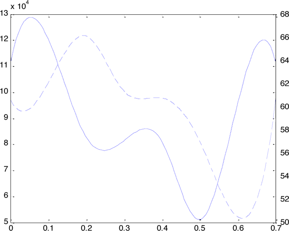
Fortunately, there is another shape factor, called LV long-axis length (LVLL), that can provide the complement information. LVLL is defined as the height from the base to the apical of LV. Assuming the LVLL curve is <italic>L</italic>(<italic>t</italic>), and its derivative is <italic>L</italic>′(<italic>t</italic>). According to the anatomy priori knowledge the <italic>L</italic>(<italic>t</italic>) and <italic>L</italic>′(<italic>t</italic>) features in each CPP are listed in the columns 5–6 of <xref ref-type="table" rid="t1-sensors-10-11428">Table 1</xref>. During IS and SDFP phases, <italic>L</italic>(<italic>t</italic>) keeps on decreasing and <italic>L</italic>′(<italic>t</italic>) is negative. During SDEP phase, <italic>L</italic>(<italic>t</italic>) keeps on increasing and <italic>L</italic>′(<italic>t</italic>) is positive. By compounding the shape factors, LVV and LVLL, it is now easy to divide the seven phases of cardiac cycle. <xref ref-type="fig" rid="f2-sensors-10-11428">Figure 2</xref> illustrate examples of <italic>C</italic>′(<italic>t</italic>) and <italic>L</italic>′(<italic>t</italic>).</p></sec>
<sec>
<label>3.2.</label>
<title>Determination of Tei index</title>
<p>In the beginning of systole and diastole, the shape of LV sharply changes while the LVV stays invariant. These periods are called isovolumetric contraction (IC) and isovolumetric relaxation (IR). Medical research shows that the biggest stress and displacement of LV occur in these two periods. When some diseases occur, the LV would need longer time to achieve the deformation and displacement, thus the length of IC and IR are very important index for evaluating LV functions. Based on that Tei-index is raised by Japanese researcher Tei in 1995 [<xref ref-type="bibr" rid="b4-sensors-10-11428">4</xref>]. The definition of Tei is:</p>
<disp-formula id="FD9">
<label>(9)</label>
<mml:math display="block">
<mml:mtext mathvariant="italic">Tei</mml:mtext>
<mml:mi> </mml:mi>
<mml:mtext mathvariant="italic">index</mml:mtext>
<mml:mo>=</mml:mo>
<mml:mfrac>
<mml:mrow>
<mml:msub>
<mml:mi>t</mml:mi>
<mml:mrow>
<mml:mi>I</mml:mi>
<mml:mi>C</mml:mi></mml:mrow></mml:msub>
<mml:mo>+</mml:mo>
<mml:msub>
<mml:mi>t</mml:mi>
<mml:mrow>
<mml:mi>I</mml:mi>
<mml:mi>R</mml:mi></mml:mrow></mml:msub></mml:mrow>
<mml:mrow>
<mml:msub>
<mml:mi>t</mml:mi>
<mml:mi>E</mml:mi></mml:msub></mml:mrow></mml:mfrac></mml:math></disp-formula>
<p>Tei index is also called myocardial performance index (MPI). This new index can generally evaluate the heart function in both diastole and systole. It has been widely used in heart disease diagnosis. Based on the CPP partition, a direct method of calculating Tei index can be deduced.</p>
<p>IC and IR are the periods while the LV shape changes largely and LVV keeps almost invariant. According to the CPP characters listed in <xref ref-type="table" rid="t1-sensors-10-11428">Table 1</xref>, it is obvious that IC is equal to IS and IR is equal to IRP. The ET is the length of systole which equals to the sum of IS, REP and SDEP.</p>
<p>The Tei index can therefore be calculated as:
<disp-formula id="FD10">
<label>(10)</label>
<mml:math display="block">
<mml:mtext mathvariant="italic">Tei</mml:mtext>
<mml:mi> </mml:mi>
<mml:mtext mathvariant="italic">index</mml:mtext>
<mml:mo>=</mml:mo>
<mml:mfrac>
<mml:mrow>
<mml:msub>
<mml:mi>t</mml:mi>
<mml:mrow>
<mml:mi>I</mml:mi>
<mml:mi>S</mml:mi></mml:mrow></mml:msub>
<mml:mo>+</mml:mo>
<mml:msub>
<mml:mi>t</mml:mi>
<mml:mrow>
<mml:mi>I</mml:mi>
<mml:mi>R</mml:mi>
<mml:mi>T</mml:mi></mml:mrow></mml:msub></mml:mrow>
<mml:mrow>
<mml:msub>
<mml:mi>t</mml:mi>
<mml:mrow>
<mml:mi>I</mml:mi>
<mml:mi>S</mml:mi></mml:mrow></mml:msub>
<mml:mo>+</mml:mo>
<mml:msub>
<mml:mi>t</mml:mi>
<mml:mrow>
<mml:mi>P</mml:mi>
<mml:mi>R</mml:mi>
<mml:mi>E</mml:mi></mml:mrow></mml:msub>
<mml:mo>+</mml:mo>
<mml:msub>
<mml:mi>t</mml:mi>
<mml:mrow>
<mml:mi>S</mml:mi>
<mml:mi>D</mml:mi>
<mml:mi>E</mml:mi>
<mml:mi>P</mml:mi></mml:mrow></mml:msub></mml:mrow></mml:mfrac></mml:math></disp-formula>where the <italic>t<sub>x</sub></italic> is the length of time intervals of the corresponding CPP with <italic>x</italic> (<italic>x</italic> = IS, IRT, PRE, and SDEP). This equation is totally based on the partitions of CPP. Due to the accurate CPP partitions, the precise and direct calculation of Tei index can obtained.</p></sec>
<sec>
<label>3.3.</label>
<title>Myocardial Motion</title>
<p>The function of LV is achieved by cycle motion of LV wall. The motion amplitude of LV wall (LVMA) reflect the deformation capability of LV. When some disease occurs, there must be some abnormalities of the LVMA on the sick area, thus LVMA can be used as an important parameter for LV function analysis. Azhari <italic>et al.</italic> [<xref ref-type="bibr" rid="b15-sensors-10-11428">15</xref>] have used LVMA in the detection of dysfunctional myocardium.</p>
<p>It is also known that the movement of LV wall is not in a uniform speed, thus the distribution of LVMA differs largely in different CPPs. For example, the LVMA in the beginning of systole and diastole are much larger than it in other time because the main deformation of LV happens in these periods. Due to these causes mentioned above, to study on the LVMA in different CPP is highly necessary.</p>
<p>Assuming that the point <italic>p</italic> is on the wall of LV. By tracking the position of <italic>p</italic> at each time interval <italic>t</italic>, if the time of the whole cardiac cycle is <italic>mt</italic>, a position matrix can be obtained <italic>T</italic> = [<italic>p</italic>(<italic>t</italic>) <italic>p</italic>(2<italic>t</italic>) ⋯ <italic>p</italic>(<italic>mt</italic>)](<italic>p</italic>(<italic>t</italic>) = [<italic>x<sub>t</sub></italic> <italic>y<sub>t</sub></italic> <italic>z<sub>t</sub></italic>]<italic><sup>T</sup></italic>). Fitting each row in T with three B-spline curves <italic>M<sub>x</sub></italic>(<italic>t</italic>), <italic>M<sub>y</sub></italic>(<italic>t</italic>) and <italic>M<sub>z</sub></italic>(<italic>t</italic>) which stand for the trajectory of <italic>p</italic> in <italic>x</italic>, <italic>y</italic> and <italic>z</italic> axis during the whole cardiac cycle will be obtained. Through the trajectory curve of <italic>p</italic>, it is very simple to calculate the displacement of <italic>p</italic> in an arbitrary period [<italic>t</italic><sub>1</sub>, <italic>t</italic><sub>2</sub>] (0 ≤ <italic>t</italic><sub>1</sub> &lt; <italic>t</italic><sub>2</sub> ≤ <italic>mt</italic>) by:
<disp-formula id="FD11">
<label>(11)</label>
<mml:math display="block">
<mml:msub>
<mml:mi>D</mml:mi>
<mml:mrow>
<mml:mn>1</mml:mn>
<mml:mo>,</mml:mo>
<mml:mn>2</mml:mn></mml:mrow></mml:msub>
<mml:mo>=</mml:mo>
<mml:msqrt>
<mml:mrow>
<mml:msup>
<mml:mrow>
<mml:mo stretchy="false">(</mml:mo>
<mml:msub>
<mml:mi>M</mml:mi>
<mml:mi>x</mml:mi></mml:msub>
<mml:mo stretchy="false">(</mml:mo>
<mml:msub>
<mml:mi>t</mml:mi>
<mml:mn>2</mml:mn></mml:msub>
<mml:mo stretchy="false">)</mml:mo>
<mml:mo>−</mml:mo>
<mml:msub>
<mml:mi>M</mml:mi>
<mml:mi>x</mml:mi></mml:msub>
<mml:mo stretchy="false">(</mml:mo>
<mml:msub>
<mml:mi>t</mml:mi>
<mml:mn>1</mml:mn></mml:msub>
<mml:mo stretchy="false">)</mml:mo>
<mml:mo stretchy="false">)</mml:mo></mml:mrow>
<mml:mn>2</mml:mn></mml:msup>
<mml:mo>+</mml:mo>
<mml:msup>
<mml:mrow>
<mml:msub>
<mml:mi>M</mml:mi>
<mml:mi>y</mml:mi></mml:msub>
<mml:mo stretchy="false">(</mml:mo>
<mml:msub>
<mml:mi>t</mml:mi>
<mml:mn>2</mml:mn></mml:msub>
<mml:mo stretchy="false">)</mml:mo>
<mml:mo>−</mml:mo>
<mml:msub>
<mml:mi>M</mml:mi>
<mml:mi>y</mml:mi></mml:msub>
<mml:mo stretchy="false">(</mml:mo>
<mml:msub>
<mml:mi>t</mml:mi>
<mml:mn>1</mml:mn></mml:msub>
<mml:mo stretchy="false">)</mml:mo>
<mml:mo stretchy="false">)</mml:mo></mml:mrow>
<mml:mn>2</mml:mn></mml:msup>
<mml:mo>+</mml:mo>
<mml:msup>
<mml:mrow>
<mml:msub>
<mml:mi>M</mml:mi>
<mml:mi>z</mml:mi></mml:msub>
<mml:mo stretchy="false">(</mml:mo>
<mml:msub>
<mml:mi>t</mml:mi>
<mml:mn>2</mml:mn></mml:msub>
<mml:mo stretchy="false">)</mml:mo>
<mml:mo>−</mml:mo>
<mml:msub>
<mml:mi>M</mml:mi>
<mml:mi>z</mml:mi></mml:msub>
<mml:mo stretchy="false">(</mml:mo>
<mml:msub>
<mml:mi>t</mml:mi>
<mml:mn>1</mml:mn></mml:msub>
<mml:mo stretchy="false">)</mml:mo>
<mml:mo stretchy="false">)</mml:mo></mml:mrow>
<mml:mn>2</mml:mn></mml:msup></mml:mrow></mml:msqrt></mml:math></disp-formula></p>
<p>In order to get the displacement of whole LV wall, a large amount of points should be marked and tracked. Assuming such a points set <italic>P</italic> = [<italic>p</italic><sub>1</sub>, <italic>p</italic><sub>2</sub>, ⋯, <italic>p<sub>n</sub></italic>] and their position matrix <italic>T</italic> are known, through <xref ref-type="disp-formula" rid="FD11">Equation 11</xref> the <italic>D</italic><sub>1,2</sub> of each point in <italic>P</italic> can be calculated. The displacement vector is 
<inline-formula>
<mml:math>
<mml:mi>D</mml:mi>
<mml:mo>=</mml:mo>
<mml:mrow>
<mml:mo>[</mml:mo>
<mml:mrow>
<mml:msubsup>
<mml:mi>D</mml:mi>
<mml:mrow>
<mml:mn>1</mml:mn>
<mml:mo>,</mml:mo>
<mml:mn>2</mml:mn></mml:mrow>
<mml:mn>1</mml:mn></mml:msubsup>
<mml:mo>,</mml:mo>
<mml:mi> </mml:mi>
<mml:msubsup>
<mml:mi>D</mml:mi>
<mml:mrow>
<mml:mn>1</mml:mn>
<mml:mo>,</mml:mo>
<mml:mn>2</mml:mn></mml:mrow>
<mml:mn>2</mml:mn></mml:msubsup>
<mml:mo>,</mml:mo>
<mml:mi> </mml:mi>
<mml:mo>⋯</mml:mo>
<mml:mi> </mml:mi>
<mml:mo>,</mml:mo>
<mml:mi> </mml:mi>
<mml:msubsup>
<mml:mi>D</mml:mi>
<mml:mrow>
<mml:mn>1</mml:mn>
<mml:mo>,</mml:mo>
<mml:mn>2</mml:mn></mml:mrow>
<mml:mi>n</mml:mi></mml:msubsup></mml:mrow>
<mml:mo>]</mml:mo></mml:mrow></mml:math></inline-formula>, where 
<inline-formula>
<mml:math>
<mml:msubsup>
<mml:mi>D</mml:mi>
<mml:mrow>
<mml:mn>1</mml:mn>
<mml:mo>,</mml:mo>
<mml:mn>2</mml:mn></mml:mrow>
<mml:mi>i</mml:mi></mml:msubsup></mml:math></inline-formula> means the displacement of <italic>i</italic>th point in <italic>P</italic>.</p>
<p>As an elastomer, the motion of LV is continuous and gradually variational so that the displacement of the whole LV wall can be described as a surface. Using the position information of <italic>P</italic>(<italic>t</italic><sub>1</sub>) (position of all points in <italic>P</italic> at <italic>t</italic><sub>1</sub>) and <italic>D</italic> a B-spline surface can be fitted. This surface is the displacement of whole LV wall in period [<italic>t</italic><sub>1</sub>, <italic>t</italic><sub>2</sub>] and be denoted by <italic>Df</italic> (<italic>t</italic><sub>1</sub>, <italic>t</italic><sub>2</sub>).</p>
<p>In Section 1 the cardiac cycle is divided into 7 CPPs (<italic>i.e.</italic>, IS, REP, SDEP, IRP, RFP, SDFP, AS). The beginning and ending time of each CPP is <italic>tb<sub>name</sub></italic> and <italic>te<sub>name</sub></italic>. Then the LVMA of each CPP can be calculated by <italic>Df</italic> (<italic>tb<sub>name</sub></italic>, <italic>te<sub>name</sub></italic>).</p></sec></sec>
<sec>
<label>4.</label>
<title>Experiments</title>
<sec>
<label>4.1.</label>
<title>LV B-spline Model</title>
<p>The 3D heart model is built by the Active Shape Models (ASM) [<xref ref-type="bibr" rid="b20-sensors-10-11428">20</xref>] which has been extended to 3D representation in our previous work. By manually labeled landmarks which form the point distribution model in training images according to the rules described in [<xref ref-type="bibr" rid="b20-sensors-10-11428">20</xref>], the ASM can learn the variations of heart shapes. The model can then be used to segment and fit a new heart in a set of new images. Note that the model is represented by a point set. After a new 3D heart is fitted by the model, those points of this heart model are used as the control points from which the B-spline heart model can be built according to <xref ref-type="disp-formula" rid="FD1">Equation 1</xref> to <xref ref-type="disp-formula" rid="FD5">Equation 5</xref>.</p>
<p>
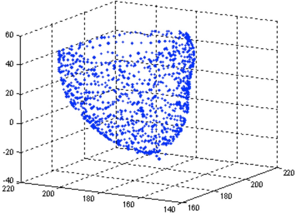
Our experiment is focused on the left ventricle, about 1000 points have been tracked, and about 400 points are distributing on inside-wall while rests are on outside-wall. These points constitute the whole motion of left ventricle in a cardiac cycle, and the points are labeled in several phases, with 0.1 second apart from each other. In the model we focus on the inside-wall surface since the LVV and LVLL is majorly decided by it. <xref ref-type="fig" rid="f1-sensors-10-11428">Figure 1</xref> shows one of the point model.</p></sec>
<sec>
<label>4.2.</label>
<title>LVV and LVL curve interpolation</title>
<p>After the models in all phases are built, the LVV in each moments can be calculated by <xref ref-type="disp-formula" rid="FD1">Equation 1</xref>. These LVV values are <italic>v<sub>i</sub></italic> where <italic>i</italic> = 1,2, ⋯,7. Using the set of <italic>v<sub>i</sub></italic> to interpolate with B-spline method then a LVV curve <italic>C</italic>(<italic>t</italic>) is fitted. The derivative <italic>C</italic>′(<italic>t</italic>) can also be calculated. The curve with solid line in <xref ref-type="fig" rid="f2-sensors-10-11428">Figure 2</xref> is an example of the <italic>C</italic>′(<italic>t</italic>) curve. The landmarks of right Y-axis is corresponding to this curve.</p>
<p>In each inside-wall surface model, finding the centers at top and bottom layer, the LVLL can be calculated by the distance of these two centers. Assuming that the LVLL values are obtained from <italic>m</italic> model, <italic>l<sub>i</sub></italic> where <italic>i</italic> = 1,2, ⋯, <italic>m</italic>, a B-spline curve <italic>L</italic>(<italic>t</italic>) can be fitted with <italic>l<sub>i</sub></italic> and the derivative curve <italic>L</italic>′(<italic>t</italic>) can also be calculated. The curve with dash line in <xref ref-type="fig" rid="f2-sensors-10-11428">Figure 2</xref> is an example of the <italic>L</italic>′(<italic>t</italic>) curve. The landmarks of left Y-axis is corresponding to this curve.</p></sec>
<sec>
<label>4.3.</label>
<title>Measurement of CPP and Tei-index</title>
<p>With the curves of <italic>C</italic>′(<italic>t</italic>) and <italic>L</italic>′(<italic>t</italic>), the partition of CPP can be done by following steps.
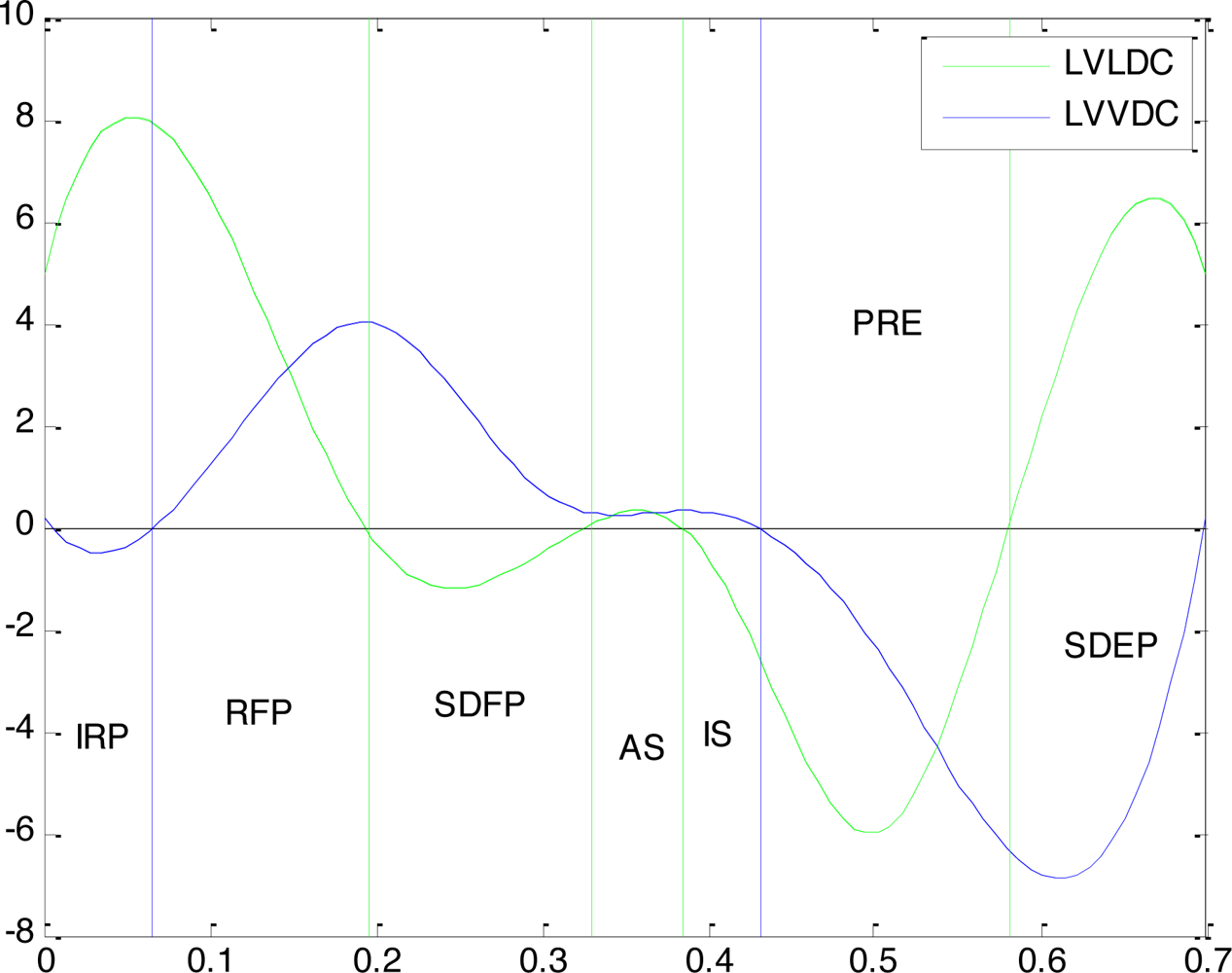
</p>
<list list-type="simple">
<list-item>
<p>Step 1: find the zero-points in <italic>C</italic>′(<italic>t</italic>) as the boundary of systolic and diastolic (blue line in <xref ref-type="fig" rid="f3-sensors-10-11428">Figure 3</xref>);</p></list-item>
<list-item>
<p>Step 2: find the zero-points in <italic>L</italic>′(<italic>t</italic>), to do the further division of CPP(green line in <xref ref-type="fig" rid="f3-sensors-10-11428">Figure 3</xref>).</p></list-item></list>
<p>The final CPP partition result is shown in <xref ref-type="fig" rid="f3-sensors-10-11428">Figure 3</xref>, and the lasting time of each CPP is calculated too. The comparison of the result to the medical statistical average data decided by experts is shown in <xref ref-type="table" rid="t2-sensors-10-11428">Table 2</xref> . Obviously the experiment result is very close to the average data which can prove the validity of this partition.</p>
<p>The Tei index can be calculated by <xref ref-type="disp-formula" rid="FD10">Equation 10</xref>. In this experiment the value of Tei is 0.3617 while the common range of Tei is 0.39±0.05 by medical statistics.</p>
<p>
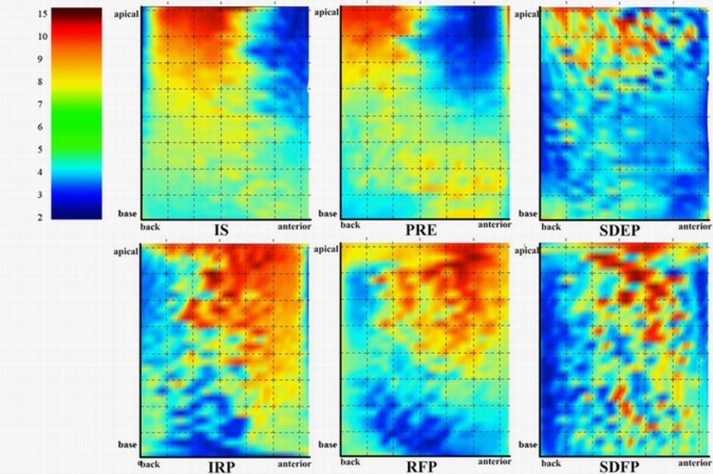
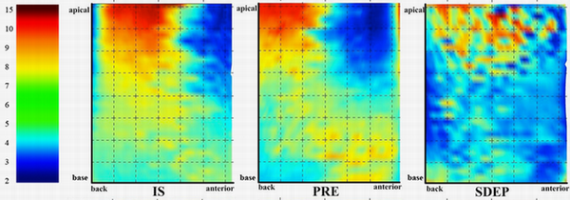
The distribution of LVMA in 6 CPPs is shown in <xref ref-type="fig" rid="f4-sensors-10-11428">Figure 4</xref> (AS is neglected because in that phase the deformation of LV is inconspicuous). It can be seen that the LVMA of LV apical is much larger than that of LV base. During the systole LVMA concentrates in the back of LV while do the opposite during diastolic period. The largest LVMA occurs in IS and IRP which are the beginning of systole and diastole respectively. The result agrees with the medical statistical rule and is very closed to the result of other research [<xref ref-type="bibr" rid="b21-sensors-10-11428">21</xref>,<xref ref-type="bibr" rid="b22-sensors-10-11428">22</xref>].</p></sec></sec>
<sec sec-type="conclusions">
<label>5.</label>
<title>Conclusions</title>
<p>In this paper, a new perspective of myocardial motion analysis, accurate division of cardiac cycle physical phases (CPP), is proposed. Based on this method, an precise and direct calculation of the Tei index is presented. First, several B-spline models of LV inside-wall are built at different time phases. Second, the LVV and LVLL of each model are calculated by B-spline integral and the curves of these two factors are fitted in whole cardiac cycle. Third, the derivative curves of LVV and LVLL are calculated. At last, the CPP partition by finding zero points in them is obtained. The experiment with real human LV data shows the result of this method is very close to the medical statistical values. Tei index is a new heart function index which strongly depends on the CPP. With the accurate CPP division, the accuracy of the direct Tei index calculation method is shown by the experiment result. This paper also proposed a new method to computing LVMA to analyze the myocardial motion. The color figure of LVMA in different CPP shows rules of myocardial motion which are very close to the results of other researches.</p></sec></body>
<back>
<ack>
<p>This work was supported by the National Natural Science Foundation of China and Microsoft Research Asia (60870002, 60802087), NCET, and the Science and Technology Department of Zhejiang Province (2010R10006, 2010C33095, Y1090592).</p></ack>
<ref-list>
<title>References</title>
<ref id="b1-sensors-10-11428"><label>1.</label><citation citation-type="journal"><person-group person-group-type="author"><name><surname>Shling</surname><given-names>M</given-names></name><name><surname>Arigovindan</surname><given-names>M</given-names></name><name><surname>Jansen</surname><given-names>C</given-names></name><name><surname>Hunziker</surname><given-names>P</given-names></name><name><surname>Unser</surname><given-names>M</given-names></name></person-group><article-title>Myocardial Motion Analysis From B-Mode Echocardiograms</article-title><source>IEEE Trans Image Process</source><year>2005</year><volume>14</volume><fpage>525</fpage><lpage>536</lpage><pub-id pub-id-type="doi">10.1109/TIP.2004.838709</pub-id><pub-id pub-id-type="pmid">15825486</pub-id></citation></ref>
<ref id="b2-sensors-10-11428"><label>2.</label><citation citation-type="confproc"><person-group person-group-type="author"><name><surname>Wang</surname><given-names>X</given-names></name><name><surname>Metaxas</surname><given-names>D</given-names></name><name><surname>Chen</surname><given-names>T</given-names></name><name><surname>Axel</surname><given-names>L</given-names></name></person-group><article-title>Meshless deformable models for LV motion analysis</article-title><conf-name>Proceedings of IEEE Conference on Computer Vision and Pattern Recognition</conf-name><conf-loc>Anchorage, AK, USA</conf-loc><conf-date>June 2008</conf-date><fpage>1</fpage><lpage>8</lpage></citation></ref>
<ref id="b3-sensors-10-11428"><label>3.</label><citation citation-type="journal"><person-group person-group-type="author"><name><surname>Sundar</surname><given-names>H</given-names></name><name><surname>Litt</surname><given-names>H</given-names></name><name><surname>Shen</surname><given-names>D</given-names></name></person-group><article-title>Estimating myocardial motion by 4D image warping</article-title><source>Pattern Recognit</source><year>2009</year><volume>42</volume><fpage>2514</fpage><lpage>2526</lpage><pub-id pub-id-type="doi">10.1016/j.patcog.2009.04.022</pub-id><pub-id pub-id-type="pmid">20379351</pub-id></citation></ref>
<ref id="b4-sensors-10-11428"><label>4.</label><citation citation-type="journal"><person-group person-group-type="author"><name><surname>Tei</surname><given-names>C</given-names></name></person-group><article-title>New Noninvasive Index for Combined Systolic and Diastolic Ventricular Function</article-title><source>J Cardiol</source><year>1995</year><volume>26</volume><fpage>135</fpage><lpage>136</lpage><pub-id pub-id-type="pmid">7674144</pub-id></citation></ref>
<ref id="b5-sensors-10-11428"><label>5.</label><citation citation-type="journal"><person-group person-group-type="author"><name><surname>Pellett</surname><given-names>AA</given-names></name><name><surname>Tolar</surname><given-names>WG</given-names></name><name><surname>Merwin</surname><given-names>DG</given-names></name><name><surname>Kerut</surname><given-names>EK</given-names></name></person-group><article-title>The Tei Index: Methodology and Disease State Values</article-title><source>Echocardiography</source><year>2004</year><volume>21</volume><fpage>669</fpage><lpage>672</lpage><pub-id pub-id-type="doi">10.1111/j.0742-2822.2004.04052.x</pub-id><pub-id pub-id-type="pmid">15488100</pub-id></citation></ref>
<ref id="b6-sensors-10-11428"><label>6.</label><citation citation-type="journal"><person-group person-group-type="author"><name><surname>Sutton</surname><given-names>MSJ</given-names></name><name><surname>Wiegers</surname><given-names>SE</given-names></name></person-group><article-title>The Tei index—a role in the diagnosis of heart failure</article-title><source>Eur Heart J</source><year>2000</year><volume>21</volume><fpage>1888</fpage><lpage>1895</lpage><pub-id pub-id-type="doi">10.1053/euhj.2000.2246</pub-id><pub-id pub-id-type="pmid">11052862</pub-id></citation></ref>
<ref id="b7-sensors-10-11428"><label>7.</label><citation citation-type="journal"><person-group person-group-type="author"><name><surname>Lakoumentas</surname><given-names>JA</given-names></name><name><surname>Panou</surname><given-names>FK</given-names></name><name><surname>Kotseroglou</surname><given-names>VK</given-names></name><name><surname>Aggeli</surname><given-names>KI</given-names></name><name><surname>Harbis</surname><given-names>PK</given-names></name></person-group><article-title>The Tei Index of Myocardial Performance: Applications in Cardiology</article-title><source>Hellenic J Cardiol</source><year>2005</year><volume>46</volume><fpage>52</fpage><lpage>58</lpage><pub-id pub-id-type="pmid">15807396</pub-id></citation></ref>
<ref id="b8-sensors-10-11428"><label>8.</label><citation citation-type="journal"><person-group person-group-type="author"><name><surname>Masugata</surname><given-names>H</given-names></name><name><surname>Senda</surname><given-names>S</given-names></name><name><surname>Goda</surname><given-names>F</given-names></name><name><surname>Yamagami</surname><given-names>A</given-names></name><name><surname>Okuyama</surname><given-names>H</given-names></name><name><surname>Kohno</surname><given-names>T</given-names></name><name><surname>Hosomi</surname><given-names>N</given-names></name><name><surname>Yukiiri</surname><given-names>K</given-names></name><name><surname>Noma</surname><given-names>T</given-names></name><name><surname>Murao</surname><given-names>K</given-names></name><name><surname>Nishiyama</surname><given-names>A</given-names></name><name><surname>Kohno</surname><given-names>M</given-names></name></person-group><article-title>Independent Determinants of the Tei Index in Hypertensive Patients With Preserved Left Ventricular Systolic Function</article-title><source>Int Heart J</source><year>2009</year><volume>50</volume><fpage>331</fpage><lpage>340</lpage><pub-id pub-id-type="doi">10.1536/ihj.50.331</pub-id><pub-id pub-id-type="pmid">19506337</pub-id></citation></ref>
<ref id="b9-sensors-10-11428"><label>9.</label><citation citation-type="journal"><person-group person-group-type="author"><name><surname>Comas</surname><given-names>M</given-names></name><name><surname>Crispi</surname><given-names>F</given-names></name><name><surname>Cruz-Martinez</surname><given-names>R</given-names></name><name><surname>Martinez</surname><given-names>JM</given-names></name><name><surname>Figueras</surname><given-names>F</given-names></name><name><surname>Gratacs</surname><given-names>E</given-names></name></person-group><article-title>Usefulness of myocardial tissue Doppler vs conventional echocardiography in the evaluation of cardiac dysfunction in early-onset intrauterine growth restriction</article-title><source>Am J Obstet Gynecol</source><year>2010</year><volume>203</volume><fpage>45.e1</fpage><lpage>45.e7</lpage><pub-id pub-id-type="doi">10.1016/j.ajog.2010.02.044</pub-id></citation></ref>
<ref id="b10-sensors-10-11428"><label>10.</label><citation citation-type="confproc"><person-group person-group-type="author"><name><surname>Guan</surname><given-names>Q</given-names></name><name><surname>Du</surname><given-names>Y</given-names></name><name><surname>Chen</surname><given-names>SY</given-names></name><name><surname>Wang</surname><given-names>F</given-names></name></person-group><article-title>Calculation of Tei Index and LV Motion Amplitude Based on Cardiac Physical Phase</article-title><conf-name>Proceedings of IEEE International Conference on Robotics and Biomimetics</conf-name><conf-loc>Guilin, China</conf-loc><conf-date>December 2009</conf-date><fpage>1027</fpage><lpage>1031</lpage></citation></ref>
<ref id="b11-sensors-10-11428"><label>11.</label><citation citation-type="other"><person-group person-group-type="author"><name><surname>Greenberg</surname><given-names>NL</given-names></name><name><surname>Popovic</surname><given-names>ZB</given-names></name><name><surname>Saracino</surname><given-names>G</given-names></name><name><surname>Grimm</surname><given-names>RA</given-names></name><name><surname>Thomas</surname><given-names>JD</given-names></name></person-group><article-title>Novel time-varying 3D display of wall motion, strain, strain rate and torsion for LV function assessment</article-title><conf-name>Proceedings of Computers in Cardiology</conf-name><conf-loc>Bologna, Italy</conf-loc><conf-date>September 2008</conf-date><fpage>21</fpage><lpage>23</lpage></citation></ref>
<ref id="b12-sensors-10-11428"><label>12.</label><citation citation-type="journal"><person-group person-group-type="author"><name><surname>Nichols</surname><given-names>KJ</given-names></name><name><surname>van Tosh</surname><given-names>A</given-names></name><name><surname>Wang</surname><given-names>Y</given-names></name><name><surname>Reichek</surname><given-names>N</given-names></name><name><surname>Palestro</surname><given-names>CJ</given-names></name></person-group><article-title>Automated versus manual detection of left ventricular wall motion abnormalities by gated blood pool SPECT</article-title><source>Med Phys</source><year>2009</year><volume>36</volume><fpage>1251</fpage><lpage>1257</lpage><pub-id pub-id-type="doi">10.1118/1.3095774</pub-id><pub-id pub-id-type="pmid">19472633</pub-id></citation></ref>
<ref id="b13-sensors-10-11428"><label>13.</label><citation citation-type="journal"><person-group person-group-type="author"><name><surname>Mark</surname><given-names>M</given-names></name><name><surname>Schneider</surname><given-names>B</given-names></name><name><surname>Hennig</surname><given-names>J</given-names></name></person-group><article-title>Fast phase contrast cardiac magnetic resonance imaging: Improved assessment and analysis of left ventricular wall motion</article-title><source>J Magn Reson Imaging</source><year>2002</year><volume>15</volume><fpage>642</fpage><lpage>653</lpage><pub-id pub-id-type="doi">10.1002/jmri.10114</pub-id><pub-id pub-id-type="pmid">12112514</pub-id></citation></ref>
<ref id="b14-sensors-10-11428"><label>14.</label><citation citation-type="journal"><person-group person-group-type="author"><name><surname>Oki</surname><given-names>T</given-names></name><name><surname>Iuchi</surname><given-names>A</given-names></name><name><surname>Tabata</surname><given-names>T</given-names></name><name><surname>Mishiro</surname><given-names>Y</given-names></name><name><surname>Yamada</surname><given-names>H</given-names></name><name><surname>Abe</surname><given-names>M</given-names></name><name><surname>Onose</surname><given-names>Y</given-names></name><name><surname>Wakatsuki</surname><given-names>T</given-names></name><name><surname>Ito</surname><given-names>S</given-names></name></person-group><article-title>Left Ventricular Systolic Wall Motion Velocities Along the Long and Short Axes Measured by Pulsed Tissue Doppler Imaging in Patients with Atrial Fibrillation</article-title><source>J Am Soc Echocardiogr</source><year>1999</year><volume>12</volume><fpage>121</fpage><lpage>128</lpage><pub-id pub-id-type="doi">10.1016/S0894-7317(99)70124-0</pub-id><pub-id pub-id-type="pmid">9950971</pub-id></citation></ref>
<ref id="b15-sensors-10-11428"><label>15.</label><citation citation-type="journal"><person-group person-group-type="author"><name><surname>Azhari</surname><given-names>H</given-names></name><name><surname>Sideman</surname><given-names>S</given-names></name><name><surname>Weiss</surname><given-names>JL</given-names></name><name><surname>Shapiro</surname><given-names>EP</given-names></name><name><surname>Weisfeldt</surname><given-names>ML</given-names></name><name><surname>Graves</surname><given-names>WL</given-names></name><name><surname>Rogers</surname><given-names>WJ</given-names></name><name><surname>Beyar</surname><given-names>R</given-names></name></person-group><article-title>Three-dimensional Mapping of Acute Ischemic Regions Using MRI: Wall Thickening Versus Motion Analysis</article-title><source>Am J Physiol</source><year>1990</year><volume>259</volume><fpage>H1492</fpage><lpage>H1503</lpage><pub-id pub-id-type="pmid">2240248</pub-id></citation></ref>
<ref id="b16-sensors-10-11428"><label>16.</label><citation citation-type="confproc"><person-group person-group-type="author"><name><surname>Qin</surname><given-names>K</given-names></name></person-group><article-title>General Matrix Representations for B-Splines and Applications</article-title><conf-name>Proceedings of the Sixth Pacific Conference on Computer Graphics and Applications</conf-name><conf-loc>Singapore</conf-loc><conf-date>October 1998</conf-date><fpage>37</fpage><lpage>43</lpage></citation></ref>
<ref id="b17-sensors-10-11428"><label>17.</label><citation citation-type="journal"><person-group person-group-type="author"><name><surname>Wang</surname><given-names>X</given-names></name><name><surname>Sun</surname><given-names>J</given-names></name><name><surname>Qin</surname><given-names>K</given-names></name></person-group><article-title>Symbolic Matrix Representation of NURBS and Its Application</article-title><source>Chin J Comput</source><year>1993</year><volume>16</volume><fpage>29</fpage><lpage>34</lpage></citation></ref>
<ref id="b18-sensors-10-11428"><label>18.</label><citation citation-type="confproc"><person-group person-group-type="author"><name><surname>Jiang</surname><given-names>TT</given-names></name><name><surname>Chen</surname><given-names>SY</given-names></name></person-group><article-title>3-D representation and volumetric measurement of human heart from a cylindrical B-Spline surface model</article-title><conf-name>Proceedings of The International Conference on BioMedical Engineering and Informatics</conf-name><conf-loc>Sanya, China</conf-loc><conf-date>May 2008</conf-date><fpage>765</fpage><lpage>769</lpage></citation></ref>
<ref id="b19-sensors-10-11428"><label>19.</label><citation citation-type="journal"><person-group person-group-type="author"><name><surname>Mirsky</surname><given-names>I</given-names></name></person-group><article-title>Assessment of passive elastic stiffiness of cardiac muscle: Mathematical concepts, physiologic and clinical considerations, directions of future research</article-title><source>Prog Cardiologic Dis</source><year>1976</year><volume>17</volume><fpage>277</fpage><lpage>281</lpage></citation></ref>
<ref id="b20-sensors-10-11428"><label>20.</label><citation citation-type="journal"><person-group person-group-type="author"><name><surname>Cootes</surname><given-names>TF</given-names></name><name><surname>Taylor</surname><given-names>CJ</given-names></name><name><surname>Cooper</surname><given-names>DH</given-names></name><name><surname>Graham</surname><given-names>J</given-names></name></person-group><article-title>Active shape models — their training and application</article-title><source>Comput Vis Image Understand</source><year>1995</year><volume>61</volume><fpage>38</fpage><lpage>59</lpage><pub-id pub-id-type="doi">10.1006/cviu.1995.1004</pub-id></citation></ref>
<ref id="b21-sensors-10-11428"><label>21.</label><citation citation-type="journal"><person-group person-group-type="author"><name><surname>Jinah</surname><given-names>P</given-names></name><name><surname>Metaxas</surname><given-names>D</given-names></name><name><surname>Young</surname><given-names>AA</given-names></name><name><surname>Axel</surname><given-names>L</given-names></name></person-group><article-title>Deformation models with parameter functions for cardiac motion analysis from tagged MRI data</article-title><source>IEEE Med Image</source><year>1996</year><volume>15</volume><fpage>278</fpage><lpage>289</lpage><pub-id pub-id-type="doi">10.1109/42.500137</pub-id></citation></ref>
<ref id="b22-sensors-10-11428"><label>22.</label><citation citation-type="journal"><person-group person-group-type="author"><name><surname>Maroko</surname><given-names>PR</given-names></name></person-group><article-title>Modification of myocardial infarction size after coronary occlusion</article-title><source>Ann Int Med</source><year>1973</year><volume>79</volume><fpage>720</fpage><lpage>733</lpage><pub-id pub-id-type="pmid">4148053</pub-id></citation></ref></ref-list>
<sec sec-type="display-objects">
<title>Figures and Tables</title>
<fig id="f1-sensors-10-11428" position="float">
<label>Figure 1.</label>
<caption>
<p>An example of the LV endocardium point model at one time phase.</p></caption>
<graphic xlink:href="sensors-10-11428f1.gif"/></fig>
<fig id="f2-sensors-10-11428" position="float">
<label>Figure 2.</label>
<caption>
<p>LVV varying cure (solid line) and LVLL varying cure (dash line) in whole cardiac cycle.</p></caption>
<graphic xlink:href="sensors-10-11428f2.gif"/></fig>
<fig id="f3-sensors-10-11428" position="float">
<label>Figure 3.</label>
<caption>
<p>CPP partition in cardiac cycle.</p></caption>
<graphic xlink:href="sensors-10-11428f3.gif"/></fig>
<fig id="f4-sensors-10-11428" position="float">
<label>Figure 4.</label>
<caption>
<p>LVMA color graph of 6 CPPs. The color band in left column indicates the value of LVMA.</p></caption>
<graphic xlink:href="sensors-10-11428f4.gif"/></fig>
<table-wrap id="t1-sensors-10-11428" position="float">
<label>Table 1.</label>
<caption>
<p>LVV and LVLL Features of Each CPP.</p></caption>
<table frame="box" rules="all">
<thead>
<tr>
<th align="left" valign="top"/>
<th align="center" valign="top"><italic>CPP</italic></th>
<th align="center" valign="top"><italic>LVV</italic> (<italic>C</italic>(<italic>t</italic>))</th>
<th align="center" valign="top"><italic>C′</italic>(<italic>t</italic>)</th>
<th align="center" valign="top"><italic>LV LL</italic>(<italic>L</italic>(<italic>t</italic>))</th>
<th align="center" valign="top"><italic>L′</italic>(<italic>t</italic>)</th></tr></thead>
<tbody>
<tr>
<td align="center" valign="middle" rowspan="3">Systolic</td>
<td align="center" valign="middle">IS</td>
<td align="center" valign="middle">Hold on</td>
<td align="center" valign="middle"><italic>≈</italic> 0</td>
<td align="center" valign="middle">Reduce</td>
<td align="center" valign="middle"><italic>&lt;</italic> 0</td></tr>
<tr>
<td align="center" valign="middle">REP</td>
<td align="center" valign="middle">Reduce</td>
<td align="center" valign="middle"><italic>&lt;</italic> 0</td>
<td align="center" valign="middle">Reduce</td>
<td align="center" valign="middle"><italic>&lt;</italic> 0</td></tr>
<tr>
<td align="center" valign="middle">SDEP</td>
<td align="center" valign="middle">Reduce</td>
<td align="center" valign="middle"><italic>&lt;</italic> 0</td>
<td align="center" valign="middle">Increase</td>
<td align="center" valign="middle"><italic>&gt;</italic> 0</td></tr>
<tr>
<td align="center" valign="middle" rowspan="3">Diastolic</td>
<td align="center" valign="middle">IRP</td>
<td align="center" valign="middle">Hold on</td>
<td align="center" valign="middle"><italic>≈</italic> 0</td>
<td align="center" valign="middle">Increase</td>
<td align="center" valign="middle"><italic>&gt;</italic> 0</td></tr>
<tr>
<td align="center" valign="middle">RFP</td>
<td align="center" valign="middle">Increase</td>
<td align="center" valign="middle"><italic>&gt;</italic> 0</td>
<td align="center" valign="middle">Increase</td>
<td align="center" valign="middle"><italic>&gt;</italic> 0</td></tr>
<tr>
<td align="center" valign="middle">SDFP</td>
<td align="center" valign="middle">Increase</td>
<td align="center" valign="middle"><italic>&gt;</italic> 0</td>
<td align="center" valign="middle">Reduce</td>
<td align="center" valign="middle"><italic>&lt;</italic> 0</td></tr>
<tr>
<td align="center" valign="middle"/>
<td align="center" valign="middle">AS</td>
<td align="center" valign="middle">Hold on</td>
<td align="center" valign="middle"><italic>≈</italic> 0</td>
<td align="center" valign="middle">Hold on</td>
<td align="center" valign="middle"><italic>≈</italic> 0</td></tr></tbody></table></table-wrap>
<table-wrap id="t2-sensors-10-11428" position="float">
<label>Table 2.</label>
<caption>
<p>CPP Lasting Time.</p></caption>
<table frame="box" rules="all">
<thead>
<tr>
<th align="center" valign="top">Phase</th>
<th align="center" valign="top">Average data</th>
<th align="center" valign="top">Result</th></tr></thead>
<tbody>
<tr>
<td align="center" valign="top">IS</td>
<td align="center" valign="top">0.06–0.08</td>
<td align="center" valign="top">0.066</td></tr>
<tr>
<td align="center" valign="top">PRE</td>
<td align="center" valign="top">0.11</td>
<td align="center" valign="top">0.128</td></tr>
<tr>
<td align="center" valign="top">SDEP</td>
<td align="center" valign="top">0.14</td>
<td align="center" valign="top">0.132</td></tr>
<tr>
<td align="center" valign="top">IRP</td>
<td align="center" valign="top">0.06–0.08</td>
<td align="center" valign="top">0.057</td></tr>
<tr>
<td align="center" valign="top">RFP</td>
<td align="center" valign="top">0.11</td>
<td align="center" valign="top">0.047</td></tr>
<tr>
<td align="center" valign="top">SDFP</td>
<td align="center" valign="top">0.12</td>
<td align="center" valign="top">0.151</td></tr>
<tr>
<td align="center" valign="top">AS</td>
<td align="center" valign="top">0.1</td>
<td align="center" valign="top">0.119</td></tr></tbody></table></table-wrap></sec></back></article>
