Analysis of Large Scale Spatial Variability of Soil Moisture Using a Geostatistical Method

Abstract
:
1. Introduction
2. Study Area and Data Sets
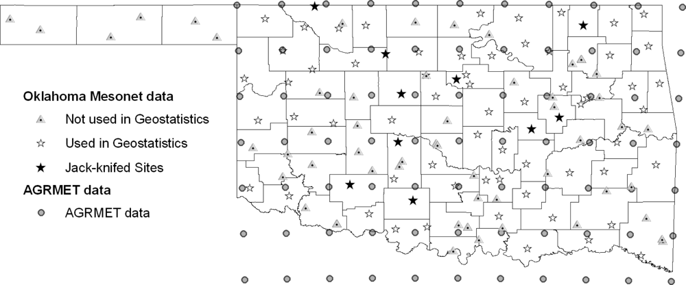
2.1. In Situ Oklahoma Mesonet
2.2. AGRMET Model
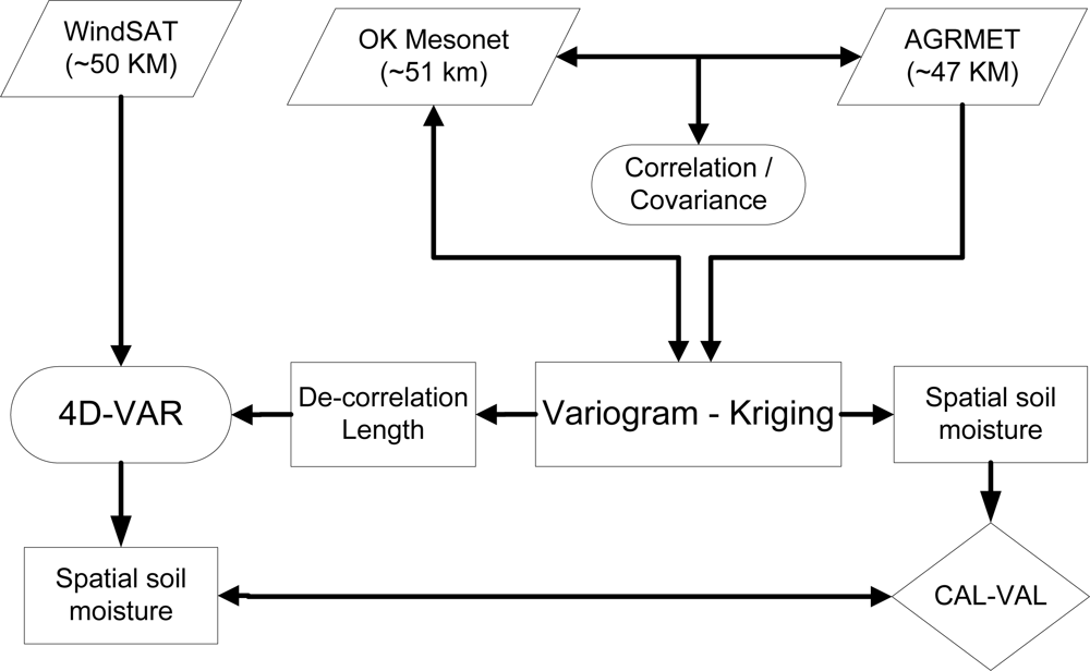
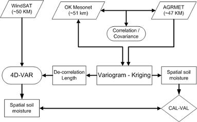
3. Methodology
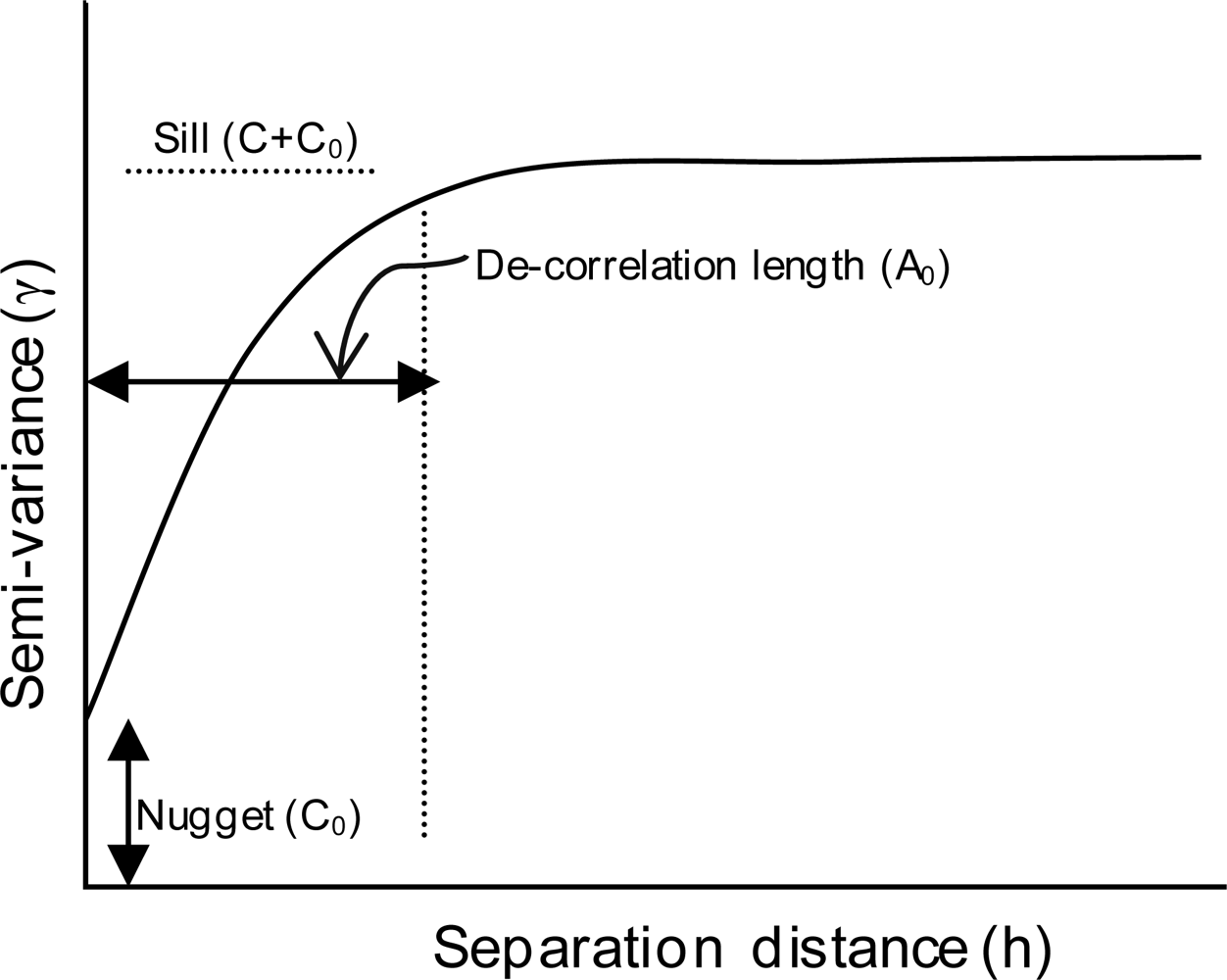
3.1. Variogram and Kriging
- γ(h) = semivariance for interval distance class h;
- h = the separation distance interval
- C0 = nugget variance ≥ 0;
- C = structural variance ≥ C0; and
- A0 = decorrelation length or range parameter.
3.2. Geostatistical Spatial Analysis
3.3. Oklahoma Mesonet Data Screening and Quality Control
4. Results and Discussion
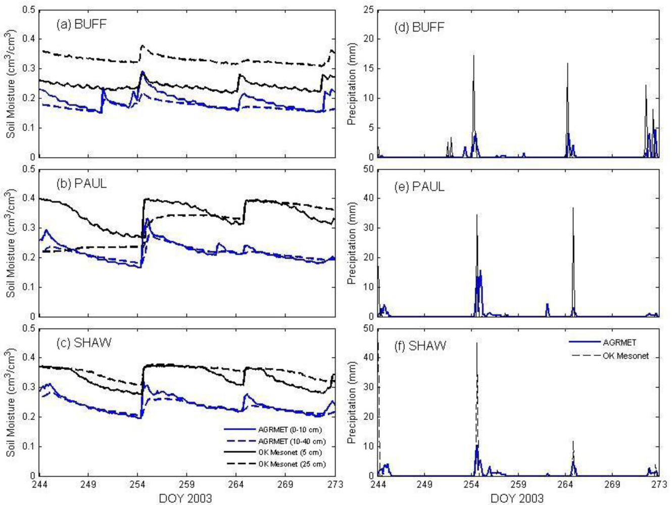
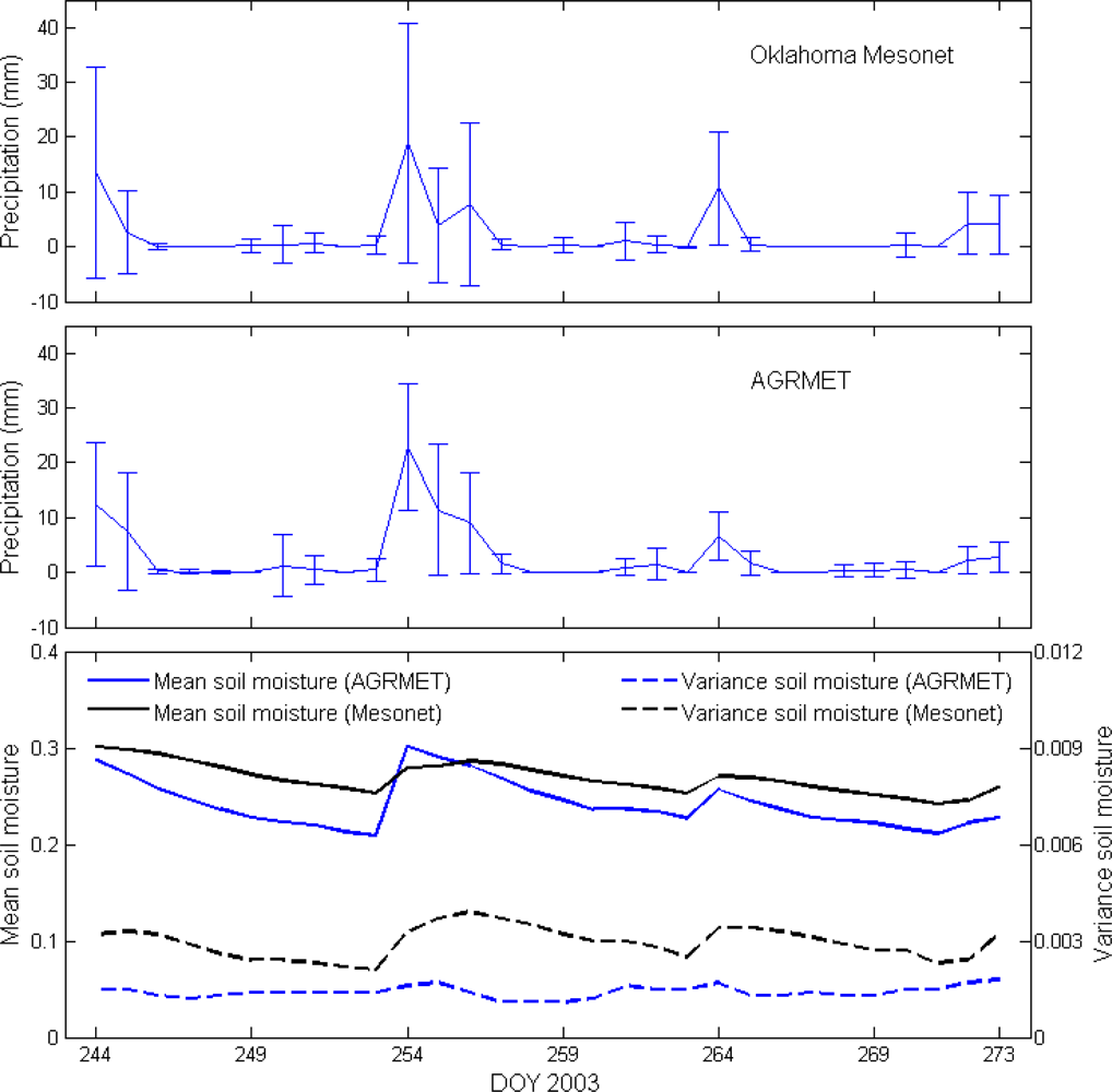
4.1. In Situ and Model Soil Moisture Comparison (Oklahoma Mesonet vs. AGRMET)
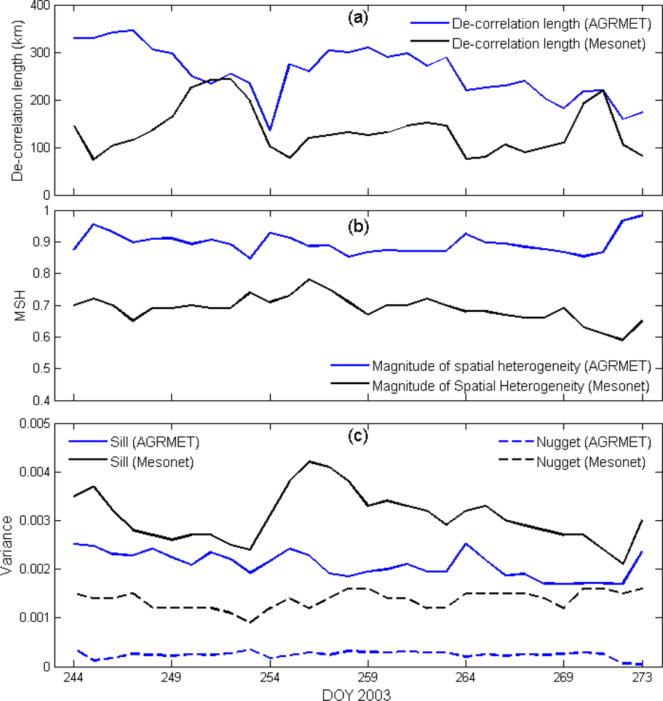
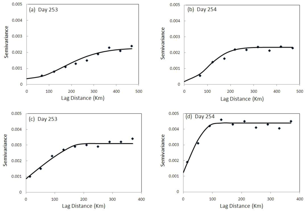
4.2. Variogram Analysis of Soil Moisture
4.3. Kriging Performance Assessment
5. Summary and Conclusions
Acknowledgments
References and Notes
- Entekhabi, D.; Asrar, G.R.; Betts, A.K.; Beven, K.J.; Bras, R.L.; Duffy, C.J.; Dunne, T.; Koster, R.D.; Lettenmaier, D.P.; McLaughlin, D.B.; Shuttleworth, W.J.; van Genuchten, M.T.; Wei, M.Y.; Wood, E.F. An Agenda for Land Surface Hydrology Research and a Call for the Second International Hydrological Decade. B. Am. Meteorol. Soc 1999, 80, 2043–2058. [Google Scholar]
- De Lannoy, G.J.M.; Verhoest, N.E.C.; Houser, P.R.; Gish, T.J.; Meirvenne, V.M. Spatial and Temporal Characteristics of Soil Moisture in an Intensively Monitored Agricultural Field (OPE3). J. Hydrol 2006, 331, 719–730. [Google Scholar]
- Reichle, R.H.; Koster, R.D.; Liu, P.; Mahanama, S.P.; Njoku, E.G.; Owe, M. Comparison and Assimilation of Global Soil Moisture Retrievals from the Advanced Microwave Scanning Radiometer for the Earth Observing System (AMSR-E) and the Scanning Multichannel Microwave Radiometer (SMMR). J. Geophys. Res 2007, 112, D09108. [Google Scholar]
- Jones, A.S.; Vukicevic, T.; Vonder-Haar, T.H. A Microwave Satellite Observational Operator for Variational Data Assimilation of Soil Moisture. J. Hydrometeorol 2004, 5, 213–229. [Google Scholar]
- Durand, M.; Margulis, S.A. Effects of Uncertainty Magnitude and Accuracy on Assimilation of Multiscale Measurements for Snowpack Characterization. J. Geophys. Res 2008, 113, D02105. [Google Scholar]
- Bolten, J.D.; Crow, W.T.; Zhan, X.; Reynolds, C.A.; Jackson, T.J. Assimilation of a Satellite-Based SoilMoisture Product into a Two-Layer Water Balance Model for a Global Crop Production Decision Support System; Springer: Berlin, Germany, 2009; pp. 449–463. [Google Scholar]
- Oldak, A.; Jackson, T.; Pachepsky, Y. Using GIS in Passive Microwave Soil Mapping and Geostatistical Analysis. Int. J. Geogr. Inf. Sci 2002, 16, 681–689. [Google Scholar]
- Teuling, A.J.; Troch, P.A. Improved Understanding of Soil Moisture Variability Dynamics. Geophys. Res. Lett 2005, 32, L05404. [Google Scholar]
- Zupanski, M.; Zupanski, D.; Parrish, D.F.; Rogers, E.; DiMego, G. Four-Dimensional Variational Data Assimilation for the Blizzard of 2000. Mon. Weather. Rev 2002, 130, 1967–1988. [Google Scholar]
- Vukicevic, T.; Sengupta, M.; Jones, A.S.; Vonder-Haar, T. Cloud-Resolving Satellite Data Assimilation: Information Content of IR Window Observations and Uncertainties in Estimation. J. Atmos. Sci. (JAS) 2006, 63, 901–919. [Google Scholar]
- Crow, W.T. Correcting Land Surface Model Predictions for the Impact of Temporally Sparse Rainfall Rate Measurements Using an Ensemble Kalman Filter and Surface Brightness Temperature Observations. J. Hydrometeorol 2003, 4, 960–973. [Google Scholar]
- Zupanski, M.; Fletcher, S.J.; Navon, I.M.; Uzunoglu, B.; Heikes, R.P.; Randall, D.A.; Ringler, T.D.; Daescu, D.N. Initiation of Ensemble Data Assimilation. Tellus A 2006, 58, 159–170. [Google Scholar]
- Wang, J.; Fu, B.; Qiu, Y.; Chen, L.; Wang, Z. Geostatistical Analysis of Soil Moisture Variability on Da Nangou Catchment of the Loess Plateau, China. Environ. Geol 2001, 41, 113–120. [Google Scholar]
- Western, A.W.; Grayson, R.B.; Green, T.R. The Tarrawarra Project: High Resolution Spatial Measurement, Modelling and Analysis of Hydrological Response. Hydrol. Process 1999, 13, 633–652. [Google Scholar]
- Western, A.W.; Bloschl, G. On the Spatial Scaling of Soil Moisture. J. Hydrol 1999, 217, 203–224. [Google Scholar]
- Bardossy, A.; Lehmann, W. Spatial Distribution of Soil Moisture in a Small Catchment. Part 1: geostatistical analysis. J. Hydrol 1998, 206, 1–15. [Google Scholar]
- Herbst, M.; Diekkruger, B. Modelling the Spatial Variability of Soil Moisture in a Micro-Scale Catchment and Comparison with Field Data Using Geostatistics. Phys. Chem. Earth. Pt A/B/C 2003, 28, 239–245. [Google Scholar]
- Anctil, F.; Mathieu, R.; Parent, L.E.; Viau, A.A.; Sbih, M.; Hessami, M. Geostatistics of Near-Surface Moisture in Bare Cultivated Organic Soils. J. Hydrol 2002, 260, 30–37. [Google Scholar]
- Hoff, C. Spatial and Temporal Persistence of Mean Monthly Temperature on Two GCM Grid Cells. Int. J. Climat 2001, 21, 731–744. [Google Scholar]
- Rodell, M.; Houser, R.P.; Jambor, U.; Gottschalck, J.; Mitchell, K.; Meng, J.C.; Arsenault, K.; Cosgrove, B.; Radakovich, J.; Bosilovich, M.; Entin, K.J.; Walker, P.J.; Lohmann, D.; Toll, D. The Global Land Data Assimilation System. B. Am. Meteorol. Soc 2004, 85, 381–394. [Google Scholar]
- McPherson, R.A.; Fiebrich, C.A.; Crawford, K.C.; Elliott, R.L.; Kilby, J.R.; Grimsley, D.L.; Martinez, J.E.; Basara, J.B.; Illston, B.G.; Morris, D.A.; Kloesel, K.A.; Stadler, S.J.; Melvin, A.D.; Sutherland, A.J.; Shrivastava, H.; Carlson, J.D.; Wolfinbarger, J.M.; Bostic, J.P.; Demko, D.B. Statewide Monitoring of the Mesoscale Environment: A Technical Update on the Oklahoma Mesonet. J. Atmos. Oceanic Technol 2007, 24, 301–321. [Google Scholar]
- Brock, F.V.; Crawford, K.C.; Elliot, R.L.; Cuperus, G.W.; Stadler, S.J.; Johnson, H.L.; Eilts, M.D. The Oklahoma Mesonet: A Technical Overview. J. Atmos. Oceanic Technol 1995, 12, 5–19. [Google Scholar]
- Illston, B.G.; Basara, J.B.; Fisher, D.K.; Elliott, R.; Fiebrich, C.A.; Crawford, K.C.; Humes, K.; Hunt, E. Mesoscale Monitoring of Soil Moisture Across a Statewide Network. J. Atmos. Oceanic Technol 2008, 25, 167–182. [Google Scholar]
- Gayno, G.; Wegiel, J. Incorporating Global Real-Time Surface Fields into MM5 at the Air Force Weather Agency; 10th Penn State/NCAR MM5 Users’ Workshop: Boulder, CO, USA, 2000; pp. 62–65. [Google Scholar]
- AWFA. Data format handbook for AGRMET. 2002. Available online: http://www.mmm.ucar.edu/mm5/documents/DATA_FORMAT_HANDBOOK.pdf (accessed on January 20, 2010).
- Webster, R.; Oliver, M.A. Geostatistics for Environmental Scientists; John Wiley & Sons Ltd: Hoboken, NJ, USA, 2001. [Google Scholar]
- Matheron, G. La théorie des variables régionalisé es et ses applications; Masson et Cie: Paris, France, 1965. [Google Scholar]
- Isaaks, E.H.; Srivastava, R.M. Applied geostatistics; Oxford University Press: New York, NY, USA, 1989. [Google Scholar]
- Rossi, R.E.; Dungan, J.L.; Beck, L.R. Kriging in the Shadows: Geostatistical Interpolation for Remote Sensing. Remote Sens. Environ 1994, 49, 32–40. [Google Scholar]
- Bhatti, A.U.; Mulla, D.J.; Frazier, B.E. Estimation of Soil Properties and Wheat Yields on Complex Eroded Hills Using Geostatistics and Thematic Mapper Images. Remote Sens. Environ 1991, 37, 181–191. [Google Scholar]
- Genton, M. Variogram Fitting by Generalized Least Squares Using an Explicit Formula for the Covariance Structure. Math. Geol 1998, 30, 323–345. [Google Scholar]
- Bishop, T.F.A.; McBratney, A.B. A Comparison of Prediction Methods for the Creation of Field-Extent Soil Property Maps. Geoderma 2001, 103, 149–160. [Google Scholar]
- Reynolds, S.G. The Gravimetric Method of Soil Moisture Determination, part III, An Examination of Factors inFluencing Soil Moisture Variability. J. Hydrol 1970, 11, 288–300. [Google Scholar]
- Hollingsworth, A.; Lönnberg, P. The Statistical Structure of Short-Range Forecast Errors as Determined from Radiosonde data. Part I: The Wind Field. Tellus 1986, 38A, 111–136. [Google Scholar]
- Haberlandt, U. Geostatistical Interpolation of Hourly Precipitation from Rain Gauges and Radar for a Large-Scale Extreme Rainfall Event. J. Hydrol 2007, 332, 144–157. [Google Scholar]
- Boerner, R.E.J.; Scherzer, A.J.; Brinkman, J.A. Spatial Patterns of Inorganic N, P Availability, and Organic C in Relation to Soil Disturbance: A Chronosequence Analysis. Appl. Soil. Ecol 1998, 7, 159–177. [Google Scholar]
- Merlin, O.; Chehbouni, A.; Kerr, Y.H.; Goodrich, D.C. A Downscaling Method for Distributing Surface Soil Moisture Within a Microwave Pixel: Application to the Monsoon ‘90 Data. Remote Sens. Environ 2006, 101, 379–389. [Google Scholar]
- Jones, A.S.; Combs, C.L.; Longmore, S.; Lakhankar, T.; Mason, G.; McWilliams, G.; Mungiole, M.; Rapp, D.; Vonder-Haar, T.H.; Vukicevic, T. NPOESS Soil Moisture Satellite Data Assimilation Research Using WindSat data. Proceedings of Third Symposium on Future National Operational Environmental Satellite Systems—Strengthening Our Understanding of Weather and Climate, January 16–17; San Antonio, TX, USA, 2007. [Google Scholar]


| Site Name | Latitude | Longitude | Bias | RMSE | Correlation Coefficient |
|---|---|---|---|---|---|
| KETC | 34.529 | −97.765 | −0.059 | 0.060 | 0.81 |
| KING | 35.881 | −97.911 | +0.027 | 0.030 | 0.97 |
| LAHO | 36.384 | −98.111 | −0.006 | 0.008 | 0.94 |
| MARE | 36.064 | −97.213 | +0.047 | 0.048 | 0.86 |
| MAYR | 36.987 | −99.011 | +0.012 | 0.013 | 0.80 |
| MEDI | 34.729 | −98.567 | +0.060 | 0.061 | 0.94 |
| MINC | 35.272 | −97.956 | −0.023 | 0.026 | 0.86 |
| NOWA | 36.744 | −95.608 | −0.027 | 0.032 | 0.46 |
| OKEM | 35.432 | −96.263 | −0.025 | 0.026 | 0.86 |
| OKMU | 35.581 | −95.915 | −0.011 | 0.013 | 0.91 |
| All Sites | -- | -- | -- | 0.032 | 0.84 |
©2010 by the authors; licensee Molecular Diversity Preservation International, Basel, Switzerland. This article is an open access article distributed under the terms and conditions of the Creative Commons Attribution license (http://creativecommons.org/licenses/by/3.0/)
Share and Cite
Lakhankar, T.; Jones, A.S.; Combs, C.L.; Sengupta, M.; Vonder Haar, T.H.; Khanbilvardi, R. Analysis of Large Scale Spatial Variability of Soil Moisture Using a Geostatistical Method. Sensors 2010, 10, 913-932. https://doi.org/10.3390/s100100913
Lakhankar T, Jones AS, Combs CL, Sengupta M, Vonder Haar TH, Khanbilvardi R. Analysis of Large Scale Spatial Variability of Soil Moisture Using a Geostatistical Method. Sensors. 2010; 10(1):913-932. https://doi.org/10.3390/s100100913
Chicago/Turabian StyleLakhankar, Tarendra, Andrew S. Jones, Cynthia L. Combs, Manajit Sengupta, Thomas H. Vonder Haar, and Reza Khanbilvardi. 2010. "Analysis of Large Scale Spatial Variability of Soil Moisture Using a Geostatistical Method" Sensors 10, no. 1: 913-932. https://doi.org/10.3390/s100100913