Design, Control and in Situ Visualization of Gas Nitriding Processes

Abstract
:1. Introduction
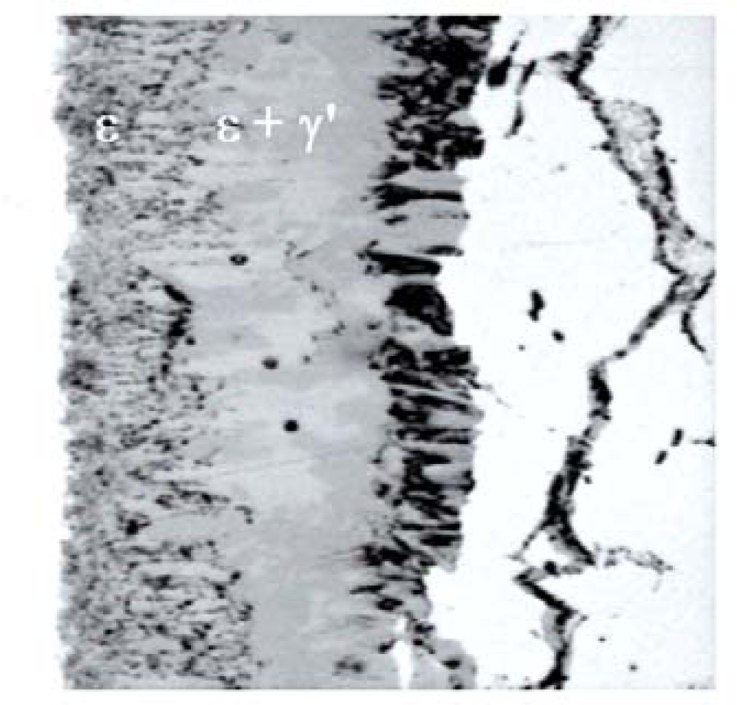
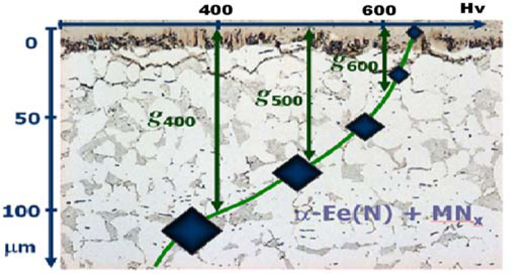
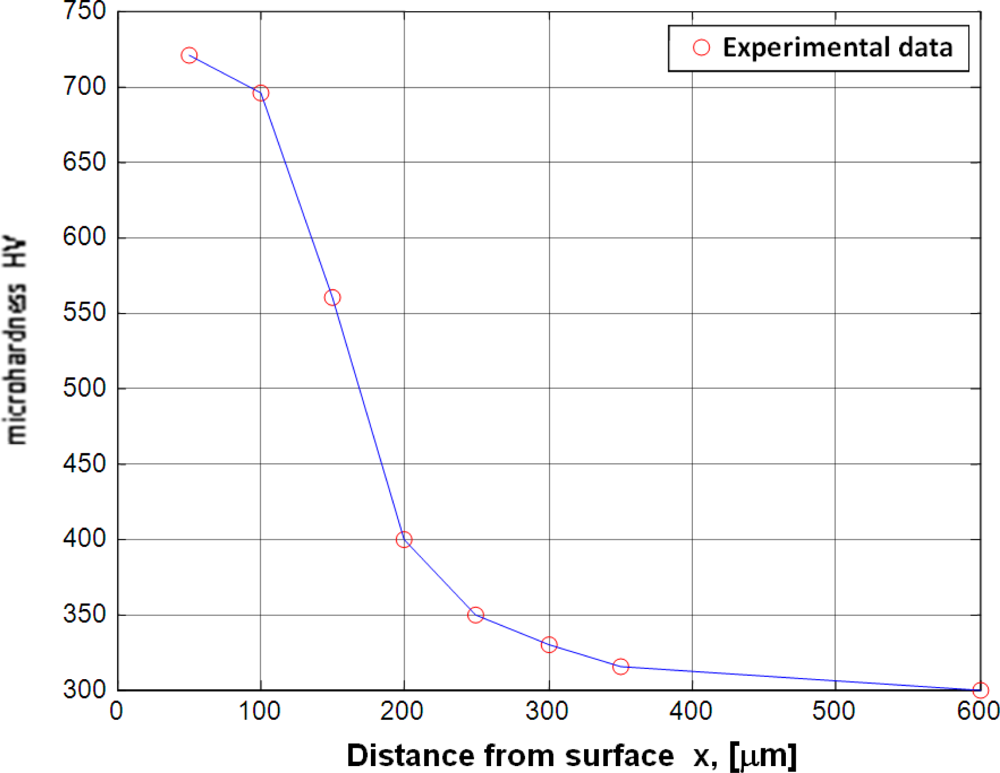
2. Structure of Nitrided Layer
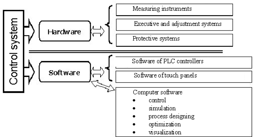
3. Control System
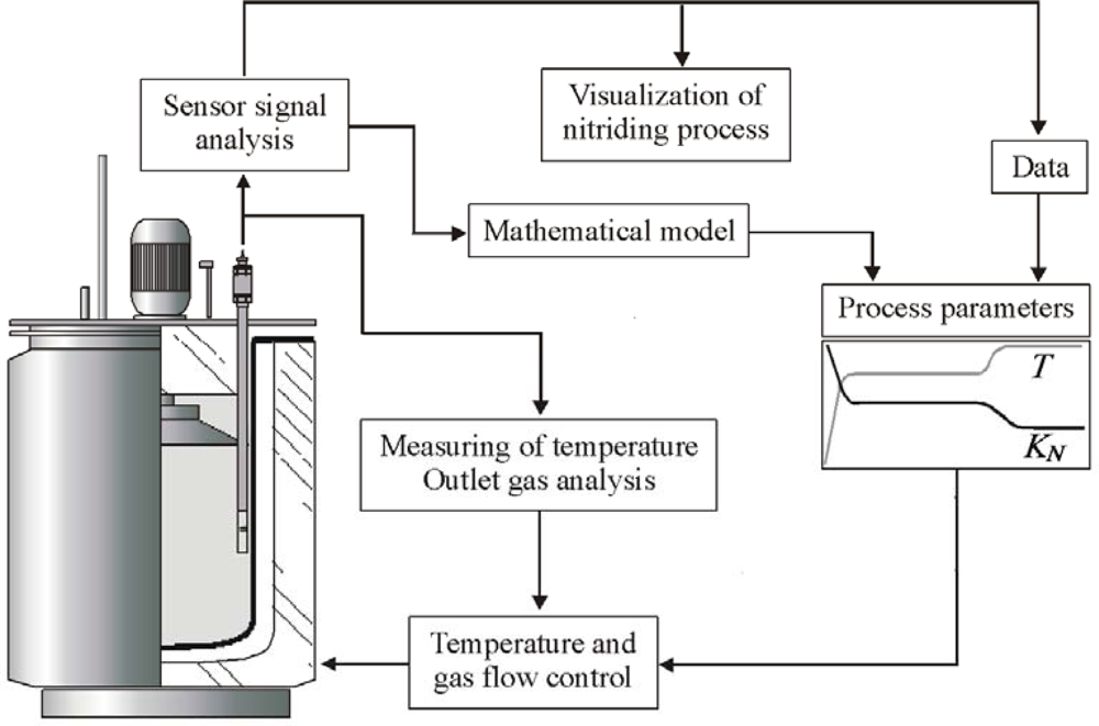
3.1. General Concept
3.2. Designing Block of Process Parameters
3.2.1. Guidelines
- the exceptionality rule, i.e., while designing the course of practically any nitriding process, it is necessary to use different values of the matrix of input parameters;
- the rule of focusing on the goals, i.e., achieving the foreseen properties of the layer with the application of the smallest possible number of technological operations, e.g., changes of the temperature, the nitrogen potential or the composition of the inlet atmosphere in the duration of the process;
- the rule of the limitation of preliminary information, i.e., too large a quantity of data at the start of designing results in an undesired complexity of the process;
- the rule of the use of knowledge databases, i.e., for the purpose of conclusions concerning the properties of the layer, reliable data is required concerning the processes realized, especially data concerning the correlation of the values of the material’s parameters before the process and the characteristics of the nitriding atmosphere with the data concerning the operating properties of the layer after the nitriding process, collected in the database and used for the generation of knowledge databases.
3.2.2. Models of the Process
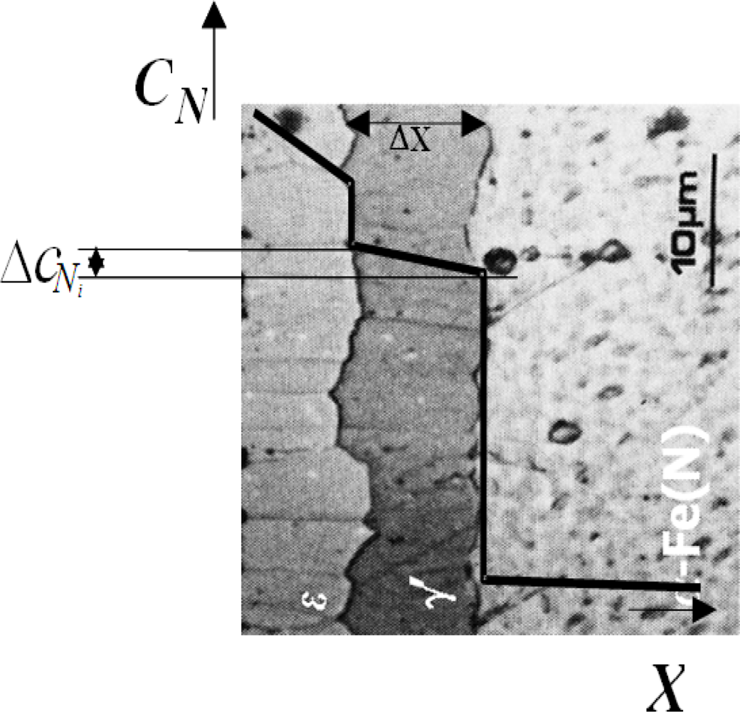
Analytical
- Δxi – thickness of ith phase in n-phase layer after process time t (for the nitrided layer, the maximum value n=3),
- ki– kinetic parameter of the growth of ith phase, the so-called constant of the parabolic growth of ith phase,
- t – process time.
- ki–kinetic parameters of the growth of ith and jth phase,
- Δci–difference of concentrations of the diffusing element on the border of ith phase.
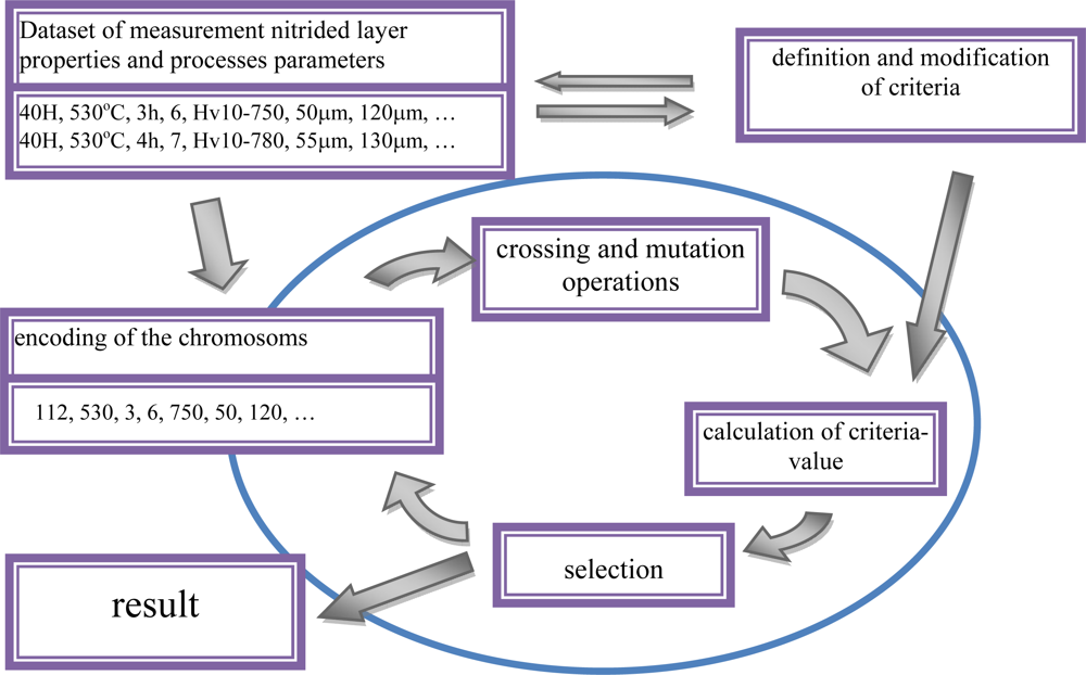
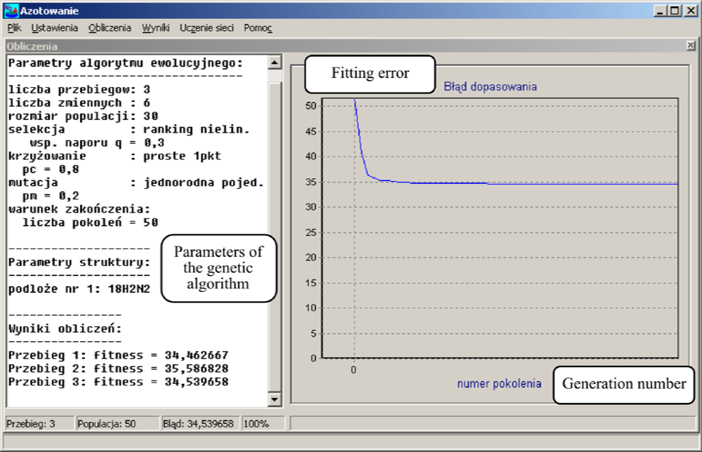
Statistical models based on artificial intelligence methods
- modelling of materials,
- simulations of nanocrystals and atomic/molecular clusters,
- optimization of metallurgical processes,
- designing/search for new materials with the required properties,
- supervision of the growth processes of single coats and multilayer coatings,
- an analysis of the physical and structural properties of thin-layer systems.
3.3. Visualization and Control of the Process
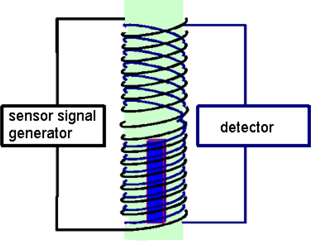
3.3.1. Selection of the Measuring Method
- Û0– voltage induced in the measuring winding when the coil is empty,
- η– coil filling factor,
- μr – relative magnetic permeability,
- μ̂sk – effective permeability: its introduction makes the value of the magnetic field intensity independent from the distance from the surface of the sample.

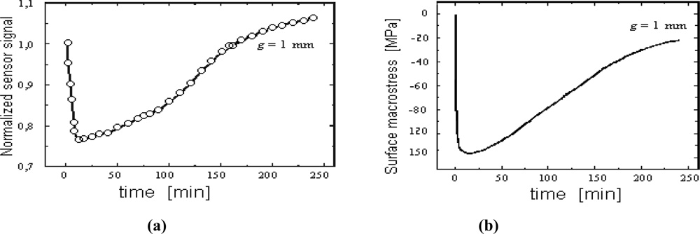
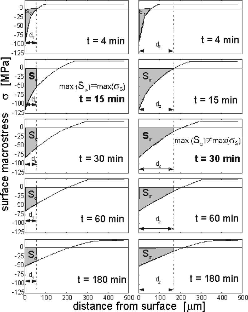
- σ(x,t) – macrostresses which are parallel to the surface, in x distance from the surface,
- β - Vegard constant,
- E - Young's modulus
- ν - Poisson constant,
- [N̄ (t)] - average nitrogen concentration in sample in t time of process,
- [N(x,t)] - surface nitrogen concentration in x distance from surface in t time of process.
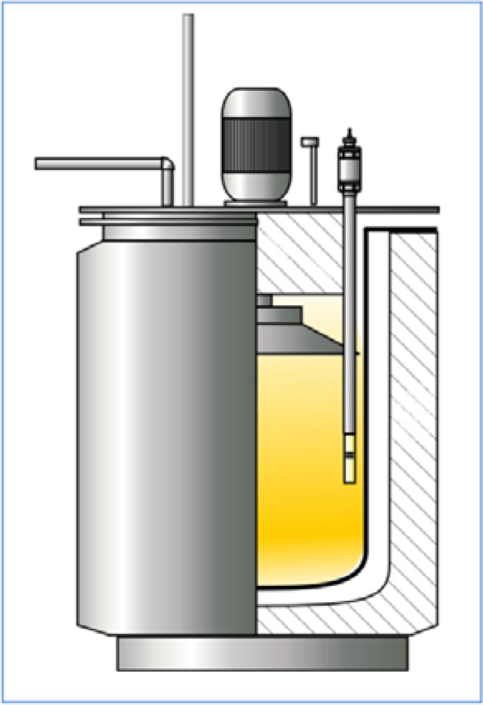
3.3.2. Design, Testing and Implementation of the Measuring Block
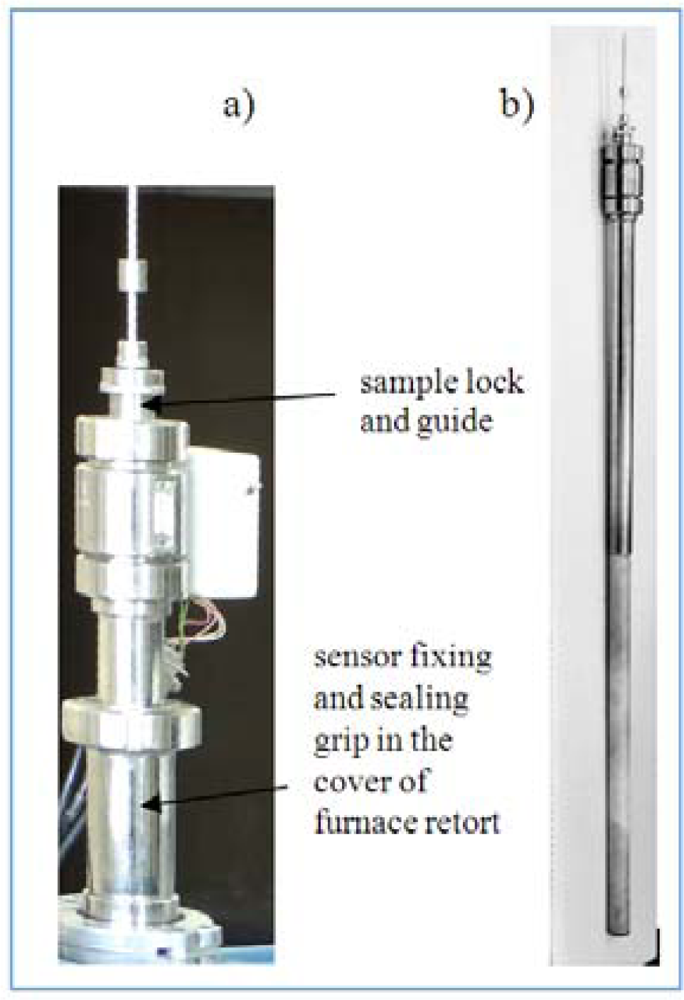
3.3.3. Design and Construction of Magnetic Sensor
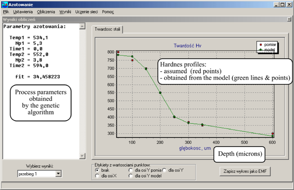
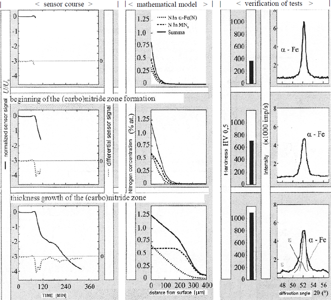
3.3.4. Development of Computer Models for in Situ Visualizations of the Layer Growth Kinetics
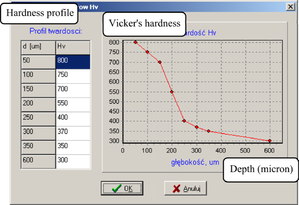
- dependencies were identified between the process parameters and the layer structure for an in situ visualization of the layer growth kinetics and for the control of the process which ensures an optimal layer due to its expected physical and chemical properties, and in particular its surface hardness as well as the thickness and the morphological composition;
- complementary cooperation was developed between the mathematical model and the indications of the magnetic sensor which registers in situ the formation of the nitrided layer.
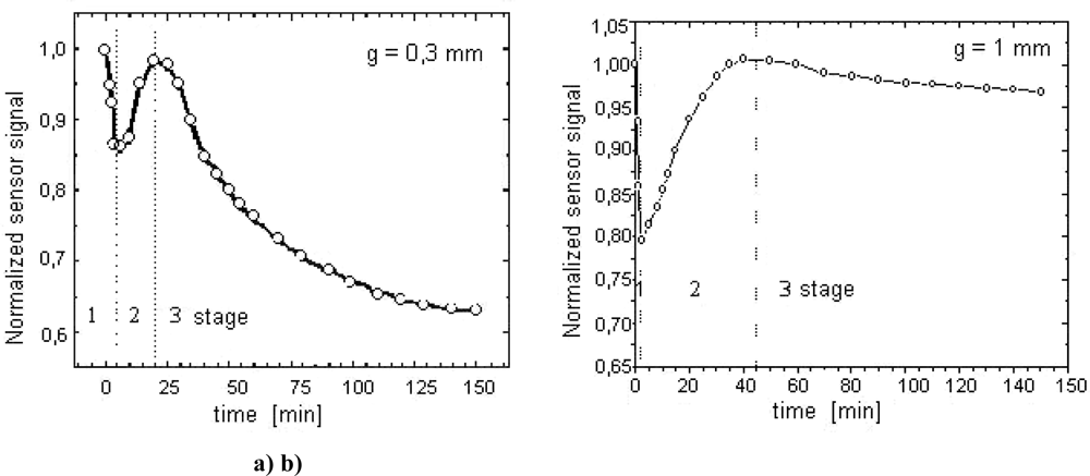
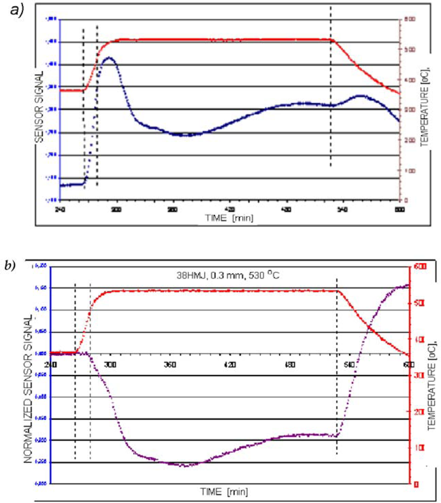
- an isolation of the background temperature from the signal registered with the magnetic sensor,
- an identification of the nucleation moment of nitrides,
- a detection of the further stages of the layer creation,
- a quantitative determination of the layer growth kinetics.
4. Discussion and Conclusions
References
- Malinov, S.; Sha, W. Software products for modelling and simulation in materials science. Comput. Mater. Sci 2003, 28, 179–198. [Google Scholar]
- Genel, K. Use of artificial neural network for prediction of ion nitrided case depth in Fe–Cr alloys. Mater. Design 2003, 24, 203–207. [Google Scholar]
- Zhecheva, A.; Malinov, S.; Sha, W. Simulation of microhardness profiles of titanium alloys after surface nitriding using artificial neural network. Surf. Coat. Tech 2005, 200, 2332–2342. [Google Scholar]
- Kumar, S.; Singh, R. A short note on an intelligent system for selection of materials for progressive die components. J. Mater. Process. Technol 2007, 182, 456–461. [Google Scholar]
- Lipiński, D.; Ratajski, J. Modeling of microhardness profile in nitriding processes using artificial neural network. Lect. Note Comput. Sci 2007, 4682, 245–249. [Google Scholar]
- Ratajski, J.; Ignaciuk, J.; Kwiatkowski, J.; Olik, R. The kinetics of nitriding layer growth on Fe-Cr and Fe-Ti alloys. Mater. Sci. Forum 1994, 163–165, 279–284. [Google Scholar]
- Ratajski, J.; Olik, R.; Liliental, W. New development trend: magnetic sensor to monitor nitride layer growth in process. Proceedings of the Second International Conference on Carburizing and Nitriding with Atmospheres, Cleveland, OH, USA, 1995; pp. 309–314.
- Ratajski, J. Monitoring nitride layer growth using magnetic sensor. Surf. Eng 2001, 17, 193–198. [Google Scholar]
- Ratajski, J.; Olik, R.; Baranov, A. Control system in situ of nitrided layer growth and deposited layer in PVD processes. Problemy Eksploatacji 2005, 2, 93–105. [Google Scholar]
- Ratajski, J.; Tacikowski, J.; Olik, R.; Suszko, T.; Łupicka, O. Intelligent control system for gaseous nitriding process. Metallurgia Italiana 2006, 6, 1b. [Google Scholar]
- Ratajski, J.; Suszko, T. Modelling of the nitriding process. J. Mater. Process. Technol 2008, 195, 212–217. [Google Scholar]
- Lehrer, E. Uber das Eisen-Wasserstoff-Ammoniak-Gleichgewicht. Z. Elektochem 1930, 26, 383–392. [Google Scholar]
- Somers, M.A.J.; Mittemeijer, E.J. Layer-growth kinetics on gaseous nitriding of pure iron: evaluation of diffusion coefficients for nitrogen in iron nitrides. Metall. Mater. Trans. A 1995, 26A, 57–74. [Google Scholar]
- Rozendaal, H.C.F.; Colijn, P.F.; Mittemeijer, E.J. Morphology, composition and residual stresses of compound layers of nitrocarburized iron and steels. Surf. Eng 1985, 1, 30–43. [Google Scholar]
- Langenhan, B.; Spies, H.J. Einfluss der nitrierbedingungen auf morphologie und struktur von verbindungsschichten auf vergutungsstahlen. Härterei-Techn. Mitt 1992, 47, 337–343. [Google Scholar]
- Zyśk, J.; Tacikowski, J.; Kasprzycka, E. Die Nitrierbarkeit auf ausgewahlter legierter Stahlen. Härterei-Techn. Mitt 1979, 34, 263–271. [Google Scholar]
- Prenosil, B. Gefuge der badnitrierten und in Ammoniakatmosphare mit Kohlenwasserstoffzusatz hergestellten Schichten. Härterei-Techn. Mitt 1965, 20, 41–49. [Google Scholar]
- Schwerdtfeger, K.; Grieveson, P.; Turkdogan, E.T. Growth rate of Fe4N on iron. Metall. Mater. Trans. A 1969, 245, 2461–2466. [Google Scholar]
- Mittemeijer, E.J.; Straver, W.T.M.; Van der Schaaf, P.J.; Van der Hoeven, J.A. The conversion cementite–ε nitride during the nitriding of Fe–C-alloys. Scripta Metall 1980, 14, 1189–1192. [Google Scholar]
- Mittemeijer, E.J.; Rozendaal, H.C.F.; Colijn, P.F.; Van der Schaaf, P.J.; Furnée, R.T. The microstructure of nitrocarburized steels. Proceedings of the Conf. on Heat Treatment; The Metal Society: London, UK, 1983; pp. 107–115. [Google Scholar]
- Ratajski, J.; Tacikowski, J.; Somers, M.A.J. Development of the compound layer of iron (carbo) nitrides during nitriding of steel. Surf. Eng 2003, 3, 87–93. [Google Scholar]
- Ratajski, J. Relation between phase composition of compound zone and growth kinetics of diffusion zone during nitriding of steel. Surf. Coat. Tech 2009, 203, 2300–2306. [Google Scholar]
- Dobrodziej, J.; Mazurkiewicz, A.; Ratajski, J.; Suszko, T.; Michalski, J. The methodology of fuzzy logic application in the modelling of thermodiffusive and PVD processes—Intelligent tools for support of designing in surface treatments. Proceedings of the International Federation of Heat Treatment and Surface Engineering (IFHTSE) Congress, Brisbane, Australia, 2007.
- Reti, T.; Czinege, I.; Frelde, I.; Grum, J.; Ju, D.Y. Selection of tools materials for cold forming operations using a computerized decision support system. Proceedings of the 17th International Federation of Heat Treatment and Surface Engineering (IFHTSE) Congress, Kobe, Japan, 2008.
- Burakowski, T.; Wierzchoń, T. Surface engineering of metals: principles, equipment, technologies; Taylor and Francis Group, LLC: Boca Raton, FL, USA, 2008. [Google Scholar]
- Dobrzański, L.A.; Madejski, J. Prototype of an expert system for selection of coatings for metals. J. Mater. Proc. Technol 2006, 175, 163–172. [Google Scholar]
- Mazurkiewicz, A. Mechanisms of knowledge transformation in the area of advanced technologies of surface engineering. In Incorporating Heat Treatment of Metals International Heat Treatment and Surface Engineering; IOM3: London, UK, 2007; Volume 1, pp. 108–113. [Google Scholar]
- Harada, A. The framework of Kansei engineering. Report of Modelling the Evaluation Structure of Kansei. University of Tsukuba: Tsukuba, Japan, 1997; pp. 49–55. [Google Scholar]
- Pitsch, W.; Houdremont, E. Ein Beitrug zum System Eisen-Stickstoff. Archiv für das Eisenhüttenwesen 1956, 27, 281–284. [Google Scholar]
- Gurov, K.P.; Kartaszkin, B.A.; Ugastie, J.E. Wzimnaja Diffuzija w Mnogofaznych Sistemach; Nauka: Moscow, Russia, 1981. [Google Scholar]
- Ratajski, J. Model of growth kinetics of nitrided layer in the binary Fe-N system. Zeitschrift fur Metallkunde 2004, 95, 23–29. [Google Scholar]
- Luger, G.F. Artificial intelligence and strategie for complex problem solving, 5th ed; Addison-Wesley: London, UK, 2005. [Google Scholar]
- Frazer, B.C. Magnetic structure of Fe4N. Phys. Rev 1958, 112, 751–754. [Google Scholar]
- Eickel, K.H.; Pitsch, W. Magnetic Property of Heksagonal Nitride Fe2,3 N. Phys. Stat. Sol 1970, 39, 121–131. [Google Scholar]
- Heptner, H.; Stroppe, H. Magnetische und magneinductive Werkstoffprüfung; VEB Deutscher Verlag für Grundstoffindustrie: Leipzig, Germany, 1965. [Google Scholar]
- Mittemeijer, E.J. The relation between macro-and microstresses and mechanical. Proceedings of the TMS-AIME Session on “Microstructural and Residual Stress Effects on the Properties of Case-Hardened steels”, Warrendale, PA, USA, 1984; pp. 161–187.
- Mittemeijer, E.J. Gitterverzerrungen in nitriertem Eisen und Stahl. Härterei-Techn. Mitt 1981, 36, 57–64. [Google Scholar]


| Steel | Number of samples | Range of parameters | ||||||||||
|---|---|---|---|---|---|---|---|---|---|---|---|---|
| EN | W.NR | PN | First degree | Second degree | ||||||||
| q-ty | T1[°C] | t1 [min] | KN | q-ty | T 2[°C] | t2 [min] | KN | |||||
| 1 | 18CrNi8 | 1.5920 | 18H2N2 | 10 | - | - | - | - | 10 | 530–570 | 120–780 | 3.2–6 |
| 2 | 0.2%C,1%Mn,1.2%Cr,0.1%Ti,0.3%Si | 18HGT | 85 | 20 | 480–580 | 120–270 | 1.15–30 | 85 | 480–580 | 25–3090 | 0.4–30 | |
| 3 | 20MnCr5 | 1.7147 | 20HG | 23 | - | - | - | - | 23 | 530–590 | 120–1920 | 2.75–4.5 |
| 4 | 25CrMo4 | 1.7218 | 25H3M | 10 | 4 | 530 | 240–270 | 5.25–11.5 | 10 | 530 | 120–3090 | 0.6–11.5 |
| 5 | ∼25CrMo4 | ∼1.7218 | 25H5M | 2 | 1 | 530 | 270 | 5.25–7 | 2 | 530 | 780–3090 | 0.8–5.25 |
| 6 | 30CrMoV9 | 1.7707 | 4340 | 32 | - | - | - | - | 32 | 530–590 | 120–1920 | 2.75–4.5 |
| 7 | 33CrMoV12-9 | 1.8519 | 33H3MF | 35 | 1 | 530–570 | 270 | 1.5–30 | 35 | 530–570 | 120–3090 | 0.8–30 |
| 8 | 35CrAlMo5 | 1.8506 | 35CrAlMo5 | 3 | - | - | - | - | 3 | 530–570 | 480 | 2.75–4.4 |
| 9 | 0.4%C,1%Mn,1.2%Cr,0.3%Ni,1.2%Si | 35HGSA | 2 | 2 | 540 | 360 | 20 | 2 | 540–550 | 3240 | 0.7–0.9 | |
| 10 | 34CrAl6 | 1.8504 | 34CrAl6 | 22 | - | - | - | - | 22 | 530–570 | 120–1920 | 3–4.5 |
| 11 | ∼35CrMo8 | ∼1.2312 | 36H3M | 6 | - | - | - | - | 6 | 550 | 720 | 1.5–30 |
| 12 | 38CrMoV21 | ∼1.2343 | ∼WCL | 32 | - | - | - | - | 32 | 530–590 | 120–1920 | 2.75–4.5 |
| 13 | 41CrAlMo7 | 1.8507 | 38HMJ | 44 | 19 | 480–580 | 120–480 | 1.1–30 | 44 | 480–580 | 25–3240 | 0.4–30 |
| 14 | 41Cr4 | 1.7035 | 40H | 43 | 3 | 500–570 | 60–270 | 1.5–30 | 43 | 500–570 | 120–3090 | 0.8–30 |
| 15 | 42CrMoV73 | 1.7741 | 40H2MF | 2 | 1 | 530 | 270 | 5.25–7 | 2 | 530 | 780–3090 | 0.8–5.25 |
| 16 | ∼42CrMo4 | ∼1.7225 | 40HM | 4 | - | - | - | - | 4 | 560–570 | 240–540 | 0.85–3.1 |
| 17 | 42CrMo4 | 1.7225 | 4140 | 15 | 2 | 530–570 | 270–450 | 0.85–7 | 15 | 530–570 | 120–3090 | 0.8–6.1 |
| 18 | 30CrMoV9 | 1.7707 | 4340 | 30 | 14 | 480–570 | 120–270 | 3.2–20 | 30 | 480–570 | 25–3090 | 0.8–20 |
| 19 | C45 | 1.0503 | 45 | 50 | 1 | 500–590 | 270 | 3–7 | 50 | 500–590 | 120–3090 | 0.8–4.75 |
| 20 | X40CrMoV511 | 1.2344 | WCLV (H13) | 1 | - | - | - | - | 1 | 500 | 360 | 5.1 |
| 21 | 1%C,0.7%Cr,0.7%Mn,0.6%Ni, 0.2%Si | IMPACTO | 8 | - | - | - | - | 8 | 530–570 | 120–720 | 3.2–6.1 | |
| 22 | 1.7%C,12%Cr,0.3%Mn,0.3%Ni | NC10 | 3 | - | - | - | - | 3 | 530–570 | 480 | 2.75–4.4 | |
| 23 | 42CrMo4 | 1.7225 | 4140 (SPS) | 8 | - | - | - | - | 8 | 530–570 | 120–720 | 3.2–6.1 |
| 24 | ∼HS6-5-2 | ∼1.3343 | SW3S2 | 5 | 5 | 530 | 240 | 9.25 | 5 | 530 | 120–1920 | 0.6 |
| 25 | X37CrMoV51 | 1.2343 | WCL | 16 | 6 | 530–570 | 240–270 | 1.5–30 | 16 | 530–570 | 120–3090 | 0.6–30 |
| TOTAL | 491 | 79 | 480–590 | 60–480 | 0.85–30 | 491 | 480–590 | 120–3090 | 0.4–30 | |||
©2010 by the authors; licensee Molecular Diversity Preservation International, Basel, Switzerland. This article is an open access article distributed under the terms and conditions of the Creative Commons Attribution license (http://creativecommons.org/licenses/by/3.0/)
Share and Cite
Ratajski, J.; Olik, R.; Suszko, T.; Dobrodziej, J.; Michalski, J. Design, Control and in Situ Visualization of Gas Nitriding Processes. Sensors 2010, 10, 218-240. https://doi.org/10.3390/s100100218
Ratajski J, Olik R, Suszko T, Dobrodziej J, Michalski J. Design, Control and in Situ Visualization of Gas Nitriding Processes. Sensors. 2010; 10(1):218-240. https://doi.org/10.3390/s100100218
Chicago/Turabian StyleRatajski, Jerzy, Roman Olik, Tomasz Suszko, Jerzy Dobrodziej, and Jerzy Michalski. 2010. "Design, Control and in Situ Visualization of Gas Nitriding Processes" Sensors 10, no. 1: 218-240. https://doi.org/10.3390/s100100218