Employing Measures of Heterogeneity and an Object-Based Approach to Extrapolate Tree Species Distribution Data

Abstract

Information derived from high spatial resolution remotely sensed data is critical for the effective management of forested ecosystems. However, high spatial resolution data-sets are typically costly to acquire and process and usually provide limited geographic coverage. In contrast, moderate spatial resolution remotely sensed data, while not able to provide the spectral or spatial detail required for certain types of products and applications, offer inexpensive, comprehensive landscape-level coverage. This study assessed using an object-based approach to extrapolate detailed tree species heterogeneity beyond the extent of hyperspectral/LiDAR flightlines to the broader area covered by a Landsat scene. Using image segments, regression trees established ecologically decipherable relationships between tree species heterogeneity and the spectral properties of Landsat segments. The spectral properties of Landsat bands 4 (i.e., NIR: 0.76–0.90 µm), 5 (i.e., SWIR: 1.55–1.75 µm) and 7 (SWIR: 2.08–2.35 µm) were consistently selected as predictor variables, explaining approximately 50% of variance in richness and diversity. Results have important ramifications for ongoing management initiatives in the study area and are applicable to wide range of applications.

1. Introduction

Information derived from high (i.e., <5m) spatial resolution remotely sensed data is critical for the effective management of forested ecosystems. However, fine spatial resolution remotely sensed data are typically expensive to acquire and process. In addition these data are normally limited in geographic coverage, thus limiting their applicability to landscape-level analysis. In contrast to high spatial resolution data sources, medium (i.e., 5–30 m) spatial resolution multispectral satellite imagery (e.g., Landsat) are readily and freely available, providing wall-to-wall landscape-level coverage [1,2]. However, Landsat data inherently lacks the spectral and spatial resolution required to meet all management needs and applications for most of the worlds’ forests. Thus, developing methods to extrapolate information derived from higher spatial resolution sensors to the much broader spatial extent provided by Landsat-like data has important ramifications for a variety of management goals [3].

One approach towards linking fine and moderate resolution remotely sensed data involves filtering the spatial resolution of fine-grained products to correspond with spatially coarser satellite imagery. A common approach towards filtering is through the majority, which determines the dominant value within a grid. While capable of determining dominance within predefined areas, majority calculations are problematic as they risk inflating the presence of common values while under-representing rarer categories [4]. As an alternative to conventional spatial filters such as the majority, measures of heterogeneity may be useful in degrading spatial resolution while maintaining important information content. Heterogeneity, defined here as the degree of spatial variation exhibited within an ecosystem, is known to impact the structure, function and distribution of biodiversity, and has proven relevant as an information source for forest restoration and conservation [5,6,7]. Despite their usefulness, measures of heterogeneity are typically calculated at somewhat arbitrary spatial extents within user-defined windows, thus limiting their applicability to forest management decisions made at varying scales. Heterogeneity measures could prove more applicable and representative if they corresponded with tangible, ecologically-relevant units (e.g., forest stands).

While pixel-based methods are typically employed when processing remotely sensed data, object-based methods, which emulate intuitive human interpretation, are better suited at identifying ecologically-relevant units [8,9]. Through an object-based approach, segmentation initially partitions an image into spectrally and spatially similar multi-pixel groups which correspond with definable landscape elements (e.g., forest stands) [8,10,11,12]. As opposed to arbitrarily defined spatial entities (i.e., pixels), image segments become the unit of analysis and are characterized according to their geometrical properties (e.g., size, shape) and underlying statistical values, allowing for definition of distinct classes to which all segments are assigned membership [10,13]. The utility of object-based methods for extrapolating fine spatial resolution products across broader areas represented by Landsat data has been established, but examples are few and limited to extrapolating LiDAR-derived metrics [13].

Here, we assessed the use of an object-based approach to extrapolate tree species heterogeneity beyond the localized extent of non-contiguous hyperspectral/LiDAR flight-lines to the broader extent of a Landsat satellite image. First, to justify our approach, we illustrate the shortcomings of coarsening tree species distribution data derived from airborne hyperspectral and LiDAR data using majority filtering. Next, a Landsat-5 Thematic Mapper image was segmented, providing wall-to-wall representation comprised of definable landscape elements (i.e., forest patches) instead of image pixels. Three measures of heterogeneity (i.e., richness, evenness and diversity) were then calculated for the extent of species-level data. The advantageousness of image segmentation is established through comparing representations of species heterogeneity at the scale of Landsat pixels versus variably sized image segments. Next, regression trees are used to determine the strength of relationships between the statistical and geometric properties of Landsat segments (i.e., independent predictor variables) and their corresponding tree species heterogeneity values (i.e., dependent response variables). Resulting statistical relationships were used to define rules and extrapolate species-level information to the extent of the British Columbian southern Gulf Islands (SGI). The applicability of these results to local ongoing management concerns and extension to other environs are also considered.

2. Experimental Section

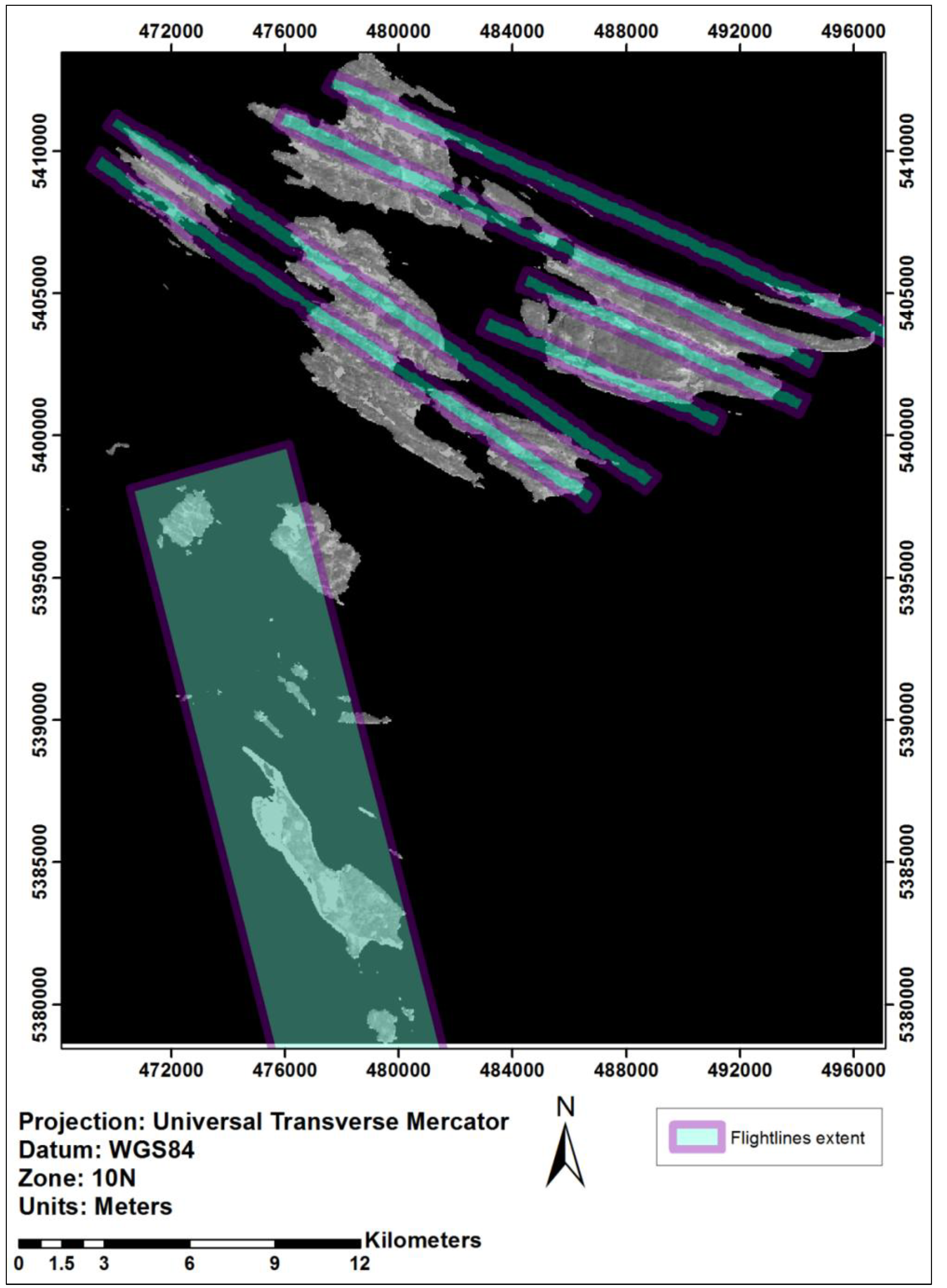
2.1. Study Area

The area of interest includes the Gulf Islands National Park Reserve (GINPR) and its surrounding lands in the SGI archipelago, in southwest BC, Canada, covering approximately 1050 km² (30 km east/west by 35 km north/south, centered at latitude 48.76° and longitude −123.18°), representing some of the province’s most diverse ecosystem assemblages [14] (Figure 1). Throughout the SGI, anthropogenic activities pose an ever-growing threat, making it one of the most ecologically at-risk regions in Canada [14]. Numerous forested ecosystem types and associated floral and faunal species are considered rare and/or at-risk [15]. Forested lands in the SGI are dominated by Pseudotsuga menziesii (Douglas-fir) and secondarily by Alnus rubra (red alder). Other common coniferous tree species, listed in their relative order of dominance, include Thuja plicata (Western red-cedar), Pinus contorta (lodgepole pine), Abies grandis (grand fir) and Tsuga heterophylla (Western hemlock). Additional typical broadleaf species include Arbutus menziesii (arbutus), Acer macrophylum (bigleaf maple), Populus balsamifera (black cottonwood), Quercus garryana (Garry oak) and Populus tremuloides (trembling aspen). Resulting from wide-spread harvesting, approximately 70% of forests are 40–80 years old, with tracts of mature stands 80–250 years (~25%), pole/sapling <40 years (~4%), and scattered late seral pockets >250 years in age (<1%) [16].

Figure 1. The British Columbian southern Gulf Islands as shown in the near infrared band of a Landsat-5 TM satellite image. The extent of hyperspectral/LiDAR flightlines are shown in green/purple.

Figure 1. The British Columbian southern Gulf Islands as shown in the near infrared band of a Landsat-5 TM satellite image. The extent of hyperspectral/LiDAR flightlines are shown in green/purple.

2.2. Data

2.2.1. Hyperspectral/LiDAR-Derived Tree Species Data

As described in [17], maps representing the distribution of 11 tree species were produced (at a 2 m spatial resolution) through the classification of fused airborne hyperspectral and LiDAR data, collected concurrently in mid-July, 2006. (Figure 2a provides an example of species data for a portion of the study area). Species maps provide detailed and accurate distribution information, with user’s and producer’s accuracies for most species ranging from >52%–95.4% and >63%–87.8%, respectively. However, this more accurate and detailed species-level data is limited to 23 non-contiguous flightlines, ~1 km wide and of variable length, covering approximately ~2800 ha [17].

Figure 2. For a portion of the study area: (a) 2 m tree species distribution data derived from fused airborne hyperspectral/LiDAR data. The background is area outside of the flightlines, represented by Landsat band 4 (NIR), (b) tree species richness calculated at a 30 m grain within the extent of airborne hyperspectral/LiDAR flightlines. The background is area outside of the flightlines, represented by Landsat band 4 (NIR), (c) Landsat-5 TM objects/segments falling within appropriate size thresholds and within the extent of airborne hyperspectral/LiDAR flightlines, and (d) 30 m tree species richness extrapolated beyond the extent of flightlines, wherein eight richness classes range from low to high.

Figure 2. For a portion of the study area: (a) 2 m tree species distribution data derived from fused airborne hyperspectral/LiDAR data. The background is area outside of the flightlines, represented by Landsat band 4 (NIR), (b) tree species richness calculated at a 30 m grain within the extent of airborne hyperspectral/LiDAR flightlines. The background is area outside of the flightlines, represented by Landsat band 4 (NIR), (c) Landsat-5 TM objects/segments falling within appropriate size thresholds and within the extent of airborne hyperspectral/LiDAR flightlines, and (d) 30 m tree species richness extrapolated beyond the extent of flightlines, wherein eight richness classes range from low to high.

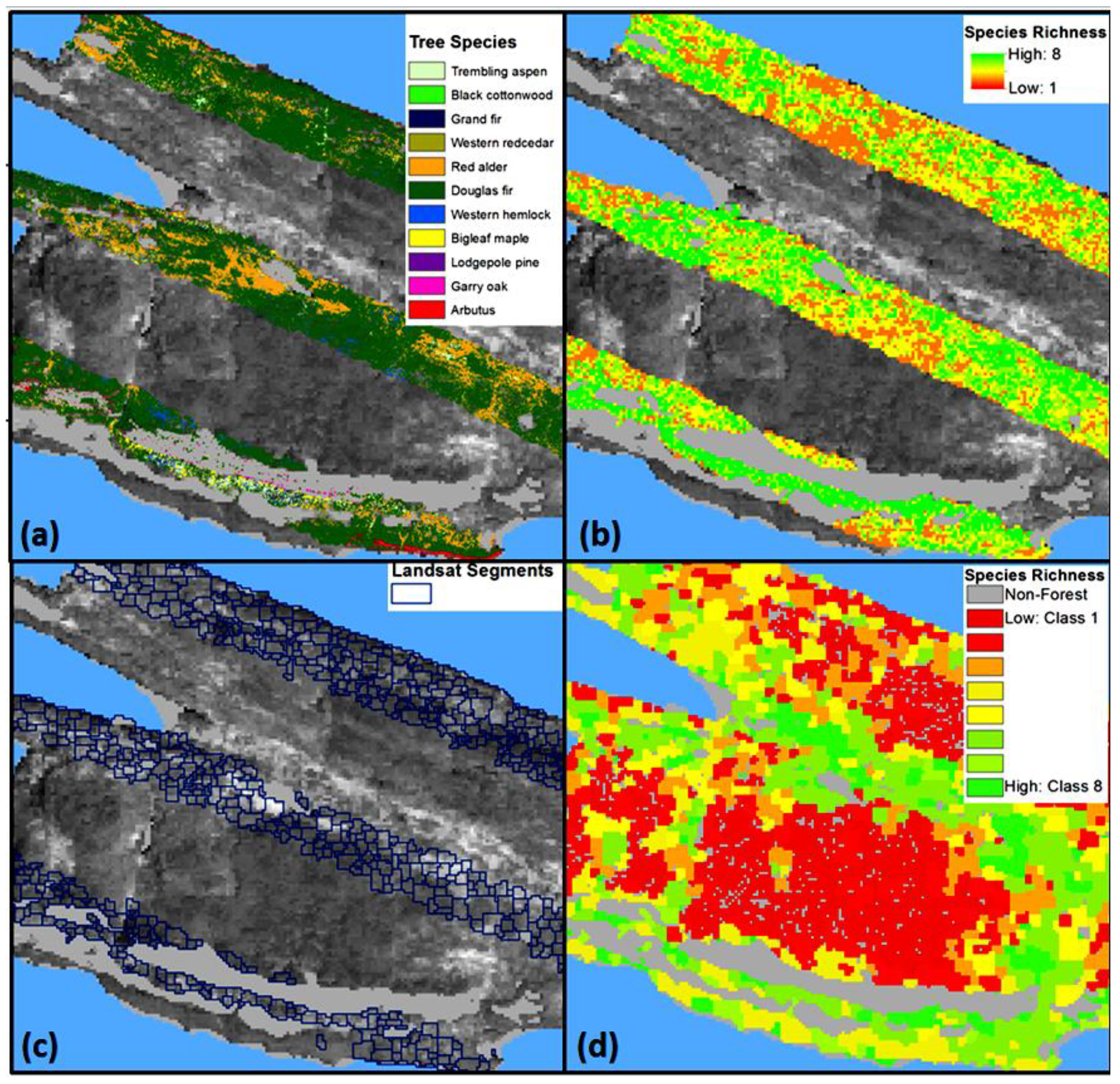
2.2.2. Tree Species Heterogeneity

To facilitate the extrapolation of species-level data to the extent of the SGI, three measures of heterogeneity were calculated within increasingly coarser windows from 10–100 m:

(1)

Tree species richness (R): the total number of species present

(2)

Simpson’s Index of diversity (D) as defined in [5]:

D = 1 /∑

Where pi represents the percentage cover of species i.

(3)

Tree species evenness (E) as defined in [5]:

E = D/R

As heterogeneity calculations were based on 11 species, richness could range from 1–11. Similarly, diversity could range from 1–11; wherein the greater the value, the more species classes present and the more evenly distributed the classes. Diversity could only match richness if all species types were equally represented. Evenness could range from 1/R to 1, with 1 occurring when all cover types were uniformly represented [5].

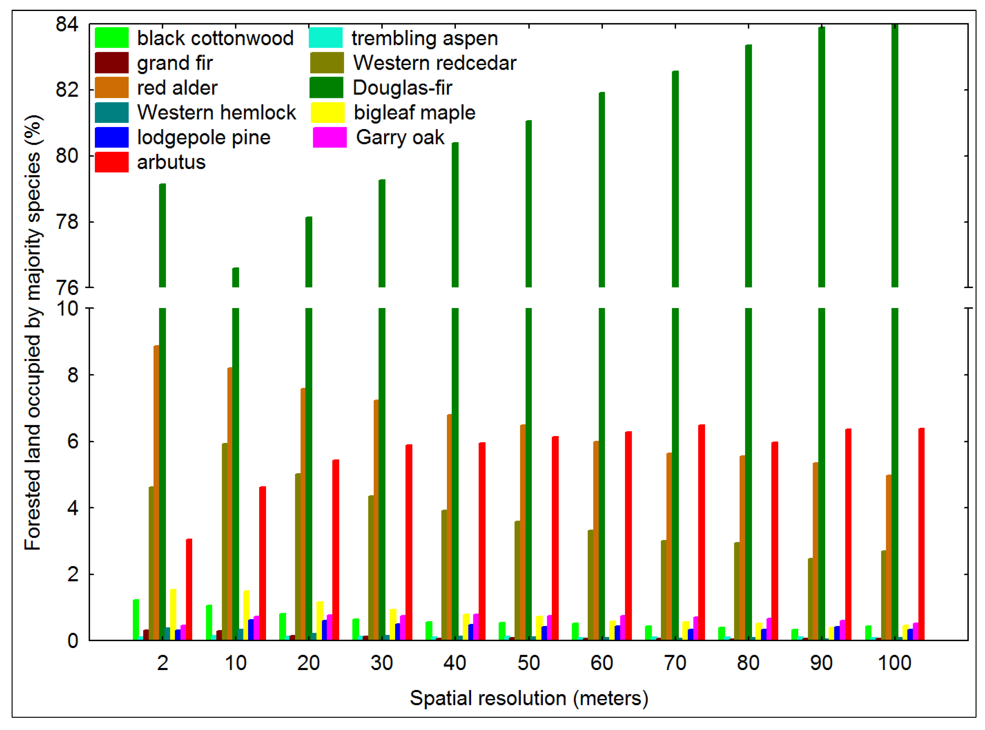
2.2.3. Tree Species Dominance

To facilitate a multi-scale comparison of the impact of coarsening species data using filtering (i.e., majority) versus heterogeneity measures, the majority (e.g., dominant) tree species was also determined within increasingly coarser windows, ranging from 10–100 m. Dominance was defined as the most common species within each window. As calculations were based on 11 possible species, the majority within each unit (i.e., pixel) at each scale was 1 of 11 possible classes.

2.2.4. Landsat Data

To facilitate the extrapolation of tree species heterogeneity, a broader scale landscape representation (coarser resolution and broader spatial extent) was provided by a Landsat-5 TM scene comprehensively covering the BC SGI (path: 47/row: 26) and encompassing the hyperspectral/LiDAR acquisition extent and timeframe (i.e., July, 2006). The image was delivered by MacDonald, Dettwiler and Associates (MDA) Ltd. precision georegistered, orthorectified, and resampled to a spatial resolution of 30 m, with an RMS error of 0.25. At-surface reflectance atmospheric correction was based upon the Cos(t) model [18], which estimated the effects of absorption by atmospheric gases and Rayleigh scattering and removed systematic atmospheric haze. All Landsat bands were masked to remove non-forest pixels.

2.3. Landsat Segmentation

To extract ecological units from the Landsat imagery [7] the image was segmented using eCognition Developer version 8.0.1 [12]. Objects or segments are formed by the creation of groups of similar homogenous pixels in a process called segmentation which merges pixels using a bottom-up, pair-wise, region-growing technique, which minimizes the heterogeneity within segments and maximizes their homogeneity [12]. Once segmented, objects can be characterized based on their inherent spectral and geometric properties, as well as by their location and position relative to other objects. Based on segment-level attributes, rules can be developed which define distinct classes to which all segments can be assigned membership [9].

2.4. Targeting Segment Features as Independent Variables

The characteristics of image segments (i.e., objects) considered for use in subsequent regression analyses included 19 aspects of geometry and 11 Landsat-layer specific statistics (Table 1). Landsat-layer statistics were derived from bands 1–5 and 7. This suite of 85 potential independent predictor variables was extracted from all Landsat segments completely within the extent of hyperspectral/LiDAR flightlines and imported into Statistica version 7.0 (StatSoft 2004) for analysis. Pearson-r correlation coefficients (p < 0.05) were calculated for all possible variable combinations. Based on coefficients of determination, an r² threshold of 0.85 eliminated redundant variables. Where two or more variables were highly correlated, emphasis was placed on the simpler and/or more ecologically relevant variable [7]. Extremely small and large (outlier) segments were eliminated based on minimum and maximum segment sizes of 0.54 (i.e., 6 pixels) and 2.7 ha (30 pixels), respectively.

Table 1. Aspects of segment geometry and segment-level spectral (i.e., Landsat) features considered as independent predictor variables. Segment-level statistics (i.e., layer summaries) were derived from bands 1–5 and 7.

Layer summaries	Geometry/shape
mean	area (meters)
standard deviation	area (pixels)
skewness	border length
minimum	length
maximum	length/width
mean inner border	volume
mean outer border	width
border contrast	asymmetry
contrast to neighbor pixels	border index
edge contrast to neighbor pixels	compactness
standard deviation to neighbor pixels	density
	elliptic fit
	main direction
	radius of largest enclosed ellipse
	radius of smallest enclosed ellipse
	rectangular fit
	roundness
	shape index

Table 1. Aspects of segment geometry and segment-level spectral (i.e., Landsat) features considered as independent predictor variables. Segment-level statistics (i.e., layer summaries) were derived from bands 1–5 and 7.

Layer summaries	Geometry/shape
mean	area (meters)
standard deviation	area (pixels)
skewness	border length
minimum	length
maximum	length/width
mean inner border	volume
mean outer border	width
border contrast	asymmetry
contrast to neighbor pixels	border index
edge contrast to neighbor pixels	compactness
standard deviation to neighbor pixels	density
	elliptic fit
	main direction
	radius of largest enclosed ellipse
	radius of smallest enclosed ellipse
	rectangular fit
	roundness
	shape index

2.5. Extraction of Segment-Level Heterogeneity Values (Dependent Variables)

Richness, diversity, and evenness values were determined for all Landsat derived segments within the extent of flightlines. Segment-level heterogeneity values initially facilitated comparison with pixel-level heterogeneity values, which aimed to establish the merits of image segmentation. In addition, segment-level heterogeneity values served as the response variables in regression tree analysis and subsequent extrapolation using an object-based approach.

2.6. Model Creation and Validation

Regression tree analyses [19,20] established which independent predictor variables exhibited relationships with and explained variance in species heterogeneity and further served to define rules for object-based extrapolation. Regression trees recursively partition a dataset into increasingly homogenous subsets, determining which of a candidate pool of independent variables (i.e., geometric and/or statistical properties of Landsat segments) can be used to predict a response (dependent) variable (i.e., tree species heterogeneity measures), and how much variance each predictor variable accounts for, which is the equivalent of an accuracy statement. Resulting trees supply a series of Boolean statements based on specific value thresholds of important predictor variables, ending in terminal nodes which define distinct classes, permitting a transparent, straightforward interpretation of results [10,21]. In addition to transparency, regression trees accommodate high dimensionality data and make no assumptions about input variables or their statistical distributions [10,22]. A regression tree was constructed to predict each measure of heterogeneity (i.e., richness, diversity, and evenness), wherein segment-level geometric properties and/or statistical summaries of Landsat data were the independent predictor variables. For each tree, rules defined the membership parameters for distinct classes of heterogeneity based on specific thresholds corresponding with specific predictor variables. K-fold cross-validation (K = 10) determined optimal tree size and accuracy for each tree [23], wherein explained variance measured how well each tree fit the data.

2.7. Extrapolation through an Object-Based Approach

Using the rules generated through regression tree analyses, all image segments were assigned memberships to richness, diversity, and evenness classes through an object-based approach, resulting in three coverages representing each measure of heterogeneity (i.e., richness, diversity, and evenness) for the extent of the BC SGI. As class assignment was based entirely on defined rules, the accuracy of resulting maps reflected the amount of variance explained by each associated regression tree, and therefore, additional accuracy assessment was not conducted. Using this transparent rule-based object-based approach avoided salt-and-pepper effects common to traditional pixel-based approaches [24], permitting more realistic final products. In addition, using segments instead of pixels as the unit of analysis reduced computational time by orders of magnitude [9].

3. Results

3.1. Impact of Majority Filtering in Tree Species Dominance

Increasingly coarser majority filters applied to the original 2 m species data (Figure 2a) (derived from and within the extent of hyperspectral/LIDAR flightlines changed the amount (%) of forested land occupied by each species (Figure 3) in five key ways, (1) the overall amount of forested land occupied by a species continuously decreased at each coarser spatial resolution, the most common scenario, impacting five species (i.e., black cottonwood, grand fir, red alder, Western hemlock and bigleaf maple), (2) the overall amount occupied increased, but eventually decreased, as demonstrated by trembling aspen and Western redcedar, (3) the amount of forested land occupied continuously increased, as exhibited by arbutus, (4) the amount of the forested land occupied initially decreased, but eventually increased, as seen with Douglas-fir, or (5) the amount fluctuated, trending towards an increase, but ending up approximately the same (i.e., lodgepole pine and Garry oak). Increasingly coarser spatial resolution typically resulted in an increase in the most dominant species (i.e., Douglas-fir), with decreases in rarer species (e.g., black cottonwood, trembling aspen, grand fir, Western hemlock, bigleaf maple). Coarsening to the spatial resolution of Landsat (i.e., 30 m) exaggerated the proportion of Douglas-fir, trembling aspen, Garry oak, lodgepole pine, arbutus and grand fir by 10, 25, 51, 69, 96 and 307%, respectively, while other species exhibited reductions of 5, 16, 38, 45 and 61% (i.e., Western redcedar, red alder, bigleaf maple, black cottonwood, Western hemlock, respectively).

Figure 3. The effect of coarsening spatial resolution on the amount (%) of forested land occupied by each species.

Figure 3. The effect of coarsening spatial resolution on the amount (%) of forested land occupied by each species.

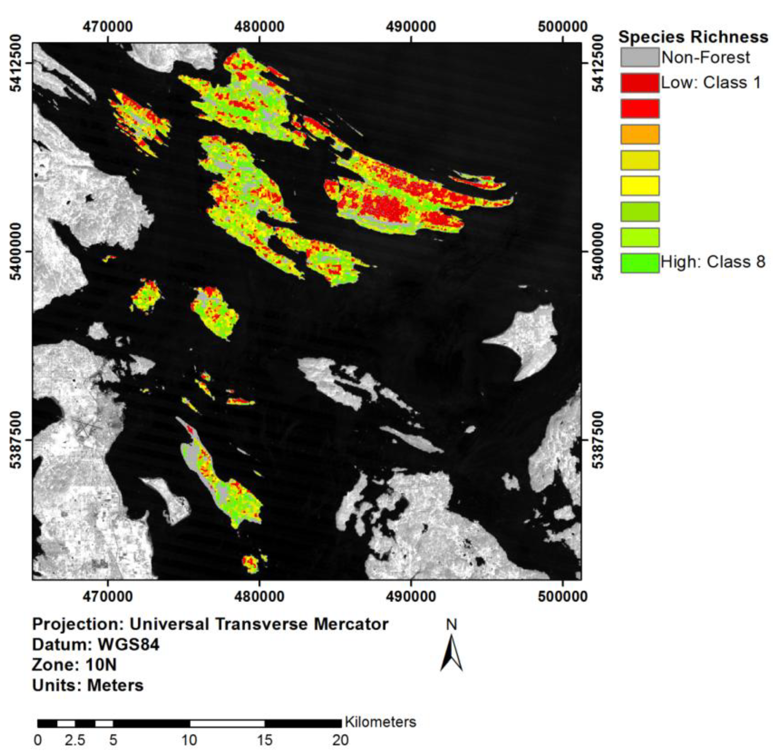
3.2. Tree Species Heterogeneity Calculated at the Pixel-Level

Calculating species heterogeneity at increasingly coarser spatial resolutions resulted in markedly different representations of richness, diversity and evenness (Table 2). Minimum species richness remained 1 regardless of resolution, while the maximum, mean and standard deviation steadily increased as spatial resolution increased from 10 (7, 1.48 and 0.71 respectively) to 100 m (11, 4.68 and 2.1, respectively). Minimum diversity also exhibited no change across scales, and similar to richness, the mean and standard deviation steadily increased as spatial resolution increased from 10 (1.25 and 0.44) to 100 m (1.62 and 0.67). Although maximum diversity fluctuated, it did not increase consistently. While maximum species evenness remained consistent at all scales, the minimum and mean consistently decreased as spatial resolution increased from 10 (0.31 and 0.9) to 100 m (0.12 and 0.42).

Table 2. The effect of coarsening spatial resolution (i.e., pixel size in meters) on three measures of tree species heterogeneity (i.e., richness, diversity, and evenness).

Spatial Resolution	Heterogeneity	Minimum	Maximum	Mean	Standard deviation
10	Richness	1	7	1.48	0.71
	Diversity	1	5.45	1.25	0.44
	Evenness	0.31	1	0.9	0.16
20	Richness	1	9	2.04	1.08
	Diversity	1	6.17	1.4	0.56
	Evenness	0.21	1	0.77	0.22
30	Richness	1	10	2.5	1.33
	Diversity	1	5.88	1.48	0.62
	Evenness	0.19	1	0.67	0.25
40	Richness	1	9	2.94	1.5
	Diversity	1	5.61	1.52	0.64
	Evenness	0.16	1	0.6	0.24
50	Richness	1	10	3.33	1.64
	Diversity	1	5.86	1.55	0.65
	Evenness	0.14	1	0.55	0.24
60	Richness	1	10	3.67	1.76
	Diversity	1	5.83	1.57	0.66
	Evenness	0.13	1	0.51	0.24
70	Richness	1	10	3.96	1.86
	Diversity	1	5.56	1.59	0.67
	Evenness	0.13	1	0.48	0.24
80	Richness	1	11	4.21	1.95
	Diversity	1	5.83	1.6	0.67
	Evenness	0.13	1	0.45	0.23
90	Richness	1	10	4.45	2.02
	Diversity	1	6.19	1.61	0.67
	Evenness	0.12	1	0.44	0.23
100	Richness	1	11	4.68	2.1
	Diversity	1	5.69	1.62	0.67
	Evenness	0.12	1	0.42	0.23

Table 2. The effect of coarsening spatial resolution (i.e., pixel size in meters) on three measures of tree species heterogeneity (i.e., richness, diversity, and evenness).

Spatial Resolution	Heterogeneity	Minimum	Maximum	Mean	Standard deviation
10	Richness	1	7	1.48	0.71
	Diversity	1	5.45	1.25	0.44
	Evenness	0.31	1	0.9	0.16
20	Richness	1	9	2.04	1.08
	Diversity	1	6.17	1.4	0.56
	Evenness	0.21	1	0.77	0.22
30	Richness	1	10	2.5	1.33
	Diversity	1	5.88	1.48	0.62
	Evenness	0.19	1	0.67	0.25
40	Richness	1	9	2.94	1.5
	Diversity	1	5.61	1.52	0.64
	Evenness	0.16	1	0.6	0.24
50	Richness	1	10	3.33	1.64
	Diversity	1	5.86	1.55	0.65
	Evenness	0.14	1	0.55	0.24
60	Richness	1	10	3.67	1.76
	Diversity	1	5.83	1.57	0.66
	Evenness	0.13	1	0.51	0.24
70	Richness	1	10	3.96	1.86
	Diversity	1	5.56	1.59	0.67
	Evenness	0.13	1	0.48	0.24
80	Richness	1	11	4.21	1.95
	Diversity	1	5.83	1.6	0.67
	Evenness	0.13	1	0.45	0.23
90	Richness	1	10	4.45	2.02
	Diversity	1	6.19	1.61	0.67
	Evenness	0.12	1	0.44	0.23
100	Richness	1	11	4.68	2.1
	Diversity	1	5.69	1.62	0.67
	Evenness	0.12	1	0.42	0.23

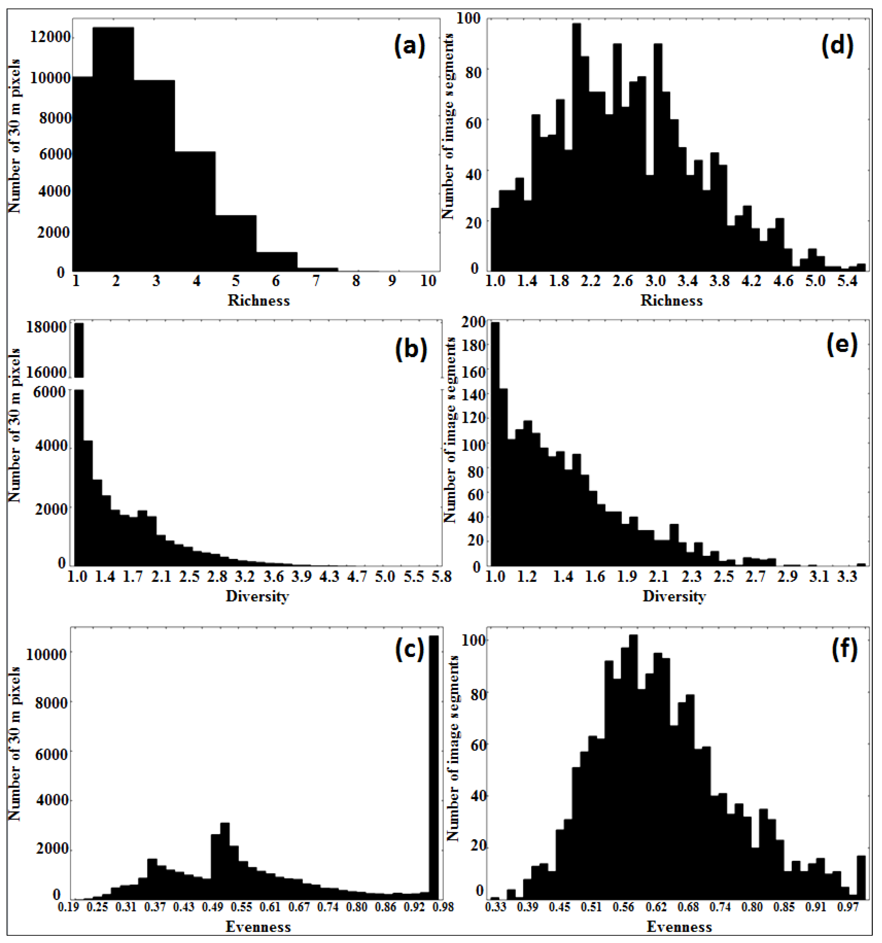
3.3. Tree Species Heterogeneity: Comparison of Pixel- To Segment-Level

Segmentation resulted in 8190 segments of which 1818 were within the area of the hyperspectral/LiDAR flightlines (example segments are shown for a portion of the study area in Figure 2c). Segment size ranged from 0.54–2.7 ha, averaging 1.23 ha (±0.54). Table 3 compares average pixel with segment-level statistics. Focusing on the spatial resolution of Landsat (i.e., 30 m), Figure 2b provides an example of tree species heterogeneity (richness) calculated within the extent of hyperspectral/LiDAR flightlines for a portion of the study area. At this scale, no single segment contained all 11 species classes, with richness values ranging from 1–10 (Table 3, Figure 4a), however, richness averaged 2.60 (±1.33, 1 standard deviation). Similarly, no single pixel contained species with equal or somewhat equal distribution, as diversity ranged from 1.00–5.90, averaging 1.48 (±0.61) (Table 3, Figure 4b). Species evenness ranged from 0.19–1.00, averaging 0.66 (±0.24) (Table 3, Figure 4c).

Table 3. Comparison of descriptive statistics for tree species heterogeneity.

	Pixel	Segment	Pixel	Segment	Pixel	Segment
	Richness		Diversity		Evenness
Minimum	1	1	1	1	0.19	0.33
Maximum	10	5.58	5.9	3.45	1	1
Mean	2.6	2.66	1.48	1.48	0.66	0.64
Standard deviation	1.33	0.9	0.61	0.4	0.24	0.12

Table 3. Comparison of descriptive statistics for tree species heterogeneity.

	Pixel	Segment	Pixel	Segment	Pixel	Segment
	Richness		Diversity		Evenness
Minimum	1	1	1	1	0.19	0.33
Maximum	10	5.58	5.9	3.45	1	1
Mean	2.6	2.66	1.48	1.48	0.66	0.64
Standard deviation	1.33	0.9	0.61	0.4	0.24	0.12

Figure 4. Comparison of frequency distribution for tree species heterogeneity values based on 30 m pixels for richness (a), diversity (b) and evenness (c), and for image objects for richness (d), diversity (e) and evenness (f).

Figure 4. Comparison of frequency distribution for tree species heterogeneity values based on 30 m pixels for richness (a), diversity (b) and evenness (c), and for image objects for richness (d), diversity (e) and evenness (f).

For evenness, the maximum value (i.e., 1) occurred most often, representing pixels for which all species present were equally distributed. In contrast, at the segment-level, while minimum species richness remained 1, maximum richness was substantially more (i.e., 5.58 vs. 10.00) (Table 3, Figure 4a,d). Similarly, while minimum species diversity values were 1 at both scales, maximum segment diversity was 1.45 greater (i.e., 3.45 vs. 5.90) (Table 3, Figure 4b,e). For species evenness, maximum values were the same at both scales, however, minimum values were typically higher for segments. Mean values for all three metrics were similar if not the same at both scales, whereas standard deviations were typically lower for segments (Table 3, Figure 4c,f).

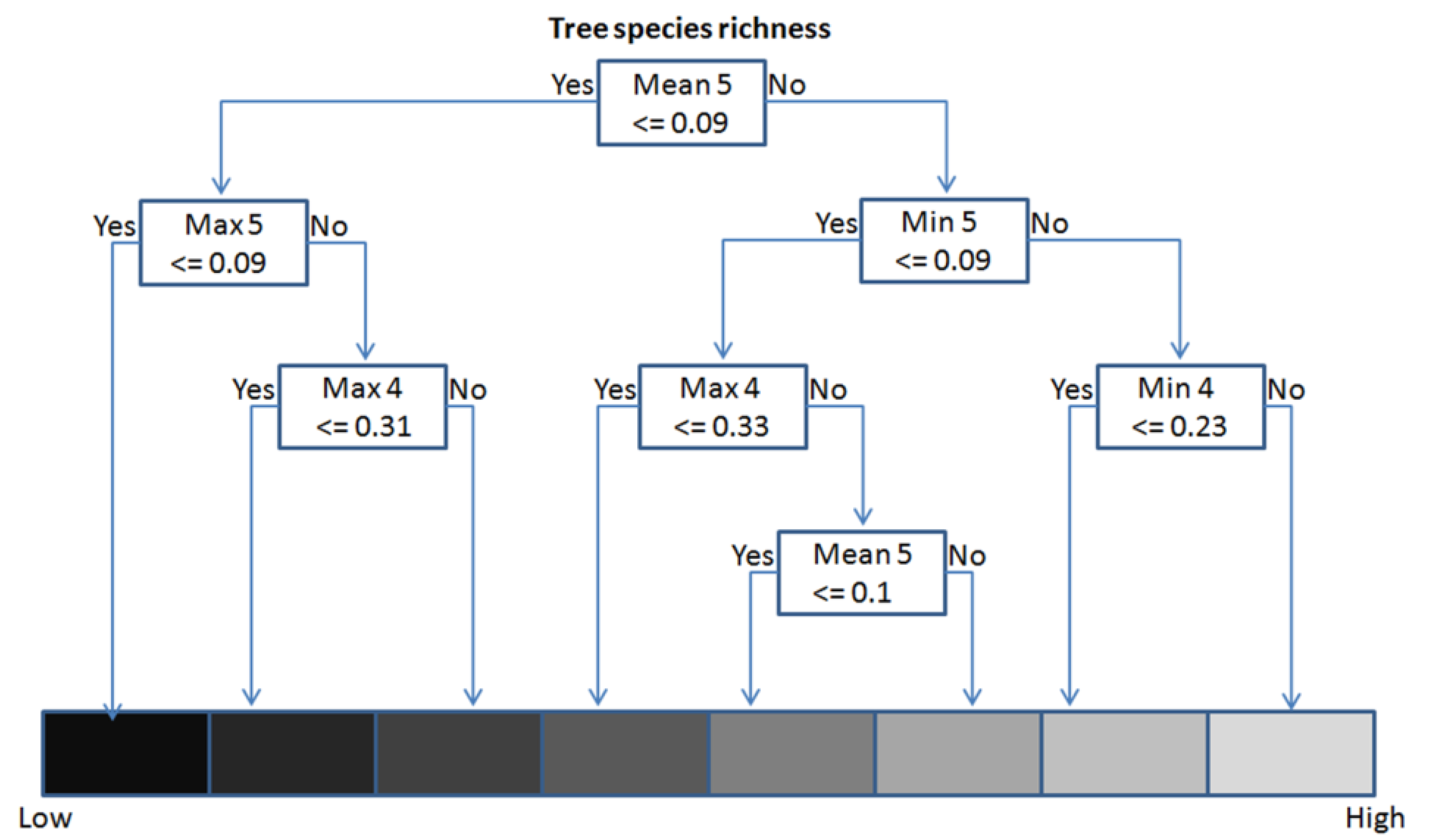
3.4. Model Definition and Validation (Regression Tree Analysis)

Based on pair-wise Pearson’s correlation coefficients, ecological significance, and preliminary relationship assessment (i.e., scatter-plots), 16 metrics representing the statistical properties of Landsat segments out of a total pool of 85 potential variables were retained for analysis as potential independent variables (Table 4). No geometric properties of Landsat segments passed the initial pre-selection criteria for consideration as potential variables. Regression tree analysis identified eight of 16 which partially explained variance within dependent response variables (i.e., measures of heterogeneity) (Table 4). For species richness, eight distinct classes were identified based on the statistical properties of Landsat bands 4 (NIR) and 5 (SWIR), with generated decision rules accounting for 48.9% of variance. Similar to richness, for diversity, a final model with eight terminal nodes was generated using bands 4 and 5, explaining 43.9% of variance. The importance of band 7 (SWIR) was also apparent. For species evenness, six terminal nodes defined rules which also indicated bands 4 and 5 were important predictors, however, as compared with diversity and richness, much less variance was explained (i.e., 22%).

Using richness as an example, Figure 5 shows the structure of a regression tree, wherein each node represents a decision rule generated based on the spectral reflectance properties of vegetation in the NIR and/or SWIR. The initial split was on average band 5 values of 0.09 (% reflectance/100), partitioning the image into segments with higher (>0.09) or lower (≤0.09) richness values. Segments with higher richness values were further partitioned based on minimum band 4 and 5 values, maximum band 4 values, and mean 5 band values. The highest richness classes were associated with minimum band 5 and 4 values of >0.09 and 0.23, respectively, isolating segments with the highest minimum reflectance thresholds for these spectral regions. In contrast, segments with lower richness values were further partitioned based on maximum values of 0.09 and 0.31 for bands 5 and 4, respectively. Segments with the least richness had maximum band 5 values ≤0.09, whereas segments with maximum 4 values >0.31 had slightly higher values.

Table 4. Independent variables representing spectral (i.e., Landsat) statistics, considered for and selected in regression tree analyses. An ‘x’ represents variables considered for but not selected in analyses, whereas an ‘xx’ represents selected variables. All other variables were not considered for analysis, based on pair-wise Pearson’s correlation coefficients (p < 0.05), a lack of ecological significance, and/or preliminary relationship assessment (i.e., scatterplot analysis).

	Wavelength (µm)	Minimum (Min)	Maximum (Max)	Mean	Standard deviation (Stdev)	Mean inner border (MIB)
band 1	0.45–0.52	x
band 2	0.52–0.60	x			x
band 3	0.63–0.69	x			x
band 4	0.76–0.90	xx	xx		x	xx
band 5	1.55–1.75	xx	xx	xx	xx	x
band 7	2.08–2.35	xx			x

Table 4. Independent variables representing spectral (i.e., Landsat) statistics, considered for and selected in regression tree analyses. An ‘x’ represents variables considered for but not selected in analyses, whereas an ‘xx’ represents selected variables. All other variables were not considered for analysis, based on pair-wise Pearson’s correlation coefficients (p < 0.05), a lack of ecological significance, and/or preliminary relationship assessment (i.e., scatterplot analysis).

	Wavelength (µm)	Minimum (Min)	Maximum (Max)	Mean	Standard deviation (Stdev)	Mean inner border (MIB)
band 1	0.45–0.52	x
band 2	0.52–0.60	x			x
band 3	0.63–0.69	x			x
band 4	0.76–0.90	xx	xx		x	xx
band 5	1.55–1.75	xx	xx	xx	xx	x
band 7	2.08–2.35	xx			x

Figure 5. Decision rules generated through regression tree analysis, wherein tree species richness was the dependent response variable, and segment-level spectral properties of Landsat data were selected as independent predictor variables. Landsat values relate to the statistical properties of reflectance values in specific portions of the electromagnetic spectrum (i.e., bands).

Figure 5. Decision rules generated through regression tree analysis, wherein tree species richness was the dependent response variable, and segment-level spectral properties of Landsat data were selected as independent predictor variables. Landsat values relate to the statistical properties of reflectance values in specific portions of the electromagnetic spectrum (i.e., bands).

3.5. Extrapolation through an Object-Based Approach

Based on generated decision rules, three maps were produced representing tree species richness, diversity and evenness for the extent of the BC SGI. An example of extrapolated richness is shown for a portion of the study area in Figure 2d, whereas Figure 6 presents extrapolated richness for the extent of the SGI, as represented by a Landsat-5 TM scene.

Figure 6. Tree species richness, derived from 2 m spatial resolution species distribution maps extrapolated to the extent of the British Columbian Southern Gulf Islands. The background image is Landsat band 4 (NIR) coverage.

Figure 6. Tree species richness, derived from 2 m spatial resolution species distribution maps extrapolated to the extent of the British Columbian Southern Gulf Islands. The background image is Landsat band 4 (NIR) coverage.

4. Discussion

4.1. Tree Species Heterogeneity Compared with Majority Filtering

Results suggest that heterogeneity measures were a more appropriate technique for coarsening the spatial resolution of detailed airborne data than simple majority filtering. While heterogeneity measures cannot discriminate how much of a sub-category type (e.g., species) actually exists within a predefined area, and increasingly coarser spatial resolutions can alter information content, their use resulted in less severe information alteration then majority filtering. Given the established links of heterogeneity with ecological structure and function, employing heterogeneity measures holds promise in coarsening finer spatial resolution products as a precursor to extrapolation.

4.2. Tree Species Heterogeneity: Comparison of Pixel to Segment-Level

There were notable differences in heterogeneity values at the scale of Landsat (i.e., 30 m pixels) versus the variable scale of segments. Owing to their multi-pixel nature, segments exhibited less range in richness, diversity and evenness values. Pixels with high values were typically reduced within larger segments, thus reducing their overall range. In addition, at the pixel-level, there was a markedly higher frequency of low richness and diversity values, and high/maximum evenness values. This discrepancy is partly explained by the dominance of Douglas-fir, which occupies the majority of the forested landscape, regardless of scale (i.e., 79.1%, at 2 m, 79.2%, at 30 m, 84%, at 100 m). If only one species occupies a pixel, it is still assigned a maximum evenness score, whereas pixels occupied by fewer species receive lower richness and diversity scores. While many segments were dominated by Douglas-fir, other species were typically also present. In addition, very few segments were completely occupied by a single species, even Douglas-fir. In aggregate, differences in values imply that information loss and/or manipulation does occur with consideration at the segment versus pixel scale, however, these changes are required to represent the landscape based on definable landscape elements (e.g., forest stands) as opposed to arbitrary units (e.g., image pixels) [9,25]. In addition, the impacts of coarsening using heterogeneity measures are not as severe as they would be if employing standard filtering procedures (i.e., majority).

4.3. Regression Tree Results

For all three heterogeneity measures, independent explanatory variables were consistently Landsat bands 4, 5 or 7, demonstrating the importance of vegetation’s reflective properties in certain NIR and SWIR spectral regions. In band 4 (i.e., NIR: 0.76–0.90 micrometers (µm)), reflectance is primarily regulated by internal leaf structure [26], whereas in bands 5 (i.e., SWIR: 1.55–1.75 µm) and 7 (SWIR: 2.08–2.35 µm), reflectance is much lower than in the NIR and dominated by the presence of moisture and various canopy biochemicals (e.g., protein, lignin, cellulose) [27,28]. Established associations between vegetation and spectral reflectance in the NIR and SWIR permit informed and meaningful ecological characterization of image segments. Using richness as an example, segments with band 5 values >0.09 exhibited higher values, meaning they contained multiple tree species. Multi-species segments are more prone to host coniferous and broadleaved species. Due to the comparatively higher levels of biomass associated with broadleaves, segments containing broadleaved species should exhibit higher SWIR reflectance values. Therefore, segments with higher SWIR values were more likely to be richer and contain broadleaved tree species. In addition to high SWIR values, highest richness classes were also associated with highest NIR values. Similar to the SWIR, healthy broadleaves exhibit higher reflectance than conifers in the NIR. Therefore, because segments with higher richness values are more likely to contain broadleaved species, they will typically exhibit higher SWIR and NIR reflectance. Exceptions to these associations could include, (1) segments containing trees exhibiting signs of stress and/or (2) a disproportionate dominance of multi-specied segments known to contain none or few broadleaved trees, however, previous studies [17,29] indicate these exceptions are rare in the SGI.

4.4. Implications of Object-Based Extrapolation

Regression rules generated based on specific reflective aspects of NIR and SWIR bands transparently facilitate the extrapolation of heterogeneity to the extent of the BC SGI by guiding the assignment of membership into distinct classes for all image segments. For managers in the SGI, object-based extrapolation results supply broad scale tree species heterogeneity information. This information can aid a range of ongoing restoration and conservation tasks [29,30]. While similar heterogeneity measures could be calculated on a per-unit basis from aerial photo attributes, as detailed in [29], our heterogeneity measures were derived from comparatively more detailed and accurate tree species distribution information (i.e., 2 m spatial resolution maps derived from airborne hyperspectral/LiDAR data). In addition, even after factoring in the time associated with parameterization, image segmentation and extrapolation require significantly less time and labor than conventional methods. Aerial photo interpretation also requires non-automatable manual labor, which relies on increasingly less available skilled analysts [11], and therefore, once established, final scaling parameters permit transparent, timely replication. As such, established relationships could form the basis for extrapolation to archival, and/or newly acquired Landsat scenes, facilitating historic mapping and long-term monitoring of landscape-level tree species heterogeneity.

In terms of costs, it has previously been demonstrated that the acquisition, processing and interpretation costs of hyperspectral and LiDAR data in the SGI are half the price of aerial photographs [30]. While this will not be the case everywhere, the costs of these technologies have been found comparable in numerous and variable environs (Wulder et al., 2008) [31]. Within this monetary context, it is important to note that the advanced airborne data used in this study were collected in transects vs. the wall-to-wall acquisition of aerial photographs. However, relationships with Landsat segments facilitated low-cost extrapolation from the limited extent of detailed airborne measurements.

5. Conclusions

Image segmentation, regression tree analyses provided a transparent and effective means for extrapolating certain measures of tree species heterogeneity beyond the boundaries of non-contiguous hyperspectral and LiDAR flightlines to the wall-to-wall coverage provided by a Landsat scene. While heterogeneity measures cannot discriminate how much of a species exists within a predefined area, and increasingly coarser spatial resolutions can alter information content, their use involved less severe information alteration then majority filtering. This finding has important ramifications, given the common use of filters such as the majority for coarsening fine spatial resolution environmental data as a pre-cursor to extrapolation. At the segment scale, calculating heterogeneity results in definable forest units containing tangible heterogeneity values, which as units of analyses, have pertinence to a variety of ongoing and/or potential management initiatives. Image segmentation permits this comparatively superior landscape representation, and based on transparent relationships with spectral properties of Landsat data deduced through regression tree analyses, an object-based approach permits extrapolation, resulting in unprecedented heterogeneity information for the extent of the SGI explaining nearly half the variance in tree species richness and diversity.

In the SGI, the spectral properties of Landsat bands 4 (i.e., NIR: 0.76–0.90 µm), 5 (i.e., SWIR: 1.55–1.75 µm) and 7 (SWIR: 2.08–2.35 µm) were consistently selected as independent predictor variables, underscoring the importance of including NIR and SWIR channels in terrestrial forested ecosystem landscape-level analyses. Of the three measures of heterogeneity, richness performed best, followed closely by diversity. While evenness was predicted comparatively worse, future work involving additional independent variables may exhibit stronger relationships. Incorporating additional independent predictor variables may also explain more variance in richness and diversity. In addition, generalizing the relationships exhibited between richness, diversity and properties of the NIR and SWIR remains untested, however, based on known properties of vegetative reflectance in these spectral regions, further evaluation in comparable and/or disparate environs is anticipated to yield similar results, and the object-level analysis of tree species heterogeneity moves beyond the arbitrary pixel-scale into the realm of definable forest units, a scenario which most likely holds great promise for a wide range of environs for the extrapolation of other types of products derived from fine spatial resolution data.

References

1. Cohen, W.B.; Goward, S.N. Landsat’s role in ecological applications of remote sensing. Bioscience 2004, 54, 535–545. [Google Scholar] [CrossRef]
2. Woodcock, C.E.; Allen, R.; Anderson, M.; Belward, A.; Bindschadler, R.; Cohen, W.; Gao, F.; Goward, S.N.; Helder, D.; Helmer, E.; et al. Free Access to Landsat Imagery. Science 2008, 320, 1011. [Google Scholar]
3. Huang, C.; Asner, G.P. Applications of Remote Sensing to Alien Invasive Plant Studies. Sensors 2009, 9, 4869–4889. [Google Scholar] [CrossRef]
4. Thompson, S.D.; Gergel, S.E. Conservation implications of mapping rare ecosystems using high spatial resolution imagery: Recommendations for heterogeneous and fragmented landscapes. Landsc. Ecol. 2008, 23, 1023–1037. [Google Scholar] [CrossRef]
5. Hill, R.A.; Smith, G.N. Land cover heterogeneity in Great Britain as identified in Land Cover Map 2000. Int. J. Rem. Sens. 2005, 26, 5467–5473. [Google Scholar] [CrossRef]
6. Lindenmayer, D.B.; Franklin, J.F.; Fischer, J. General management principles and a checklist of strategies to guide forest biodiversity conservation. Biol. Conserv. 2006, 131, 433–445. [Google Scholar] [CrossRef]
7. Morgan, J.L.; Gergel, S.E. Quantifying historic landscape heterogeneity from aerial photographs using object-based analysis. Landsc. Ecol. 2010, 25, 985–998. [Google Scholar] [CrossRef]
8. Castilla, G.; Hay, G.J. Image objects and geographic objects. In Object-Based Image Analysis: Spatial Concepts for Knowledge-Driven Remote Sensing Applications Series; Blaschke, T., Lang, S., Hay, G., Eds.; Springer-Verlag: Berlin, Germany, 2008; pp. 91–110. [Google Scholar]
9. Hay, G.J.; Castilla, G. Geographic object-based image analysis (GEOBIA): A new name for a new discipline. In Object-Based Image Analysis: Spatial Concepts for Knowledge-Driven Remote Sensing Applications Series; Blaschke, T., Lang, S., Hay, G., Eds.; Springer-Verlag: Berlin, Germany, 2008; pp. 75–89. [Google Scholar]
10. Chubey, M.S.; Franklin, S.E.; Wulder, M.A. Object-based analysis of Ikonos-2 imagery for extraction of forest inventory parameters. Rem. Sens. Environ. 2006, 72, 383–394. [Google Scholar]
11. Wulder, M.A.; White, J.C.; Hay, G.J.; Castilla, G. Pixels to objects to information: Spatial context in forest characterization with remote sensing. In Object-Based Image Analysis: Spatial Concepts for Knowledge-Driven Remote Sensing Applications Series; Blaschke, T., Lang, S., Hay, G., Eds.; Springer-Verlag: Berlin, Germany, 2008; pp. 345–363. [Google Scholar]
12. Definiens Developer 7 User Guide; Definiens: Munchen, Germany, 2010.
13. Wulder, M.A.; Seemann, D. Forest inventory height update through the integration of LiDAR data with segmented Landsat imagery. Can. J. Rem. Sens. 2003, 29, 536–543. [Google Scholar] [CrossRef]
14. British Columbian Ministry Of Forests and Range. Biogeoclimactic Zones of British Columbia. Available online: http://www.for.gov.bc.ca (accessed on 1 January 2012).
15. British Columbia Conservation Data Centre. Available online: http://a100.gov.bc.ca/pub/eswp/ (accessed on 1 January 2012).
16. Green, R.N. Terrestrial Ecosystem Mapping of the Southern Gulf Islands; B.A. Blackwell and Associates Ltd.: North Vancouver, BC, Canada, 2007. [Google Scholar]
17. Jones, T.G.; Coops, N.C.; Sharma, T. Assessing the utility of airborne hyperspectral and LiDAR data for species distribution mapping in the coastal Pacific Northwest. Rem. Sens. Environ. 2010, 114, 2841–2852. [Google Scholar] [CrossRef]
18. Chavez, P.S. Image-based atmospheric corrections: Revisited and improved. Photogramm. Eng. Rem. Sens. 1996, 62, 1025–1036. [Google Scholar]
19. Breiman, L.; Friedman, J.; Stone, C.J.; Olshen, R.A. Classification and Regression Trees; Wadsworth: Belmont, California, USA, 1984. [Google Scholar]
20. Steinberg, D.; Colla, P. CART: Tree-Structured Non-Parametric Data Analysis; Salford Systems: San Diego, CA, USA, 1995; p. 336. [Google Scholar]
21. Bater, C.W.; Coops, N.C. Evaluating error associated with lidar-derived DEM interpolation. Comput. Geosci. 2009, 35, 289–300. [Google Scholar] [CrossRef]
22. Breiman, L.; Friedman, J.; Stone, C.J.; Olshen, R.A. Classification and Regression Trees; Chapman and Hall: London, UK, 1998. [Google Scholar]
23. Venables, W.N.; Ripley, B.D. Modern Applied Statistics with S; Springer-Verlag: New York, NY, USA, 2002. [Google Scholar]
24. Yu, Q.; Gong, P.; Clinton, N.; Biging, G.; Kelly, M.; Schirokauer, D. Object based detailed vegetation classification with airborne high spatial resolution remote sensing imagery. Photogramm. Eng. Rem. Sens. 2006, 72, 799–811. [Google Scholar] [CrossRef]
25. Smith, G.M. The development of integrated object-based analysis of EO data within UK national land cover products. In Object-Based Image Analysis: Spatial Concepts for Knowledge-Driven Remote Sensing Applications Series; Blaschke, T., Lang, S., Hay, G., Eds.; Springer-Verlag: Berlin, Germany, 2008; pp. 513–528. [Google Scholar]
26. Sinclair, T.R.; Hoffer, R.M.; Schreiber, M.M. Reflectance and internal structure of leaves from several crops during a growing season. Agro. J. 1971, 63, 864–868. [Google Scholar] [CrossRef]
27. Kumar, L.; Schmidt, K.; Dury, S.; Skidmore, A. Imaging spectrometry in vegetation science. In Imaging Spectroscopy: Basic Principles and Prospective Applications; Van der Meer, F.D., de Jong, S.M., Eds.; Springer Publishers: Dordrecht, Netherlands, 2006; pp. 111–155. [Google Scholar]
28. Van der Meer, F.D. 2006. Basic principles of spectrometry. In Imaging Spectroscopy: Basic Principles and Prospective Applications; Van der Meer, F.D., de Jong, S.M., Eds.; Springer Publishers: Dordrecht, Netherlands, 2006; pp. 3–16. [Google Scholar]
29. Jones, T.G.; Coops, N.C.; Sharma, T. Exploring the utility of hyperspectral imagery and LiDAR data for predicting Quercus garryana ecosystem distribution and aiding in habitat restoration. Restor. Ecol. 2011, 19, 245–256. [Google Scholar] [CrossRef]
30. Jones, T.G.; Coops, N.C.; Sharma, T. Assessing the utility of airborne hyperspectral and LiDAR data for species distribution mapping in the coastal Pacific Northwest, Canada. Rem. Sens. Environ. 2010, 114, 2841–2852. [Google Scholar] [CrossRef]
31. Wulder, M.A.; Bater, C.W.; Coops, N.C.; Hilker, T.; White, J.C. The role of LiDAR in sustainable forest management. Forest. Chron. 2008, 84, 1–19. [Google Scholar]