Effects of Dispersal-Related Factors on Species Distribution Model Accuracy for Boreal Lake Ecosystems

Abstract

Species distribution modeling is used in applied ecology; for example in predicting the consequences of global change. However, questions still remain about the robustness of model predictions. Here we estimate effects of landscape spatial configuration and organism flight ability—factors related to dispersal—on the accuracy of species distribution models. Distribution models were developed for 129 phytoplankton taxa, 164 littoral invertebrate taxa and 44 profundal invertebrate taxa sampled in 105 Swedish lakes, using six different modeling techniques (generalized linear models (GLM), multivariate adaptive regression splines (MARS), classification tree analysis (CTA), mixture discriminant analysis (MDA), generalized boosting models (GBM) and random forests (RF)). Model accuracy was not affected by dispersal ability (i.e., invertebrate flight ability), but the accuracy of phytoplankton assemblage predictions and, to a lesser extent, littoral invertebrate assemblages were related to ecosystem size and connectivity. Although no general pattern across species or spatial configuration was evident from our study, we recommend that dispersal and spatial configuration of ecosystems should be considered when developing species distribution models.

1. Introduction

Species distribution models (SDMs) have become important tools in applied ecology [1]. Among the applications of SDMs (also known as niche models or habitat suitability models) are projections of consequences of climate change [2,3], assessment of the spread of invasive species [4] and estimations of ecological status and environmental impact [5]. The basic idea behind SDMs is that the distributions of species are in large part controlled by the environment, i.e., in accordance with classical niche theory [6] and the species sorting paradigm of the meta-community framework [7]. By relating the known occurrences of a species to the appropriate environmental factors, it should therefore be possible to predict the distribution of the species in areas where the environmental conditions, but not the species occurrences, are known.

A number of statistical methods have been used for SDMs [8], but several studies have shown that differences in model performance often are greater between species than between modeling methods [9,10]. Several attempts have thus been made to examine the effect of species traits and characteristics on model accuracy. For example, Marmion et al. [11] found that model accuracy was lower for a relatively ubiquitous taxon compared to rare species. Species with narrow niches were more accurately modeled by climatic envelope models than species with broader niches [12], possibly because the species studied did not occupy their entire climate tolerance range due to other environmental and historical factors. Moreover, related to niche width, species range is another factor affecting model accuracy. Newbold [13] found that models for species with a small range size are more accurate than models for species with larger range size. Dispersal ability is another factor thought to affect model accuracy. For example, sites which are more difficult for organisms to reach, e.g., aquatic habitats upstream in a catchment [14] and smaller lakes, may lack species due to dispersal limitations (island biogeography theory [15]). Consequently, the spatial configuration of landscapes is likely important in structuring the biological communities. Allouche et al. [16] showed that models based on Euclidean distance were better at predicting the probability of species’ occurrence than environmental-based models, especially when sample sizes were large. Furthermore, this study showed that a combination of spatial and environmental models was more accurate than either of the individual modeling approaches. Increased model accuracy was attributed to dispersal limitation, mass effects and spatial autocorrelation in environmental factors, all of which were included in the combined model [16].

Rigorous testing of species distribution models is essential for understanding the uncertainty associated with model predictions [17]. Particularly important to understand is how model uncertainty may differ among species and among ecosystems. For example, the results from a model applied to determine the ecological status of a lake might be less robust for smaller, more isolated lakes, if colonization is limited by dispersal ability. Similarly, conservation efforts would be ineffective if SDMs predict an area to contain populations of threatened species when in fact the species have not been able to colonize the sites. For biodiversity management it is therefore important to know the uncertainty associated with model predictions, and why models seem to work well for some species and some ecosystems, and less well for others.

Lake ecosystems provide a good opportunity for studying the importance of species traits and spatial configuration of ecosystems on model performance for several reasons. First, lake monitoring programs often include multiple taxonomic groups (e.g., phytoplankton, invertebrates), habitats (pelagic, benthic) and trophic levels. Secondly, environmental gradients are well known and relatively easy to measure [18]. In this study, we test if SDM accuracy varies between ecosystems with different spatial configuration and among taxonomic groups with different flight ability. We developed and evaluated models for the distribution and assemblage composition of invertebrates and phytoplankton taxa from different habitats (profundal and littoral habitats for invertebrates and pelagic habitat for phytoplankton) using data from 105 lakes sampled in a national Swedish environmental monitoring program. We hypothesized that due to dispersal constraints species assemblage composition is less accurately predicted in isolated small lakes within small catchments and in lakes upstream in the catchment. We also expected that the distribution of organisms with strong dispersal ability, such as insects with strong flight ability (e.g., dragonflies), would be more accurately predicted than invertebrates with limited (weak flyers such as midges) or no flight ability (e.g., gastropods, oligochaetes).

2. Methods

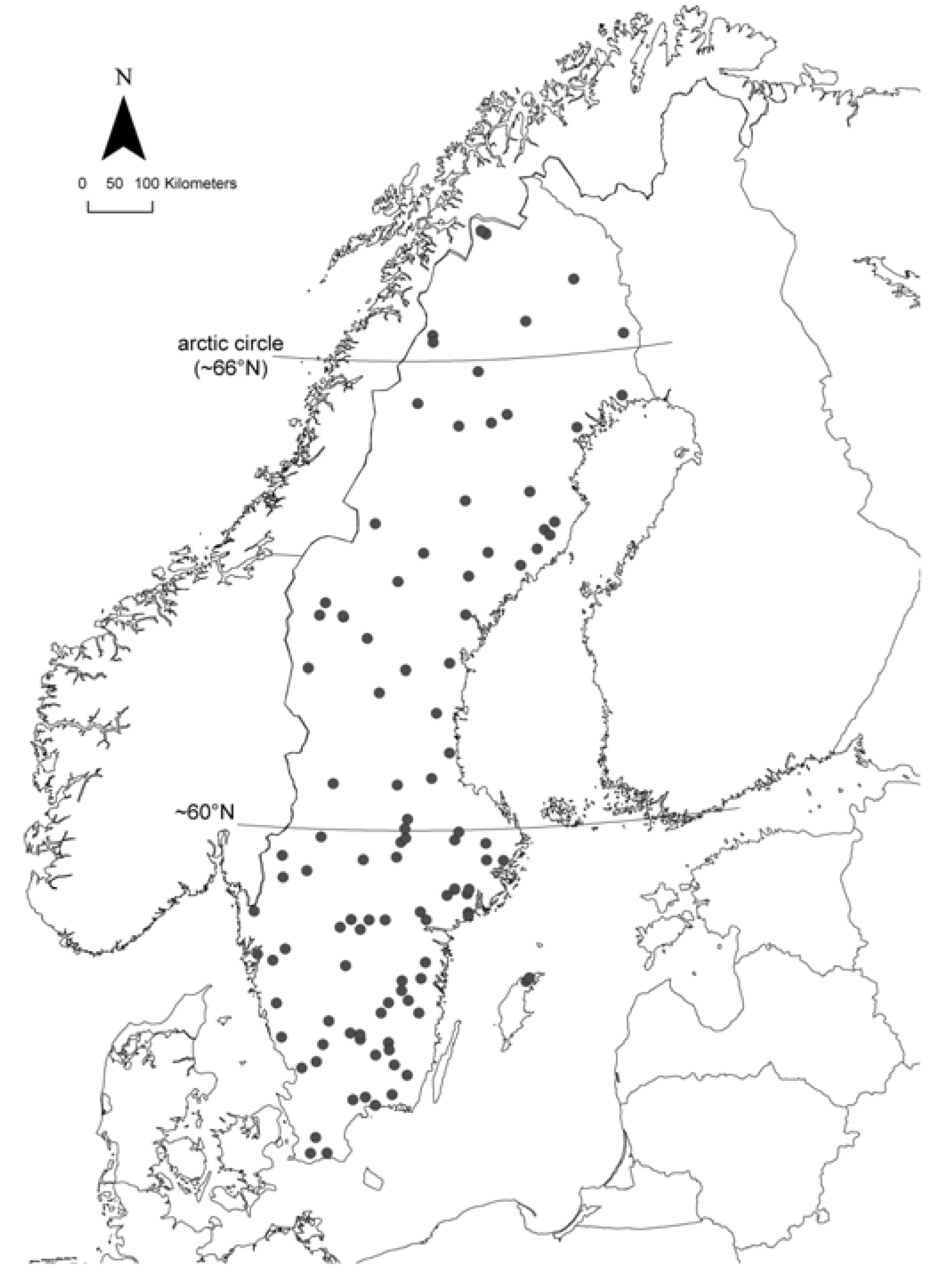
2.1. Study Area and Sampling

Biological and chemical data were acquired from a national environmental monitoring program of regionally representative lake ecosystems [19]. The data set consisted of 105 lakes with biological, chemical and geographical data collected during 2007 and 2008. The study lakes covered broad geographic and climate gradients (Table 1). The lakes were situated in three different ecoregions (sensu Illies, 1978): the Central Plains (n = 56 lakes), the Borealic Uplands (n = 15 lakes) and the Fennoscandian Shield (n = 34 lakes), and covered a south-north gradient in latitude from ~55.5°N to ~68.4°N (Figure 1). Ecosystem size also varied markedly: lake area ranged from 0.02 to 52 km² (mean = 1.9 km²) and catchment area ranged from 0.26 to 2,902 km² (mean = 75 km²). Productivity of the lakes ranged from low, nutrient poor (minimum total nitrogen = 54 µg/L and minimum total phosphorus = 1.75 µg/L) to high, nutrient rich (max total nitrogen = 1,345 µg/L, max total phosphorus = 68 µg/L).

Table 1. Characteristics of the 105 study lakes.

	Median	Mean	Min	Max
altitude (m a.s.l.)	169	250	15	1,138
catchment area (km2)	5.6	75.5	0.26	2,902
lake area (km2)	0.6	1.9	0.02	52.2
lake depth (m)	10	12	1	36
color (filtered absorbance)	0.10	0.14	0.0	0.59
pH	6.67	6.56	5.03	8.27
precipitation per year (mm)	750	752	550	1,150
temperature July (°C)	16	15	8	17
total nitrogen (µg/L)	387	430	54	1,345
total phosphorus (µg/L)	7.6	11.6	1.8	67.6
catchment agriculture (%)	0.0	3.1	0.0	54.4
catchment coniferous forest (%)	3.3	14.2	0.0	75.9
catchment deciduous forest (%)	0.6	2.3	0.0	19.6

Table 1. Characteristics of the 105 study lakes.

	Median	Mean	Min	Max
altitude (m a.s.l.)	169	250	15	1,138
catchment area (km2)	5.6	75.5	0.26	2,902
lake area (km2)	0.6	1.9	0.02	52.2
lake depth (m)	10	12	1	36
color (filtered absorbance)	0.10	0.14	0.0	0.59
pH	6.67	6.56	5.03	8.27
precipitation per year (mm)	750	752	550	1,150
temperature July (°C)	16	15	8	17
total nitrogen (µg/L)	387	430	54	1,345
total phosphorus (µg/L)	7.6	11.6	1.8	67.6
catchment agriculture (%)	0.0	3.1	0.0	54.4
catchment coniferous forest (%)	3.3	14.2	0.0	75.9
catchment deciduous forest (%)	0.6	2.3	0.0	19.6

Figure 1. Map of Sweden showing the location of the lakes used in the study.

Figure 1. Map of Sweden showing the location of the lakes used in the study.

Phytoplankton assemblages were sampled in August of each year by taking a water sample from the epilimnion (0–4 m) using a Plexiglas® tube sampler (diameter = 3 cm). In lakes with a surface area > 1 km², a single mid-lake site was used for sampling. In lakes with a surface area < 1 km², five epilimnetic water samples were pooled to form a composite sample from which a subsample was taken. The samples were preserved with acid Lugol’s iodine solution [20]. Phytoplankton taxa were identified to the lowest taxonomic unit possible (usually species), using an inverted light microscope and the modified Utermöhl technique commonly used in the Nordic countries [21].

Benthic invertebrates were collected from two habitats in late autumn (October–November) each year. Littoral samples were collected using standardized kick sampling [22] with a hand net (0.5 mm mesh size). A composite sample consisting of five standardized kick samples (20 s duration, 0.25 m × 1 m long at about 0.5 m depth, total area 1.25 m²) was taken from hard-bottom, vegetation-free sites in each lake. Profundal samples consisted of five replicate Ekman samples (~247 cm²) taken in the deepest area of the lake. Invertebrate samples were preserved in 70% ethanol until analysis. The samples were processed by sorting with 10 times magnification in the laboratory. Invertebrates were identified and counted using dissecting and light microscopes. Organisms were identified to the lowest taxonomic unit possible, generally to species level.

For both invertebrates and phytoplankton, data for the two years were combined: if a taxon was found in a lake during one of the two years it was considered as present. For some lakes only a single year of data was available (phytoplankton: eleven lakes; littoral benthic invertebrates: six lakes; profundal invertebrates: two lakes). For the models to be able to distinguish between sites with and without a certain species, sufficient information must be available, i.e., there must be enough presences and absences. Therefore, only taxa occurring in more than five lakes and less than 100 lakes were included in the study, resulting in: 129 phytoplankton taxa (215 taxa in total); 164 littoral invertebrate taxa (303 taxa in total) and 44 profundal invertebrate taxa (141 taxa in total).

Water samples were collected from the surface (0.5 m), 2–8 times annually during the two years. Water was collected with a Plexiglas® sampler and kept cool during transport to the laboratory, where the samples were analyzed for pH, nutrient concentrations (total nitrogen and total phosphorus), water color (absorbance of filtered water), and total organic carbon concentration (TOC). All physicochemical analyses were done at the Department of Aquatic Sciences and Assessment, Swedish University of Agricultural Sciences, following international (ISO) or European (EN) standards when available [23]. Geographical information was acquired from digital maps from the National Land Survey of Sweden [24] and climate variables from the Swedish institute for metrology and hydrology [25].

The initial data set of 25 environmental variables was screened for redundancy by pairwise correlations using Spearman’s rank test. Variables were removed until no pair showed a correlation >0.85, leaving a final dataset containing 20 predictor variables (Table 2). Predictor variables were checked for normality using the Shapiro-Wilk’s test [26], and, if necessary, transformed (logarithm) to approximate normality.

Geographical data that describe spatial configuration of the lakes was used to analyze factors influencing model accuracy (Table 3). Distances to neighbor lakes, the number of lakes in vicinity of the study lake, and the amount of water in the catchment were used as proxies for connectivity between lakes. Euclidean distances to the 1st, 5th and 10th neighbor lake and the number of lakes within buffer zones around the lake (100 m, 200 m, 500 m, 1,000 m, 5,000 m and 10,000 m) were calculated using ArcGIS and the amount (area) of water in the catchment, excluding the study lake, was extracted from digital land-use maps.

Table 2. Variables considered for model calibration. Variables in bold were used in model calibration, other removed due to high correlations.

	environmental factor	unit
water chemistry	total phosphorus concentration	µg/L
	total nitrogen concentration	µg/L
	pH
	total organic carbon	mg/L
	calcium concentration	meq/L
	magnesium concentration	meq/L
	potassium concentration	meq/L
	alkalinity	meq/L
catchment land cover	water color1 coniferous forest	km2
	deciduous forest	km2
	mixed forest	km2
	water	km2
	wetland	km2
	agriculture	km2
	pasture	km2
	altitude	m above sea level
geographical	longitude latitude
	catchment area	km2
	lake area	km2
	lake depth	meter
	precipitation2	mm
climate	air temperature July2	Celsius
	length of vegetation period	days

¹ measured as absorbance at 420nm/5cm; ² mean 1961–1990.

Table 2. Variables considered for model calibration. Variables in bold were used in model calibration, other removed due to high correlations.

	environmental factor	unit
water chemistry	total phosphorus concentration	µg/L
	total nitrogen concentration	µg/L
	pH
	total organic carbon	mg/L
	calcium concentration	meq/L
	magnesium concentration	meq/L
	potassium concentration	meq/L
	alkalinity	meq/L
catchment land cover	water color1 coniferous forest	km2
	deciduous forest	km2
	mixed forest	km2
	water	km2
	wetland	km2
	agriculture	km2
	pasture	km2
	altitude	m above sea level
geographical	longitude latitude
	catchment area	km2
	lake area	km2
	lake depth	meter
	precipitation2	mm
climate	air temperature July2	Celsius
	length of vegetation period	days

¹ measured as absorbance at 420nm/5cm; ² mean 1961–1990.

Table 3. Lake characteristics for evaluation of model accuracy.

	source
lake size	Digital maps from the National Land Survey of Sweden [24]
catchment size	Digital maps from the National Land Survey of Sweden [24]
water in catchment-lake area	Corine land cover [28]
altitude	Digital elevation model from the National Land Survey of Sweden [24]
distance to 1st, 5th and 10th lake	Distance to outlet coordinate, using database from Swedish institute for metrology and hydrology [25] containing 105,645 lakes with area ≥ 1 hectare
N lakes within 100, 200, 500, 1,000, 5,000 and 10,000 m buffers	Using database from Swedish institute for metrology and hydrology [25] containing 105,645 lakes with area ≥ 1 hectare

Table 3. Lake characteristics for evaluation of model accuracy.

	source
lake size	Digital maps from the National Land Survey of Sweden [24]
catchment size	Digital maps from the National Land Survey of Sweden [24]
water in catchment-lake area	Corine land cover [28]
altitude	Digital elevation model from the National Land Survey of Sweden [24]
distance to 1st, 5th and 10th lake	Distance to outlet coordinate, using database from Swedish institute for metrology and hydrology [25] containing 105,645 lakes with area ≥ 1 hectare
N lakes within 100, 200, 500, 1,000, 5,000 and 10,000 m buffers	Using database from Swedish institute for metrology and hydrology [25] containing 105,645 lakes with area ≥ 1 hectare

2.2. Modeling

Models were developed using BIOMOD [29], a modeling platform in the R-software [30] which offers several state-of-the-art modeling techniques and ensemble modeling. Six different modeling methods were used: classification tree analysis (CTA), mixture discriminant analysis (MDA), generalized linear models (GLM), multivariate adaptive regression splines (MARS), generalized boosting models (GBM) and random forests (RF). These six modeling methods are commonly used in species distribution modeling studies, and have been shown to perform well [8]. The methods represent three classes of modeling methods, namely classification (CTA and MDA), regression (MARS and GLM), and machine learning (RF, GBM).

In CTA, predictor variables are split using the cut-off value that forms the two most homogenous groups of sites possible (i.e., as many presences or absences as possible). The new groups can then be split again until a group contains only presences or absences or until a pre-set maximum number of splits have been made. Predictions are made by assigning new sites to groups containing only or predominantly absences or presences. MDA is an extension of linear discriminant analysis, which tries to find a linear combination of predictors to discriminate between presences and absences. MARS is a regression method that uses piecewise linear fits which allows the coefficients to vary over predictor variable gradients. GLM is a parametric method that allows a logit link function to describe the relationship between the expected value of the response and the predictors. RF and GBM are both extensions of CTA that combines several “trees” using optimization algorithms. In RF, a random selection of sites and predictors are made for every tree, which reduces problems with predictor variables being correlated. In GBM, observations are weighted for all new trees to improve observations with poor fit in preceding trees.

Because the two organism groups modeled here are taxonomically diverse we did not expect to find one optimal modeling technique for all or even a majority of the taxa, and therefore we used a consensus modeling approach. We used the mean of the occurrence probabilities predicted by the six models as this method has been found to be accurate [11]. The probabilities were converted into presences and absences using the build in function in BIOMOD; this was done for each species using the threshold which resulted in the minimum absolute difference between sensitivity and specificity [31].

The models were calibrated and validated using five-fold cross-validation. The dataset was randomly divided into five equally sized parts, stratified by the three ecoregions (Central Plains, Fennoscandian Shield and Borealic Uplands [32]). Models were calibrated on 80% of the sites, and the remaining 20% were used for validation. Calibration was repeated five times so that predictions independent from the calibration procedure were acquired for all 105 lakes.

Because some of the predictor variables are related to dispersal (e.g., lake surface area), the models were also calibrated using the entire dataset to estimate the importance of the predictor variables. BIOMOD does this by applying the model to the data, permuting one of the variables and re-applying the model, and then calculating the correlation between the two sets of predictions. If the predictions with the permuted variables are similar to the ones made with the real variable (i.e., high correlation), the variable is probably not important for the species distribution. The correlation could be negative, indicating an even greater influence of the permutated variable on the prediction than with a correlation of 0. The variable importance is expressed as 1-correlation, i.e., important variables have high values.

2.3. Evaluation of Model Accuracy

The cross-validation predictions for the individual models and the consensus model were used to calculate AUC, a measure of model performance commonly used in SDM studies. AUC, the area under the receiver operator curve, was calculated for all taxa by plotting sensitivity (the ability for model to predict presences) versus 1-specificity (the ability for model to predict absences) for all possible threshold values used to convert probability predictions to presence-absence predictions, i.e., all predicted probabilities for a species to occur at individual sites. The AUC measure is therefore independent of species prevalence, in contrast to other measures, such as the proportion of observations correctly predicted. AUC was calculated using the verification package [33] in R-software. AUC ranges from 0 to 1, with 1 indicating a perfect model, and values < 0.5 indicate a model no better or worse than random. We also calculated the proportion of species found that were predicted to be present, i.e., the true positive rate (TPR), also referred to as accuracy of assemblage prediction.

2.3.1. Invertebrate Flight Ability

Invertebrate taxa were divided into three classes according to their flight ability (no, low, or high). Odonata were the largest (flying) organisms in the dataset and were classified as having a high flight ability, whereas insect orders, such as Trichoptera and Diptera, were classified as having a low flight ability, and wingless invertebrates, such as Gastropoda and Nematoda, were classified as having no flight ability. T-tests were used to test differences in AUC between the three groups. Taxa recorded from both littoral and profundal habitats were modeled twice, and the highest AUC was used.

2.3.2. Ecosystem Connectivity

To determine how landscape configuration and flight ability (for invertebrates) influence model accuracy, correlations between true positive rate (TPR) and indicators for connectivity (altitude, distance to neighbor lakes, other lakes/streams in catchment, lakes within a buffer zone of 100 m, 200 m, 500 m, 1,000 m, 5,000 m and 10,000 m from the shoreline) and lake size were analyzed with Spearman rank correlation, using computer software JMP [34].

3. Results

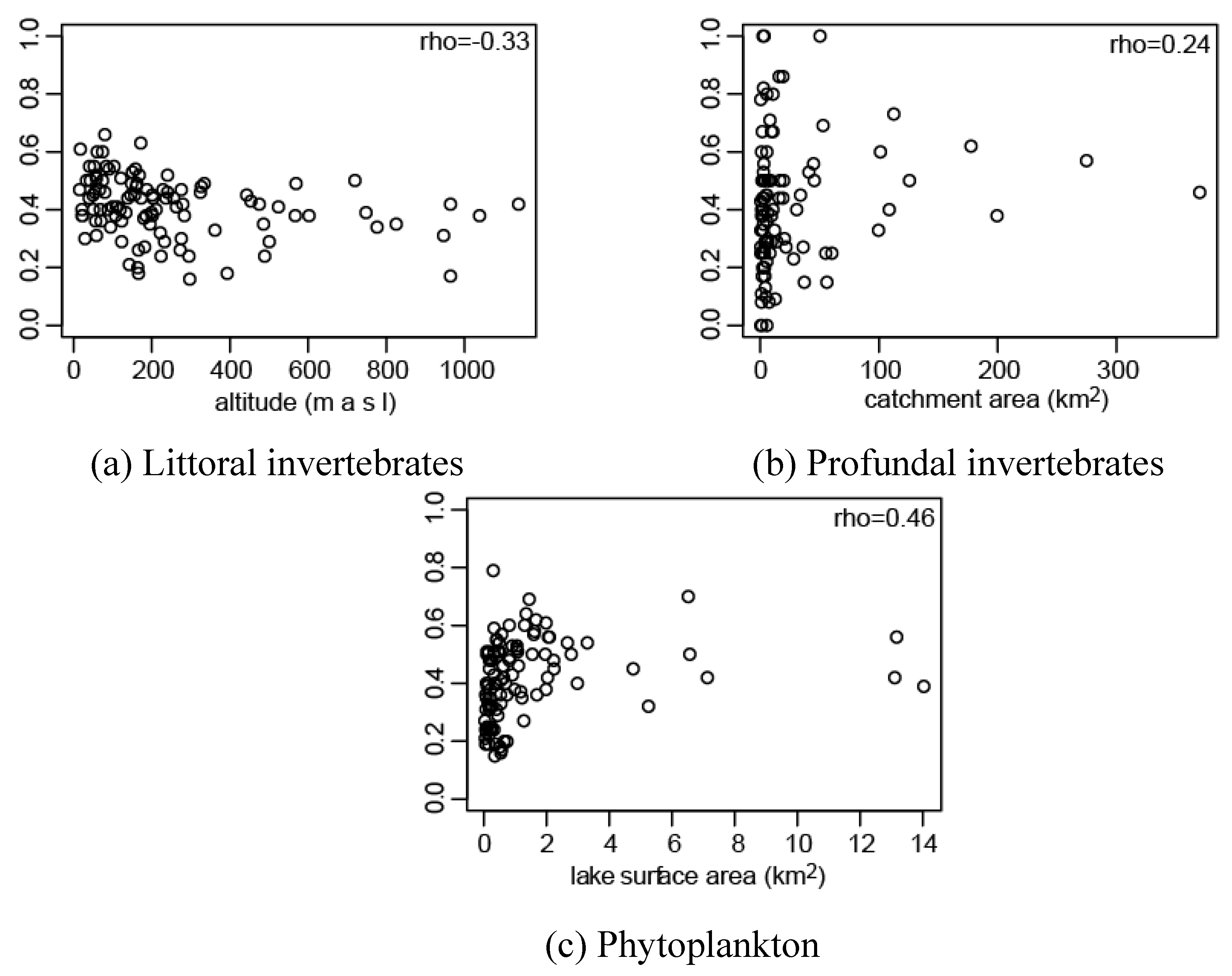
3.1. Effect of Connectivity and Ecosystem Size on Assemblage Prediction Accuracy

For 99% of the lakes, at least one other lake was situated within a 5,000 m radius, and for 70% of the lakes at least 10 other lakes were situated within a 5,000 m radius. Distance to the closest neighbor lake ranged from 186 to 9,905 m, with a mean distance of 1,360 m. For only one of the study lakes the distance was more than 5,000 m. The distance to the 10th closest neighbor lake ranged from 4,669 m to 18,805 m.

Model accuracy was low for lakes presumed to be more isolated, e.g., the accuracy of assemblage prediction (TPR) was significantly and negatively correlated with altitude for littoral invertebrates (Figure 2 and Table 4). Moreover, predictions of profundal assemblages were more accurate for lakes situated in larger catchments, whereas the accuracy of predictions of phytoplankton assemblage composition was positively correlated to lake and catchment size, and the amount of water in the catchment. By contrast, both littoral invertebrate and phytoplankton assemblages were more accurately predicted when distances to other lakes were greater, and littoral assemblages were more accurately predicted when fewer lakes were present in the 10,000 m buffer zone. Lake Ymsen in central Sweden had almost 10,000 m to the closest neighbor lake, which is more than twice as far as the one with 2nd longest distance; however, removing Lake Ymsen from the correlation analysis did not change the outcome of the tests.

Table 4. Correlations between true positive rate of model predictions and landscape configuration indices. Spearman correlations between the proportion of species found at a lake correctly predicted as present (true positive rate) and indicators of ecosystem size and spatial configuration. Distance neighbor is the distance to the closest and 2nd, 5th and 10th closest neighbor lake and N lakes is the number of lakes with 100, 200, 500, 1,000 and 5,000 m buffer zones round the lake shoreline. Significant (p ≤ 0.05) correlations in bold. Asterisks indicate significance level: * p ≤ 0.05, ** p ≤ 0.01, *** p ≤ 0.001.

	littoral	profundal	phytoplankton
lake area	0.07	0.18	0.46***
catchment area	0.03	0.24*	0.43***
water (excl. study lake)	0.07	0.03	0.37***
altitude	−0.33***	0.00	−0.07
distance neighbor 1	0.13	−0.02	0.18
distance neighbor 2	0.12	0.04	0.23*
distance neighbor 5	0.15	0.08	0.30**
distance neighbor 10	0.19*	0.11	0.22*
N lakes 100 m	0.00	0.04	0.03
N lakes 200 m	0.08	0.14	0.07
N lakes 500 m	0.00	0.03	0.13
N lakes 1,000 m	−0.05	−0.07	0.08
N lakes 5,000 m	−0.17	−0.06	−0.07
N lakes 10,000 m	−0.22*	−0.01	−0.02

Table 4. Correlations between true positive rate of model predictions and landscape configuration indices. Spearman correlations between the proportion of species found at a lake correctly predicted as present (true positive rate) and indicators of ecosystem size and spatial configuration. Distance neighbor is the distance to the closest and 2nd, 5th and 10th closest neighbor lake and N lakes is the number of lakes with 100, 200, 500, 1,000 and 5,000 m buffer zones round the lake shoreline. Significant (p ≤ 0.05) correlations in bold. Asterisks indicate significance level: * p ≤ 0.05, ** p ≤ 0.01, *** p ≤ 0.001.

	littoral	profundal	phytoplankton
lake area	0.07	0.18	0.46***
catchment area	0.03	0.24*	0.43***
water (excl. study lake)	0.07	0.03	0.37***
altitude	−0.33***	0.00	−0.07
distance neighbor 1	0.13	−0.02	0.18
distance neighbor 2	0.12	0.04	0.23*
distance neighbor 5	0.15	0.08	0.30**
distance neighbor 10	0.19*	0.11	0.22*
N lakes 100 m	0.00	0.04	0.03
N lakes 200 m	0.08	0.14	0.07
N lakes 500 m	0.00	0.03	0.13
N lakes 1,000 m	−0.05	−0.07	0.08
N lakes 5,000 m	−0.17	−0.06	−0.07
N lakes 10,000 m	−0.22*	−0.01	−0.02

Figure 2. Examples of the significant correlations (Spearman correlation) between model accuracy expressed as true positive rate and geographical properties of study lakes: (a) littoral invertebrates and altitude, (b) profundal invertebrates and catchment area (two lakes with catchment area > 2000 km² excluded did not affect the correlation analysis) and (c) phytoplankton and lake area (one lake with surface area of 52 km² excluded did not affect the correlation analysis).

Figure 2. Examples of the significant correlations (Spearman correlation) between model accuracy expressed as true positive rate and geographical properties of study lakes: (a) littoral invertebrates and altitude, (b) profundal invertebrates and catchment area (two lakes with catchment area > 2000 km² excluded did not affect the correlation analysis) and (c) phytoplankton and lake area (one lake with surface area of 52 km² excluded did not affect the correlation analysis).

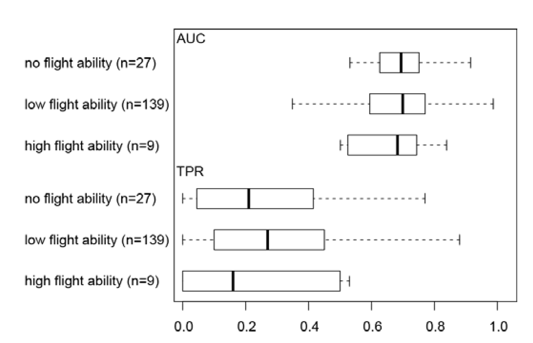
3.2. Effect of Flight Ability on Invertebrate Distribution Prediction Accuracy

Our study gave no support to the conjecture that species distribution model accuracy varies with the dispersal ability. AUC values ranged from 0.66 to 0.70 (no flight ability: mean = 0.70 ± 0.12; n = 27; low flight ability: mean = 0.68 ± 0.15; n = 139; high flight ability: mean = 0.66 ± 0.12; n = 9; Figure 3) and true positive rate ranged from 0 to 0.88 (no flight ability: mean = 0.27 ± 0.26; n = 27; low flight ability: mean = 0.28 ± 0.22; n = 139; high flight ability: mean=0.25 ± 0.25; n = 9; Figure 3). No significant differences in mean AUC or true positive rate were found for the three groups of invertebrates with varying flight ability. For example, the distribution of the chironomid midge Synorthocladius semivirens, which was classified as having low flight ability, and odonate Aeshna grandis, which was classified as having high flight ability, were poorly predicted (AUC was 0.23 and 0.52, respectively). By contrast, the distribution of gastropod Bithynia tentaculata was accurately predicted (AUC was 0.91).

Figure 3. Boxplot of model accuracy (AUC and TPR) per taxon grouped according to their flight ability. No significant differences in mean values between the groups were found (t-test; p > 0.05).

Figure 3. Boxplot of model accuracy (AUC and TPR) per taxon grouped according to their flight ability. No significant differences in mean values between the groups were found (t-test; p > 0.05).

3.3. Importance of Predictor Variables

The importance of predictor variables for model accuracy varied widely across taxa and with modeling method (Table 5). However, some general trends were observed. Phosphorus and pH were better predictors of phytoplankton than of invertebrate taxa. TOC was important for all habitat/taxa groups of organisms. Water color (abs-f) was a better predictor of profundal invertebrates and phytoplankton than for littoral invertebrates. By contrast, altitude and lake area were better predictors of littoral invertebrates, and depth was the most important predictor of profundal invertebrate assemblages.

Table 5. Variable importance: 75th percentile (Q75) and maximum predictor variable influence (variable importance) for the prediction of littoral and profundal invertebrates and phytoplankton distribution. N per variable = number of species × 6 modeling techniques, i.e., littoral = 984, profundal = 264, phytoplankton = 774. The distribution of variable importance is skewed towards zero, and therefore the 75th percentile (Q75) and maximum are reported.

		littoral		profundal		phytoplankton
	environmental variables	Q75	max	Q75	max	Q75	max
water chemistry	total phosphorus concentration	0.05	1.58	0.10	1.09	0.27	1.07
	total nitrogen concentration	0.01	1.11	0.02	1.13	0.04	1.33
	pH	0.06	1.20	0.06	1.15	0.25	1.34
	TOC	0.36	1.62	0.36	1.21	0.32	1.42
	calcium concentration	0.02	1.15	0.03	1.09	0.04	1.13
	magnesium concentration	0.01	1.50	0.00	1.08	0.03	1.46
	potassium concentration	0.01	1.19	0.01	1.24	0.01	1.14
	water color	0.03	1.42	0.10	1.04	0.10	1.11
land use	coniferous forest	0.01	1.09	0.04	1.09	0.01	1.01
	deciduous forest	0.01	1.09	0.01	0.93	0.00	1.01
	mixed forest	0.01	0.97	0.01	0.78	0.00	1.39
	wetland	0.01	1.16	0.00	0.95	0.00	0.90
	agriculture	0.00	1.15	0.00	0.74	0.00	1.13
	pasture	0.00	1.04	0.00	1.10	0.00	1.04
geographical	altitude	0.20	1.21	0.06	1.05	0.04	1.18
	catchment area	0.01	1.12	0.06	1.23	0.01	1.14
	lake area	0.12	1.13	0.01	1.07	0.01	1.73
	lake depth	0.01	1.22	0.45	1.14	0.01	1.14
climate	precipitation	0.00	0.93	0.00	0.75	0.00	1.08
	length of vegetation period	0.00	1.20	0.00	1.09	0.00	1.00

Table 5. Variable importance: 75th percentile (Q75) and maximum predictor variable influence (variable importance) for the prediction of littoral and profundal invertebrates and phytoplankton distribution. N per variable = number of species × 6 modeling techniques, i.e., littoral = 984, profundal = 264, phytoplankton = 774. The distribution of variable importance is skewed towards zero, and therefore the 75th percentile (Q75) and maximum are reported.

		littoral		profundal		phytoplankton
	environmental variables	Q75	max	Q75	max	Q75	max
water chemistry	total phosphorus concentration	0.05	1.58	0.10	1.09	0.27	1.07
	total nitrogen concentration	0.01	1.11	0.02	1.13	0.04	1.33
	pH	0.06	1.20	0.06	1.15	0.25	1.34
	TOC	0.36	1.62	0.36	1.21	0.32	1.42
	calcium concentration	0.02	1.15	0.03	1.09	0.04	1.13
	magnesium concentration	0.01	1.50	0.00	1.08	0.03	1.46
	potassium concentration	0.01	1.19	0.01	1.24	0.01	1.14
	water color	0.03	1.42	0.10	1.04	0.10	1.11
land use	coniferous forest	0.01	1.09	0.04	1.09	0.01	1.01
	deciduous forest	0.01	1.09	0.01	0.93	0.00	1.01
	mixed forest	0.01	0.97	0.01	0.78	0.00	1.39
	wetland	0.01	1.16	0.00	0.95	0.00	0.90
	agriculture	0.00	1.15	0.00	0.74	0.00	1.13
	pasture	0.00	1.04	0.00	1.10	0.00	1.04
geographical	altitude	0.20	1.21	0.06	1.05	0.04	1.18
	catchment area	0.01	1.12	0.06	1.23	0.01	1.14
	lake area	0.12	1.13	0.01	1.07	0.01	1.73
	lake depth	0.01	1.22	0.45	1.14	0.01	1.14
climate	precipitation	0.00	0.93	0.00	0.75	0.00	1.08
	length of vegetation period	0.00	1.20	0.00	1.09	0.00	1.00

4. Discussion

Failure to incorporate species dispersal ability and ecosystem connectivity and size into SDMs could limit their usefulness for ecological applications. In this study, we studied if variations in model performance among species and among ecosystems can be explained by the species’ dispersal ability and the landscape configuration of the ecosystems. AUC and TPR, the indices of model accuracy used here, can also been seen as the correlation between measured environmental variables and species distribution or assemblage composition. If a species distribution or assemble composition is highly correlated with the environment, then species distribution or assemble composition mainly depends on the environment. If, on the other hand, the correlation is low, other factors, such as biological interactions, dispersal limitations, or disturbances, are probably more important.

4.1. Effect of Connectivity and Ecosystem Size on Assemblage Prediction Accuracy

The accuracy of predictions of littoral and profundal invertebrate and phytoplankton assemblages were positively affected by size of the ecosystem, whilst littoral assemblage predictions were less accurate for lakes at higher altitudes, supporting our hypothesis that model accuracy is higher for ecosystems which are easier to colonize. Conversely, littoral invertebrates were not affected by ecosystem size, and both predictions of littoral invertebrate assemblages and phytoplankton assemblages were more accurate in isolated lakes (high distance to neighboring lakes). Furthermore, littoral assemblages were less accurate when the number of lakes within a 10,000 m buffer zone was high. The finding that littoral invertebrates were found to be less affected by ecosystem size than phytoplankton or profundal invertebrates could be due to that organisms inhabiting the littoral zone generally are better flyers and less dependent on passive (air) dispersal. For example, profundal habitats are often composed of taxa with relatively weak (chironomid midges) or no flight ability (oligochates), whereas littoral habitats are often composed of larger insects with stronger flight ability, such as mayflies, caddisflies and odonates.

The use of true positive rate requires the probabilities from the model to be converted to presence–absence, and the method used affects a model’s sensitivity and specificity (ability to correctly predicted present and absent species, respectively) [31]. For example, a high threshold will favor sensitivity, which will result in a high true positive rate, but the overall predictive power of the model will be poor. We used a method that rates false positive and false negative errors equally, and could therefore use true positive rate as an index of model performance.

Our finding that littoral and phytoplankton assemblages were more accurately predicted in lakes with greater distance to neighboring lakes could be related to dispersal from nearby lakes resulting homogenization of assemblage composition, whereas lake-specific factors, such has differences in habitat (e.g., substratum composition for littoral invertebrate assemblages and nutrients or humic content for phytoplankton assemblages), become more important as distance between lakes increases.

4.2. Effect of Flight Ability on Invertebrate Distribution Prediction Accuracy

No support for dispersal limitation was found when model accuracy was compared among groups of invertebrates with varying flight ability. Indeed, taxa with no flight ability were predicted as well as taxa classified as having low or high flight ability, which contrasts with our finding that altitude affected model accuracy for littoral invertebrates. This discrepancy could be due to either our classification of flight ability not reflecting dispersal at larger scale, or altitude affecting model performance in a way not related to dispersal. Information on the dispersal ability of aquatic species is scarce, although a few studies have attempted to quantify the dispersal range of some large insect species, such as mayflies [35]. Our division of flight ability into three classes was relatively simplistic, and better estimates, for example from trap studies, could reveal stronger effects of dispersal ability. Furthermore, not only adult insects are dispersed by air and wind, but also eggs and organisms with cryptoniotic life stages can be dispersed by wind, and the size of the wind-dispersed propagules can affect dispersal distance [36]. However, support for our conjecture that organisms with poor flight ability are less able to disperse is given by Kovats et al. [35], who found that smaller caddisflies are less able to disperse than larger caddisflies and mayflies (Hexagenia). Kovats et al. [35] also found that inland dispersal of mayflies and caddisflies was low, although they found individuals in light traps five kilometers from shore. Almost all of the lakes in our study had another lake within a five-kilometer radius, and it is therefore likely that most if not all taxa have the possibility to migrate between sites.

The models in our study also included factors related to dispersal and colonization, such as lake surface area, catchment area and altitude, and therefore dispersal-limited species could be predicted as being absent from lakes that are more difficult to colonize (e.g., lakes with a small surface area). Similar to our study, Hanspach et al. [37] found no effect of dispersal type (wind, self, water and animal dispersal) on the performance of models predicting the distribution of vascular plants. Poyry et al. [38], on the other hand, found that model accuracy was low for butterflies with high mobility and longer flight periods, but also that model accuracy was high for species with large body size, which, according to the authors, could be because of a higher probability of detection, or higher mobility (i.e., dispersal ability).

5. Conclusions

The results from this study suggest that there are effects of species dispersal ability on model performance for boreal lake ecosystems. Landscape configuration was found to be important for model predictions, particularly for phytoplankton (ecosystem size and connectivity) but also for littoral (connectivity) and profundal (ecosystem size) assemblages. This finding could have implications for the application of species distribution models in environmental assessment as well as management of ecosystem biodiversity. However, the extent of the consequences for applications needs to be assessed further.

Our finding that dispersal traits had little effect on model accuracy, could be due to the following: (i) most taxa are not dispersal-limited; (ii) dispersal and colonization constraints are directly or indirectly incorporated in the models; or (iii) our wing size classifications were overly simplistic. As discussed above, the dispersal ability of most invertebrates is not well known, although some studies suggest that distances of less than five kilometers do not hamper colonization across land barriers. Dispersal ability is, however, only one of several factors that can affect model accuracy; hence distinguishing a “dispersal signal” is difficult. Although we did not measure dispersal per se, our finding that spatial configuration was important for model performance likely reflects dispersal and colonization processes. Therefore, we suggest that factors related to dispersal and connectivity should be included in SDMs as predictors. The importance of dispersal on model performance should be tested further using other organism groups and study areas, and other methods, such as experiments and genetics [39].

References and Notes

1. Moore, K.A.; Elmendorf, S.C. Propagule vs. niche limitation: untangling the mechanisms behind plant speciesʼ distributions. Ecol. Lett. 2006, 9, 797–804. [Google Scholar] [CrossRef]
2. Thuiller, W.; Lavorel, S.; Araujo, M.B.; Sykes, M.T.; Prentice, I.C. Climate change threats to plant diversity in Europe. Proc. Natl. Acad. Sci. USA 2005, 102, 8245–8250. [Google Scholar] [CrossRef]
3. Thomas, C.D.; Cameron, A.; Green, R.E.; Bakkenes, M.; Beaumont, L.J.; Collingham, Y.C.; Erasmus, B.F.N.; de Siqueira, M.F.; Grainger, A.; Hannah, L.; et al. Extinction risk from climate change. Nature 2004, 427, 145–148. [Google Scholar] [CrossRef] [Green Version]
4. Peterson, A.T.; Vieglais, D.A. Predicting species invasions using ecological niche modeling: new approaches from bioinformatics attack a pressing problem. Bioscience 2001, 51, 363–371. [Google Scholar] [CrossRef]
5. Hawkins, C.P.; Norris, R.H.; Hogue, J.N.; Feminella, J.W. Development and evaluation of predictive models for measuring the biological integrity of streams. Ecol. Appl. 2000, 10, 1456–1477. [Google Scholar] [CrossRef]
6. Hutchinson, G.E. Concluding remarks Cold Spring Harbor Symp. Quantitative Biol. 1957, 22, 415–427. [Google Scholar] [CrossRef]
7. Leibold, M.A.; Holyoak, M.; Mouquet, N.; Amarasekare, P.; Chase, J.M.; Hoopes, M.F.; Holt, R.D.; Shurin, J.B.; Law, R.; Tilman, D.; et al. The metacommunity concept: a framework for multi-scale community ecology. Ecol. Lett. 2004, 7, 601–613. [Google Scholar] [CrossRef]
8. Elith, J.; Graham, C.H.; Anderson, R.P.; Dudik, M.; Ferrier, S.; Guisan, A.; Hijmans, R.J.; Huettmann, F.; Leathwick, J.R.; Lehmann, A.; Li, J.; et al. Novel methods improve prediction of speciesʼ distributions from occurrence data. Ecography 2006, 29, 129–151. [Google Scholar] [CrossRef]
9. Guisan, A.; Zimmermann, N.E.; Elith, J.; Graham, C.H.; Phillips, S.; Peterson, A.T. What matters for predicting the occurrences of trees: Techniques, data, or speciesʼ characteristics? Eco. Monogr. 2007, 77, 615–630. [Google Scholar] [CrossRef]
10. Thuiller, W. BIOMOD-optimizing predictions of species distributions and projecting potential future shifts under global change. Global Change Biol. 2003, 9, 1353–1362. [Google Scholar] [CrossRef]
11. Marmion, M.; Parviainen, M.; Luoto, M.; Heikkinen, R.K.; Thuiller, W. Evaluation of consensus methods in predictive species distribution modelling. Divers. Distrib. 2009, 15, 59–69. [Google Scholar] [CrossRef]
12. Kadmon, R.; Farber, O.; Danin, A. A systematic analysis of factors affecting the performance of climatic envelope models. Ecol. Appl. 2003, 13, 853–867. [Google Scholar] [CrossRef]
13. Newbold, T.; Reader, T.; Zalat, S.; El-Gabbas, A.; Gilbert, F. Effect of characteristics of butterfly species on the accuracy of distribution models in an arid environment. Biodiver. Conserv. 2009, 18, 3629–3641. [Google Scholar] [CrossRef]
14. Göthe, E.; Angeler, D.G.; Sandin, L. Metacommunity structure in a small boreal stream network. J. Anim. Ecol. 2013, 82, 449–458. [Google Scholar] [CrossRef]
15. MacArthur, R.H.; Wilson, E.O. The Theory of Island Biogeography; Princeton University Press: Princeton, NJ, USA, 1967. [Google Scholar]
16. Allouche, O.; Steinitz, O.; Rotem, D.; Rosenfeld, A.; Kadmon, R. Incorporating distance constraints into species distribution models. J. Appl. Ecol. 2008, 45, 599–609. [Google Scholar] [CrossRef]
17. Vaughan, I.P.; Ormerod, S.J. The continuing challenges of testing species distribution models. J. Appl. Ecol. 2005, 42, 720–730. [Google Scholar] [CrossRef]
18. Vaughan, I.P.; Ormerod, S.J. Increasing the value of principal components analysis for simplifying ecological data: a case study with rivers and river birds. J. Appl. Ecol. 2005, 42, 487–497. [Google Scholar] [CrossRef]
19. Johnson, R.K. Regional Representativeness of Swedish Reference Lakes. Environ. Manage. 1999, 23, 115–124. [Google Scholar] [CrossRef]
20. Throndsen, J. Preservation and storage. In Phytoplankton Manual Monographs on Oceanographic Methodology; Sournia, A., Ed.; UNESCO: Paris, France, 1978; pp. 70–71. [Google Scholar]
21. Olrik, K.P.; Blomqvist, P.; Brettum, P.; Cronberg, G.; Eloranta, P. Methods for Quantitative Assessment of Phytoplankton in Freshwaters, Part I; Report 4860; Swedish Environmental Protection Agency: Stockholm, Sweden, 1989.
22. European Committee for Standardization, Water Quality-Methods for Biological Sampling-Guidance on Handnet Sampling of Aquatic Benthic Macro-Invertebrates; CEN: Brussels, Belgium, 1994.
23. Wilander, A.; Johnson, R.K.; Goedkoop, W. Riksinventering 2000: En synoptisk studie av vattenkemi och bottenfauna i svenska sjöar och vattendrag (in Swedish); Department of Environmental Assessment: Uppsala, Sweden, 2003.
24. National land survey of Sweden. Available online: www.lantmateriet.se/ (accessed on 1 April 2013).
25. Swedish institute for metrology and hydrology. Available online: www.smhi.se/ (accessed on 1 April 2013).
26. Shapiro, S.S.; Wilk, M.B. An analysis of variance test for normality (complete samples). Biometrika 1965, 52, 591–611. [Google Scholar]
27. ESRI homepage. Available online: http://www.esri.com/ (accessed on 1 April 2013).
28. Heymann, Y.; Steenmans, C.; Croissille, G.; Bossard, M. Corine Land Cover; Technical Guide; Office for Official Publications of the European Communities: Luxembourg, Luxembourg, 1994. [Google Scholar]
29. Thuiller, W.; Lafourcade, B.; Engler, R.; Araújo, M.B. BIOMOD-a platform for ensemble forecasting of species distributions. Ecography 2009, 32, 369–373. [Google Scholar] [CrossRef]
30. R Development Core Team, R: A Language and Environment for Statistical Computing; R Foundation for Statistical Computing: Vienna, Austria, 2007.
31. Jiménez-Valverde, A.; Lobo, J.M. Threshold criteria for conversion of probability of species presence to either–or presence–absence. Acta Oecol. 2007, 31, 361–369. [Google Scholar] [CrossRef]
32. Illies, J. Limnofauna Europaea; Gustav Fisher Verlag: Stuttgart, Germany, 1978. [Google Scholar]
33. NCAR-Research Application Program. Verification: Forecast verification utilities. Available online: http://CRAN.R-project.org/package=verification/ (accessed on 1 April 2013).
34. JMP homepage. Available online: http://www.jmp.com/ (accessed on 1 April 2013).
35. Kovats, Z.E.; Ciborowski, J.J.H.; Corkum, L.D. Inland dispersal of adult aquatic insects. Freshwater Biol. 1996, 36, 265–276. [Google Scholar] [CrossRef]
36. Vanschoenwinkel, B.; Gielen, S.; Seaman, M.; Brendonck, L. Wind mediated dispersal of freshwater invertebrates in a rock pool metacommunity: differences in dispersal capacities and modes. Hydrobiologia 2009, 635, 363–372. [Google Scholar] [CrossRef]
37. Hanspach, J.; Kuhn, I.; Pompe, S.; Klotz, S. Predictive performance of plant species distribution models depends on species traits. Perspect Plant Ecol. 2010, 12, 219–225. [Google Scholar] [CrossRef]
38. Poyry, J.; Luoto, M.; Heikkinen, R.K.; Saarinen, K. Species traits are associated with the quality of bioclimatic models. Global Ecol. Biogeogr. 2008, 17, 403–414. [Google Scholar] [CrossRef]
39. Raybould, A.F.; Clarke, R.T.; Bond, J.M.; Welters, R.E.; Gliddon, C.J. Inferring patterns of dispersal from allele frequency data. In Dispersal ecology; Bullock, J.M., Kenward, R.E., Hails, R.S., Eds.; Blackwell Science: Oxford, UK, 2002; pp. 89–110. [Google Scholar]