Relaxation Time and the Problem of the Pleistocene

Department of Geology, University of Georgia, Athens, GA 30602-2501, USA
Diversity 2013, 5(2), 276-292; https://doi.org/10.3390/d5020276
Submission received: 25 February 2013
/
Revised: 4 April 2013
/
Accepted: 9 April 2013
/
Published: 15 April 2013
(This article belongs to the Special Issue Marine Biodiversity)
Abstract
:Although changes in habitat area, driven by changes in sea level, have long been considered as a possible cause of marine diversity change in the Phanerozoic, the lack of Pleistocene extinction in the Californian Province has raised doubts, given the large and rapid sea-level changes during the Pleistocene. Neutral models of metacommunities presented here suggest that diversity responds rapidly to changes in habitat area, with relaxation times of a few hundred to a few thousand years. Relaxation time is controlled partly by metacommunity size, implying that different provinces or trophic levels might have measurably different responses to changes in habitable area. Geologically short relaxation times imply that metacommunities should be able to stay nearly in equilibrium with all but the most rapid changes in area. A simulation of the Californian Province during the Pleistocene confirms this, with the longest lags in diversity approaching 20 kyr. The apparent lack of Pleistocene extinction in the Californian Province likely results from the difficulty of sampling rare species, coupled with repopulation from adjacent deep-water or warm-water regions.
1. Introduction
Because sea level strongly affects the area of shallow-marine habitats [1,2,3,4,5,6], paleobiologists have long argued that sea level should be an important control on the diversity of shallow-marine communities [7,8,9,10,11,12,13,14,15]. Despite abundant anecdotal evidence supporting this relationship [14,15], numerous studies have cast doubt on the effect of sea level on shallow-marine diversity [16,17,18,19,20,21], although some have recognized its role [22]. One of the most compelling counterarguments to the importance of sea level and changes in habitat area has been the lack of elevated marine extinction during the repeated and large changes of sea level during the Pleistocene (2.59 Ma–11.7 ka) [18]. Sea level oscillated widely during the Pleistocene, with up to 110 m change in as little as 15 kyr; changes extreme enough to expose the modern continental shelf [23,24,25]. The problem of the Pleistocene is the lack of marine extinction given what should have been extreme changes in habitat area.
A common hypothesis for the lack of Pleistocene marine extinction is that the changes in area were too rapid and too short-lived for communities to respond [14,18]. Relaxation time is the time it takes for a biota to adjust to a diversity level appropriate for the available area [18,26], and it is essentially unknown for marine systems. A related concept is extinction debt, which refers to the extinction that has yet to take place before a new, lower equilibrium diversity is reached following habitat loss [27].
Measuring relaxation time in the fossil record would be difficult for two reasons. First, the inaccessibility of strata in the subsurface and the erosion of strata that have been exposed hinder accurate measurement of habitat area, and these factors complicate the measurement of diversity as well [28]. Second, cycles in sea level occur over periods ranging from tens of thousands of years to hundreds of millions of years, causing sea level to be in a nearly continuous flux [24], making it difficult to isolate the relaxation time from any particular sea-level change.
Given the difficulties of directly measuring relaxation time in the fossil record, the aim of this study is to use numerical simulations to estimate relaxation time. These estimates will be used to understand the lack of Pleistocene extinction in particular and the relationship of sea-level change, habitat area, and diversity more generally through the Phanerozoic.
2. Numerical Simulations
The numerical simulations used here depict a neutral metacommunity, similar to those used in the Unified Neutral Theory of Biodiversity and Biogeography [29]. The model depicts the birth and death of individuals of species over a very large area, such as a province, and making individuals of all species identical in their probabilities of birth and death produces neutrality. There is no spatial structure to the metacommunity, and the metacommunity is well mixed, such that species may disperse anywhere equally. The metacommunity depicts a single trophic level, such as first-order consumers. For a given area, there are a fixed number of habitable sites, each of which is occupied by a single individual, making the model follow zero-sum dynamics. All simulations were performed in R [30] and the source code is available upon request. Parameters for all models are listed in Table 1.
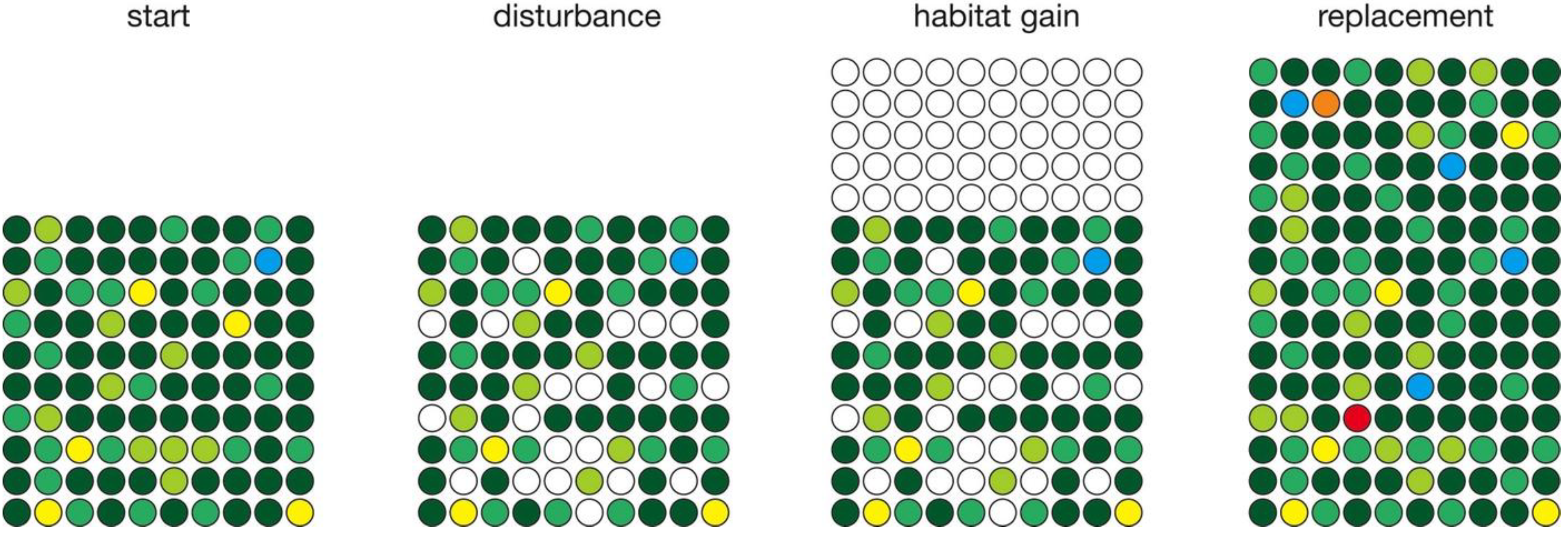
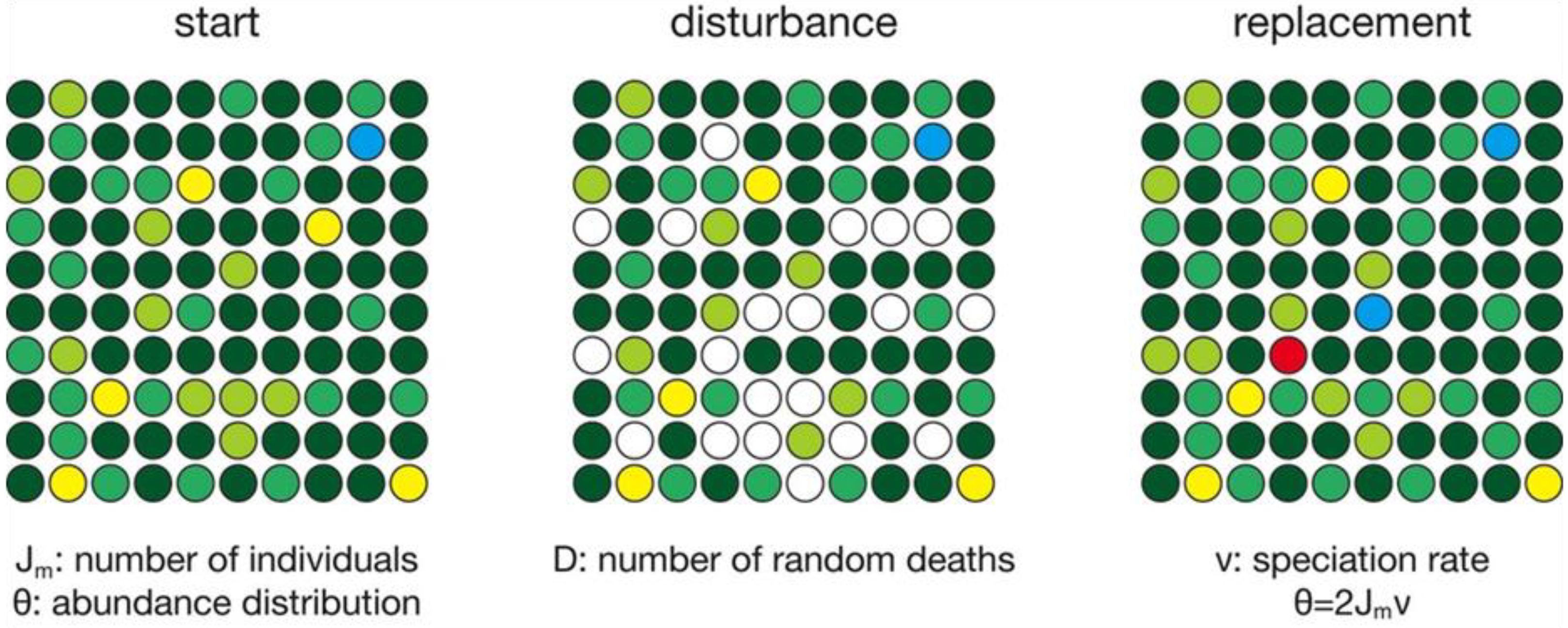
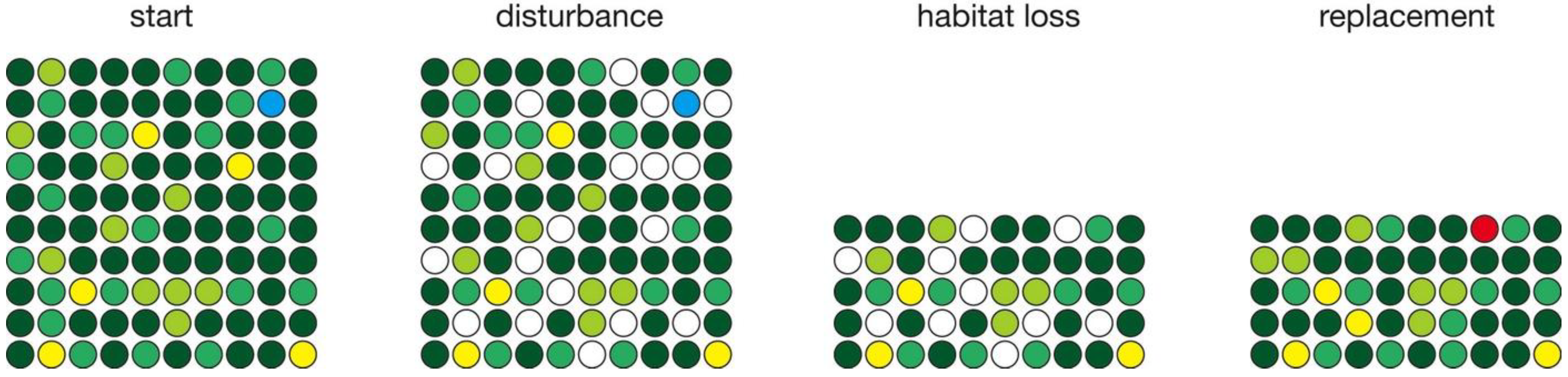
A scaled-down schematic illustrates the model steps (Figure 1). In this example, there are 100 habitable sites, each of which is occupied by an individual of a given species, shown by different colors. The total number of sites therefore equals the total number of individuals in the metacommunity (Jm). The starting abundance distribution of individuals within species is based on Jm and a specified value of Hubbell’s θ [29], and it is calculated with the rand. neutral() function in the untb package of R [31]. Hubbell’s θ is defined as θ = 2Jmν, where ν is the per-individual probability of speciation, discussed below. Although Figure 1 portrays the occupied sites as a grid, there is no sense of space or arrangement of habitable sites in the model.
The model consists of a series of time steps, each scaled to represent one year. Each time step consists of an initial disturbance phase and a subsequent replacement phase (Figure 1). During the disturbance phase, a fixed percentage of individuals die, producing sites to be colonized. The probability of death (D) varies among runs from 0.333 to 0.01, corresponding to average individual lifespans of 1/D, or 3 to 100 years, typical of most marine mollusks [32,33]. All individuals have an equal probability of death. In the replacement phase, empty sites are refilled stochastically, based on the frequency distribution of species that survived the disturbance phase. More abundant species will be more likely to recolonize sites than rare species, solely because of their abundance. In addition, there is a small probability ν that any given vacant site will represent a speciation event, leading to the formation of a species with one individual, equivalent to Hubbell’s point-mode model of speciation [29]. The per-individual probability of speciation (ν) is tied to θ and Jm through the definition of theta, that is, θ = 2Jm ν [29].

| Model | Jm | θ | Probability of Death | Area Change | Relaxation Time (tr, in years) |
|---|---|---|---|---|---|
| Constant area (Figure 4) | 100000 | 10, 30, 100, 300 | 0.1 | 0 | not applicable |
| Habitat loss (Figure 5) | 100000 | 300 | 0.1 | −50% | 553 |
| Effect of lifespan (Figure 6) | 100000 | 300 | 0.333, 0.1, 0.333, 0.01 | −50% | 318, 1100, 972, 1465 |
| Effect of lifespan, small θ | 100000 | 30 | 0.333, 0.1, 0.333, 0.01 | −50% | 623, 553, 2335, 1212 |
| Effect of Jm (Figure 7) | 1000, 10000, 100000, 1000000 | 30 | 0.1 | −50% | *, 934, 553, 4636 |
| Habitat gain (Figure 8) | 100000 | 300 | 0.1 | +50% | 573 |
* indicates that a relaxation time could not be calculated.
Figure 1.
Schematic illustration of the simulation steps, showing a metacommunity composed of individuals of different species, indicated by colors. In each time step, some individuals die, clearing a site (white) for replacement by individuals of other species or possibly new species (red).
Figure 1.
Schematic illustration of the simulation steps, showing a metacommunity composed of individuals of different species, indicated by colors. In each time step, some individuals die, clearing a site (white) for replacement by individuals of other species or possibly new species (red).
In a modeled world with no change in habitat area, a full simulation would consist of an initial seeding of the cells with species based on a chosen value of θ, followed by repeated cycles of disturbance and replacement. Because site recolonization is stochastic, species undergo ecological drift in abundance [29] and some species may drift to extinction (zero abundance). Although Figure 1 depicts a model with a Jm of 100, most simulations used a Jm of 100,000, with some simulations having a Jm of up to 10,000,000.
Several simulations depict habitat loss (Figure 2). These consist of a long run (several thousand years) of no change in habitat area to allow diversity to equilibrate, followed by a single pulse of habitat loss, followed by a long run (several thousand years) to allow diversity to re-equilibrate. Although habitat loss in the natural world generally takes place over many years, habitat loss in the model was confined to a single year to provide a fixed point against which relaxation time could be measured. In the time step in which habitat loss occurs, the disturbance phase is followed by a habitat loss phase in which a specified fraction of sites (50%) are removed. Any species endemic to those sites goes extinct. The replacement phase follows as normal, based on the number of vacant sites, the frequency distribution of surviving species, and probability of speciation.
Figure 2.
Simulation of habitat loss, with the normal disturbance and replacement steps separated by an additional phase in which a given fraction of sites are lost.
Figure 2.
Simulation of habitat loss, with the normal disturbance and replacement steps separated by an additional phase in which a given fraction of sites are lost.
Several simulations depict habitat gain (Figure 3). Like the habitat loss simulations, habitat gain is confined to a single time step of one year to provide a fixed point for measuring relaxation time. Following the disturbance phase, habitat gain is simulated by adding a fixed percentage (50%) of empty sites. In the subsequent relaxation phase, all empty sites are filled with existing species, based on their relative abundances, as well as species produced by speciation events.
Like Hubbell’s models, these simulations are neutral in that all individuals are competitively equal, and there are no species interactions beyond competition [29]. Species may exhibit different behaviors, but those differences are solely the result of their abundance. Abundant species, for example, are more likely to colonize vacated sites and are more likely to persist longer. Rarer species are more likely to undergo ecological drift to an early extinction.
Following each simulation, an exponential function was fitted to the post-disturbance diversity history, and the time constant of the exponential was calculated, which is equal to the relaxation time [26].
Figure 3.
Simulation of habitat gain, in which a specified number of sites are added following disturbance and preceding replacement. Two new species (red and orange) were produced in this example.
Figure 3.
Simulation of habitat gain, in which a specified number of sites are added following disturbance and preceding replacement. Two new species (red and orange) were produced in this example.

3. Results
3.1. Constant Habitat Area
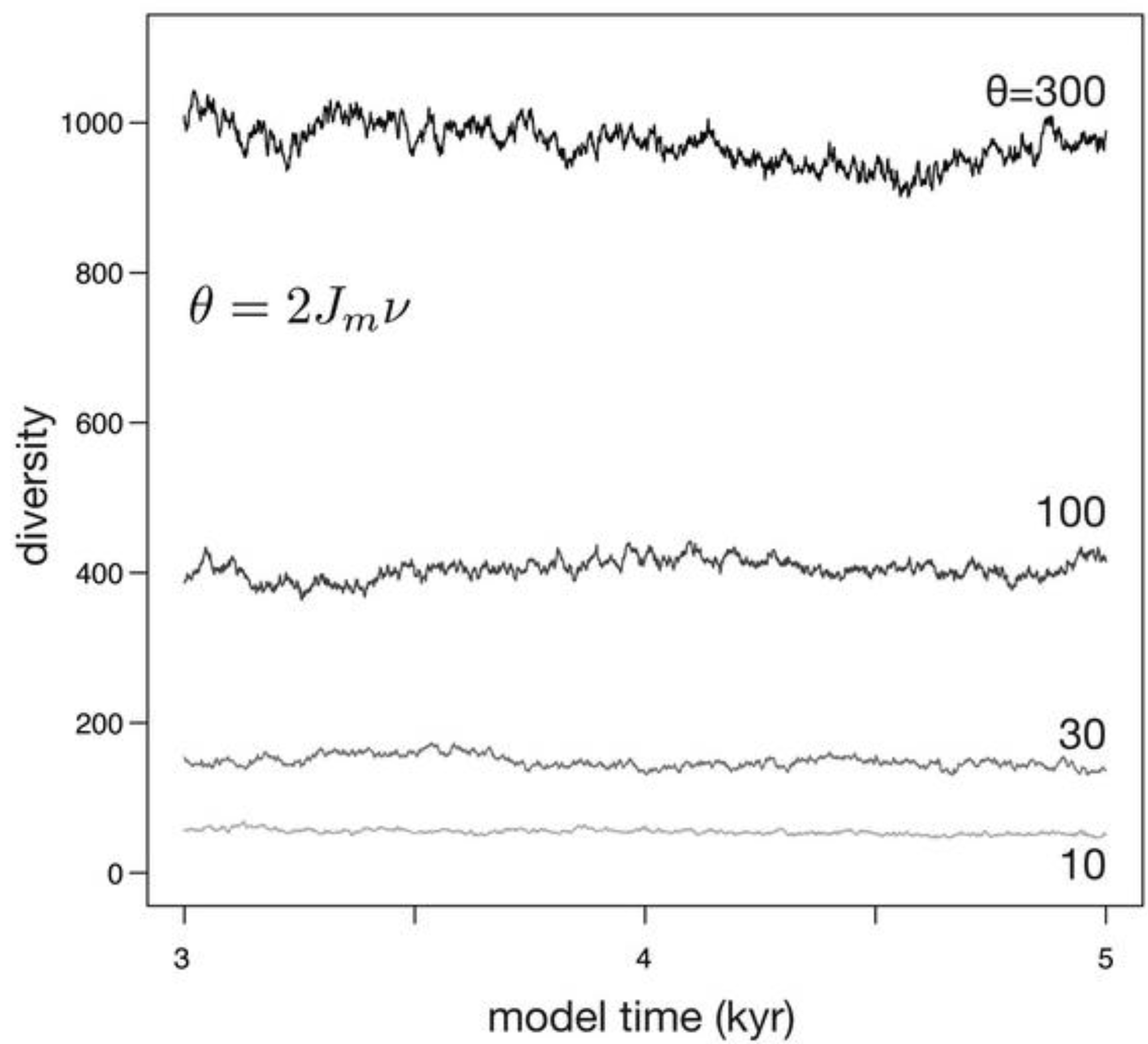
When habitat area, and therefore the number of individuals (Jm), is held fixed, diversity fluctuates around an equilibrium set by θ (Figure 4). Larger values of θ result in higher diversities, and larger values of θ also produce abundance distributions with a greater evenness. Because the death of individuals is stochastic in the simulation, as is speciation, diversity fluctuates through time. The scale of these fluctuations is roughly proportion to the equilibrium diversity, with larger fluctuations at higher values of θ. Because θ is linearly proportional to speciation rate and to the number of individuals, which is in turn the product of habitat area and the density of organisms [29], the model predicts that larger habitat areas, increased density of organisms within that habitat, and increased per-individual speciation rates should all result in larger equilibrium diversity.
Figure 4.
Simulations depicting the effect of θ on diversity when habitat area (and therefore Jm) is constant. Because Jm is constant, increases in θ are caused by increases in ν.
Figure 4.
Simulations depicting the effect of θ on diversity when habitat area (and therefore Jm) is constant. Because Jm is constant, increases in θ are caused by increases in ν.
3.2. Habitat Loss
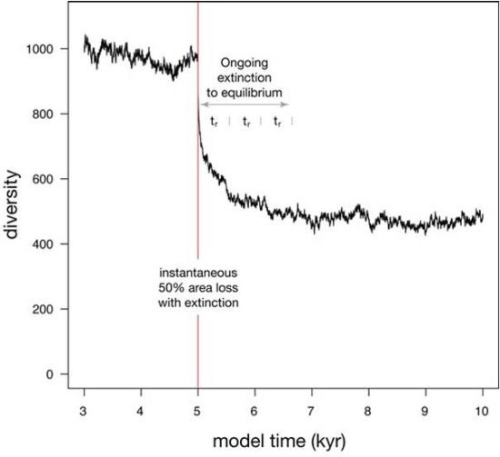
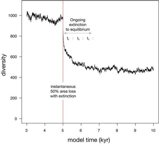
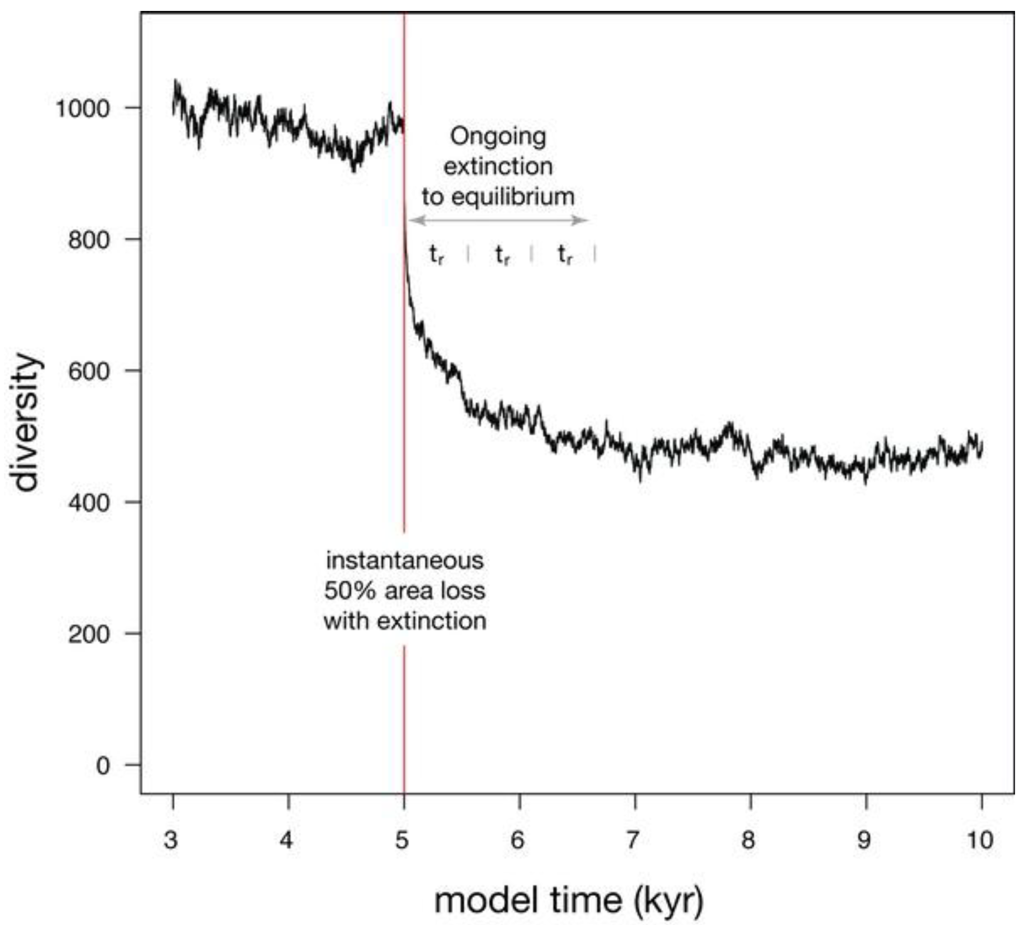
When a 50% habitat loss during a single time step is simulated (Figure 5), diversity undergoes a two-phase drop. The initial phase is instantaneous and reflects the loss of species that were confined to the area of eliminated habitat, as well as the loss of a few species that underwent stochastic extinction owing to small population size. The second phase of extinction is protracted, as diversity asymptotically approaches a new equilibrium that reflects the reduced habitat area. This asymptotic approach to a new equilibrium can be described with an exponential fit, where the time required to relax to 1/e of the original diversity (37%) is called relaxation time [26]. Relaxation is 86% complete after two relaxation times, and 95% complete after three relaxation times. In this simulation, relaxation time (tr) is 553 years, making the adjustment to the new equilibrium diversity largely complete within 1600 years.
Figure 5.
Simulation showing the effect on diversity of an instantaneous habitat loss of 50% at model time 5 kyr. 95% of extinction is complete after three relaxation times (tr).
Figure 5.
Simulation showing the effect on diversity of an instantaneous habitat loss of 50% at model time 5 kyr. 95% of extinction is complete after three relaxation times (tr).

3.2.1. Effect of Lifespan
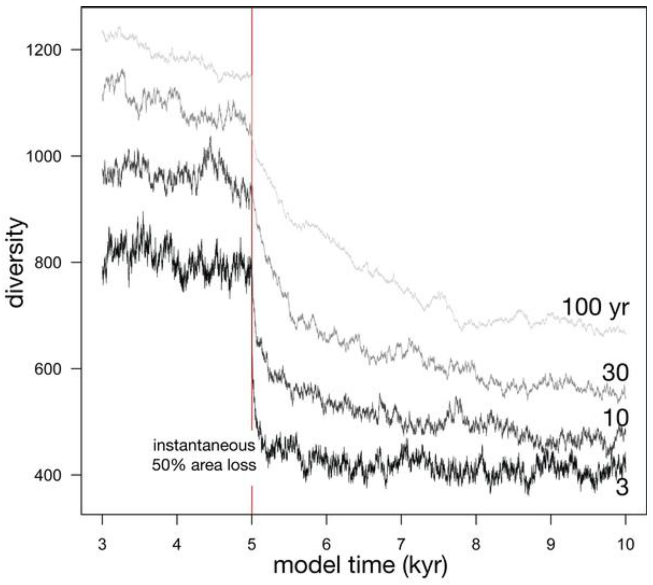
Relaxation time is partly controlled by the probability of death of an individual, the inverse of the average lifespan of an individual (Figure 6; Table 1). Shorter average lifespans, and therefore higher probabilities of death, produce a greater initial drop in diversity (compare the proportional initial diversity loss for 3 yr and 100 yr in Figure 6). Shorter average lifespans also reduce the relaxation time because of an increased turnover of individuals in every time step, speeding ecological drift. Stochastic effects can cause the equilibrium diversity to be reached more slowly or more quickly than expected; for example, the relaxation time for an average lifespan of 30 yr is slightly shorter than that for 10 years (972 years vs. 1100 years). Such stochastic effects become more important at smaller values of Jm and θ (Table 1). With longer average lifespans of 100 years, relaxation time can approach 1500 years, long on human time scales, but geologically rapid. Even with these longer relaxation times, much of the diversity drop is experienced over a shorter span, such as the first thousand years.
Figure 6.
Four simulations depicting the effect of the average lifespan of individuals on diversity before and after an instantaneous 50% habitat loss.
Figure 6.
Four simulations depicting the effect of the average lifespan of individuals on diversity before and after an instantaneous 50% habitat loss.

3.2.2. Effect of Metacommunity Size
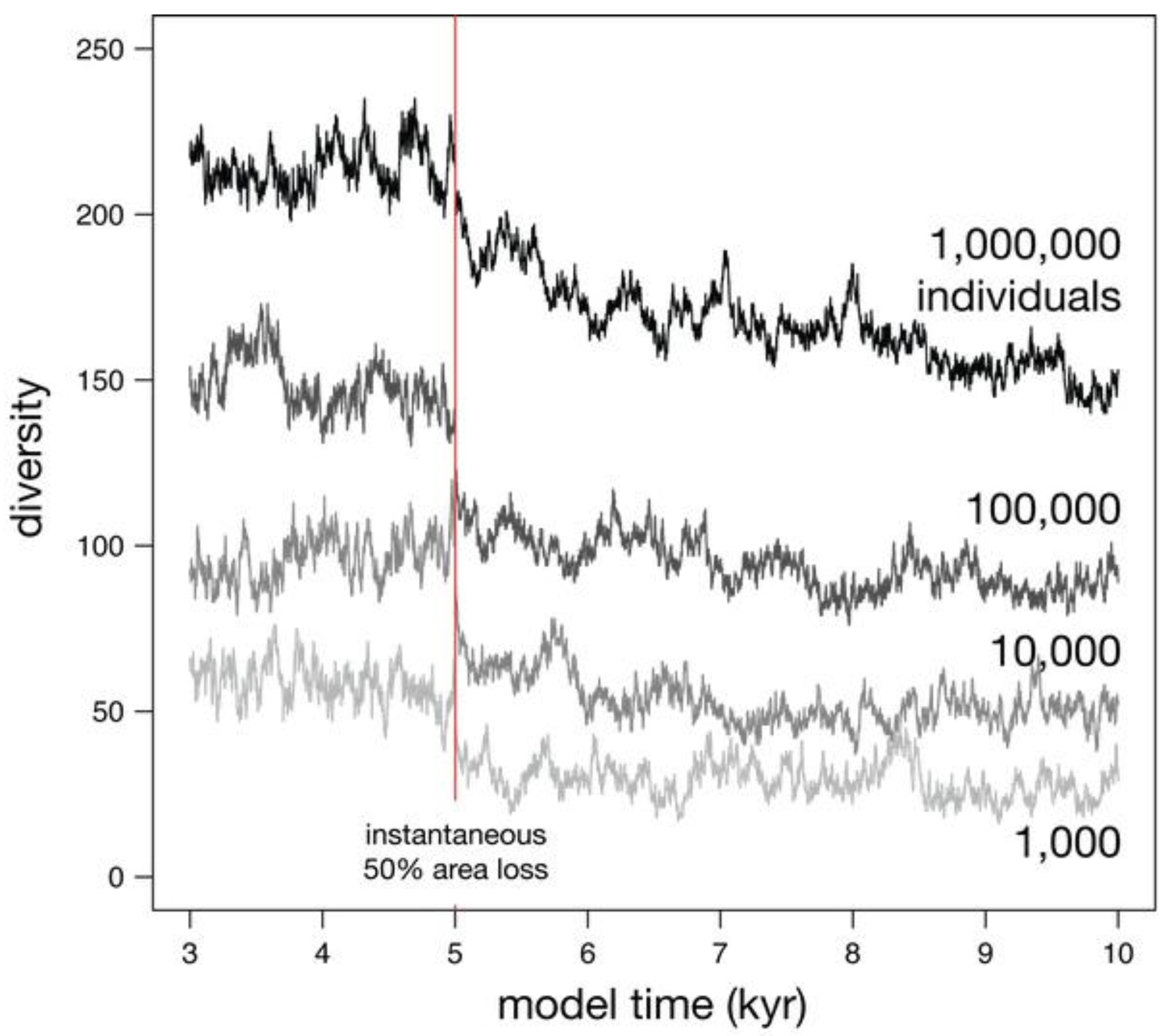
The number of individuals in the metacommunity also controls relaxation time (Jm; Figure 7; Table 1). Small metacommunities (e.g., 1,000 individuals) have short relaxation times, much less than a thousand years. Larger metacommunities (e.g., 1,000,000 individuals) can have much longer relaxation times lasting nearly 5,000 thousand years. Because most of the diversity loss occurs in the first fraction of the relaxation time, a loss of habitat area would have to be exceptionally brief to not generate extinction.
Figure 7.
Four simulations showing the effect of metacommunity size (Jm) on diversity before and after an instantaneous 50% habitat loss. The lower overall diversities compared to Figure 6 reflect the θ of 30 here, versus 300 in Figure 6.

From the perspective of the geological record, the differences among these relaxation times are small, and they are all so short that it is likely impossible to measure these directly in the fossil record in most cases, given the complexity of the stratigraphic record [34,35]. Although the differences in these relaxation times are not great, they might be manifested in the fossil record in two ways. First, large provinces should have somewhat slower relaxation times than smaller provinces, and therefore be somewhat buffered to short-lived changes in area. In this way, smaller provinces might show greater turnover and volatility as a result of sea-level change than larger provinces. Second, the metacommunity of higher trophic levels, such as predators, will generally have fewer individuals than the metacommunity of lower trophic levels, such as first-level consumers. As a result, higher trophic levels might be more acutely responsive to changes in habitat area than lower trophic levels, and this could be expressed as faster turnover rates for higher trophic levels.
3.3. Habitat Gain
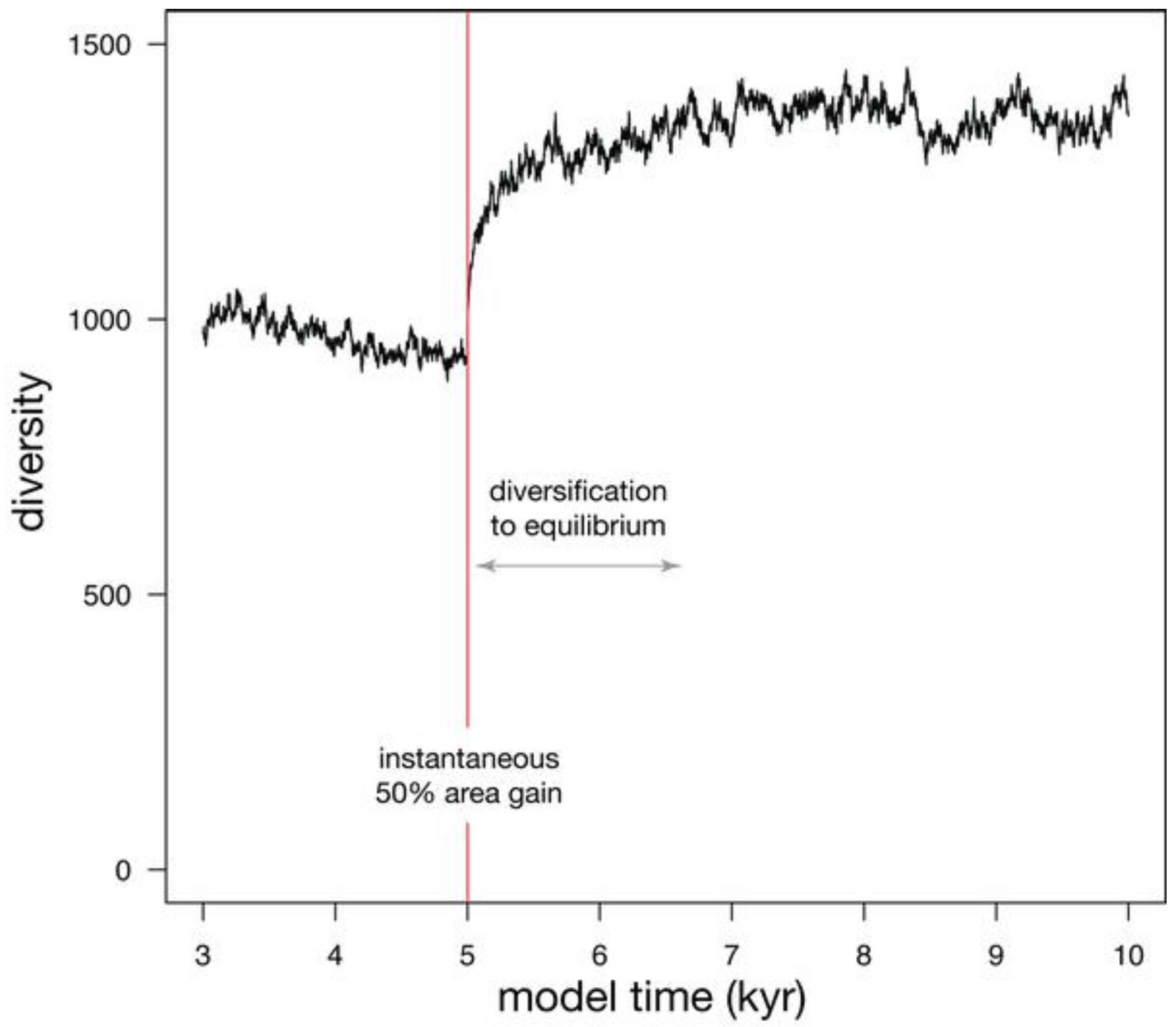
When habitat area undergoes an instantaneous 50% gain, a small pulse of speciation coincides with the area gain, and this is followed by a prolonged diversification to equilibrium (Figure 8). The initial pulse of speciation is triggered by the large number of additional unoccupied sites, each of which has a small probability of being filled by a speciation event. Although the probability of speciation is small, the large number of vacant sites allows for a small pulse of speciation.
Relaxation time during this gain in habitat area is 573 years, similar to that for habitat loss (Figure 4). Relaxation time for habitat gain is very slightly longer (573 vs. 553 years), but this difference would likely not be detectable in the geological record. Because habitat loss is accompanied by an initial extinction of endemic species, diversity would be expected to reach its equilibrium value more quickly than during habitat gain, when the initial increase in diversity is smaller.
Figure 8.
Simulation depicting the change in diversity following an instantaneous 50% gain in habitat area at 5 kyr model time.
Figure 8.
Simulation depicting the change in diversity following an instantaneous 50% gain in habitat area at 5 kyr model time.

3.4. Summary
All of these simulations indicate that neutral metacommunities should have relaxation times of no more than a few thousand years, even when the changes in habitat area are large and unrealistically abrupt as simulated here. In all cases, relaxation time is approached asymptotically with much of the diversity change experience in the early part of the relaxation period. These relaxation times are similar to or longer than estimates based on modern terrestrial faunas [26,36,37] and other models [27,38,39], suggesting that relaxation times are unlikely to be substantially longer than simulated here.
Although relaxation time increases as individuals become longer lived and as metacommunities become larger, owing to the net effects of increased area and increased density of individuals, the relaxation times remain geologically brief, suggesting that ecosystems should remain roughly in equilibrium with habitat area over geologically resolvable time scales.
4. Pleistocene Simulation
4.1. Introduction
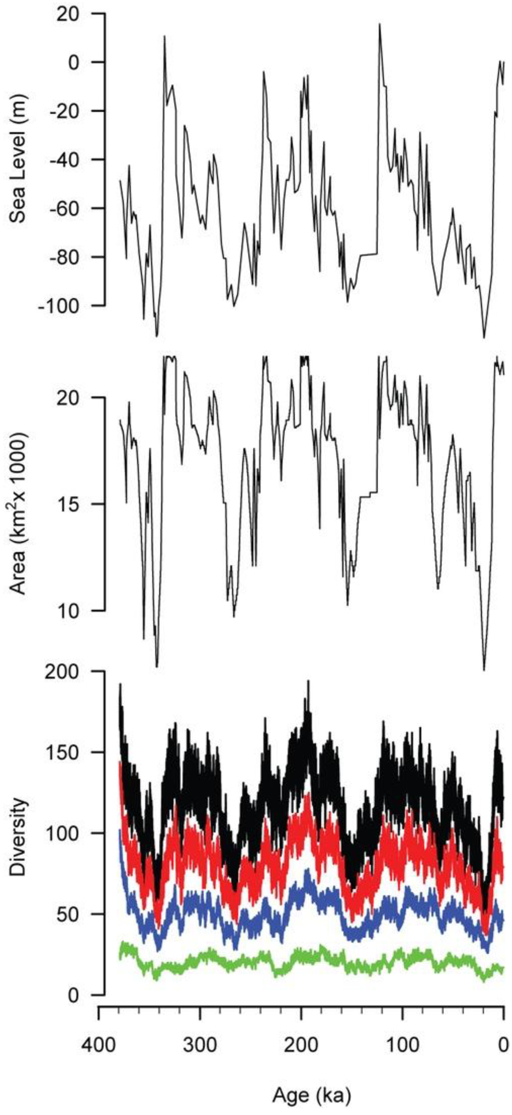
All of these simulations suggest short relaxation times, and they imply that the diversity of shallow marine faunas should have been able to closely track sea-level changes, even during times such as the Pleistocene, when sea level underwent rapid and wide changes [23,24,25]. Pleistocene sea-level changes were driven by the growth and melting of polar ice caps, which produce the highest amplitude sea-level changes over short (10s–100s kyr) geologic spans on Earth [40]. Reconstructed sea-level curves for the Pleistocene (Figure 9, top) indicate nearly continuously changing sea level with amplitudes exceeding 100 m [25].
Valentine and Jablonski [18] reported a lack of Pleistocene extinction in marine bivalves from the Californian Province, which extends from Point Conception, California (34.5°N) to Isla Cedros, Baja Mexico (28°N). Because of this, the ability of neutral communities to track continuously and widely changing sea level was tested by modeling the diversity of the Californian Province for the latest Pleistocene to today.
4.2. Model
Simulating the diversity of the Californian Province during the Pleistocene follows the same procedure as models described above, except that habitat area is allowed to change during every time step.
The position of sea level, necessary to estimate habitat area, is based on the sea-level curve of Siddall et al. [25]. Their sea-level curve was digitized and interpolated to a resolution of 1 year, providing a record of sea level back from 379 ka to the present. Such an interpolation almost certainly misses the briefest variations in habitat area, but preserves the larger amplitude, geologically detectable changes in sea level.
The area of the Californian Province was determined by measuring the area of the 0–100 m habitat corresponding to any given position of sea level. Area was measured using the National Geophysical Data Center’s ETOPO1 data set, a one arc-minute grid of global topography [6,41]. Areas were measured using the ancient sea level as the datum for the 0 m elevation and treating the topographic profile of the California shelf as unchanged. This assumption is not true in detail, but it is a reasonable approximation for the gross configuration of the margin over these relatively short time spans. The area of the 0–100 m habitat is broadly similar to the Pleistocene sea-level curve, although changes in area are often dampened compared with the sea-level signal (Figure 9, middle).
The simulation is based on annual time steps, with a metacommunity size (Jm) of 1,000,000 individuals, a θ of 30, and a probability of death of 0.1, corresponding to an average individual lifespan of 10 years. Variations on these parameters, not included here, led to similar conclusions.
4.3. Results
The simulated diversity of the Californian Province (Figure 9, bottom, black curve) broadly tracks habitat area. In particular, the three 100 kyr sea-level cycles that dominate Late Pleistocene sea level [42] are reflected in the simulated diversity history. Even some of the details of these cycles are preserved, such as the rapid rise in sea level, habitat area, and diversity around 120 ka and the slower fall in all three from 120 ka to 20 ka. Diversity also records several shorter episodes of sea-level change, such as the three peaks from 340 ka to 280 ka and the brief drop in sea level at 65 ka.
The diversity and sea-level histories differ in several ways. First, the diversity history displays more fine-scale variation, reflecting the stochastic aspect of the simulation. Second, the timing of peaks in diversity may not correspond to peaks in sea level. For example, sea level reaches a peak at 122 ka, but the local peak in diversity occurs 24 kyr later, at 98 ka. Third, the relative magnitude of peaks in diversity may not mirror the relative magnitudes of peaks in sea level. For example, three peaks in sea level at 335 ka, 315 ka, and 286 ka are successively smaller in magnitude, but the first and third of the corresponding peaks in diversity are nearly equal, and both are greater than the middle peak in diversity at 315 ka. Similarly, the peak in sea level at 256 ka is modest, but the effect on diversity is pronounced.
In the fossil record, it is impossible to sample the full biota at any given time. This is also true for modern marine environments, given the logistical difficulties involved in sampling. Limited sampling is less likely to recover rare species, and this is simulated here by imposing abundance cutoffs. For example, the black curve in Figure 9 reflects all species in the simulation, that is, those that have an abundance of 1 or more individuals, whereas the red curve reflects only those species that have an abundance of 10 or more individuals at a given time. Similarly, blue indicates species with 100 or more individuals, and green depicts those with 1000 or more individuals.
As the abundance cutoff gets larger, the correlations of diversity with area and sea level become progressively weaker. With no abundance cutoff the coefficient of determination (R2) of diversity with area and sea level are both strong (0.73 for area, 0.58 for sea level). For diversity versus area, these coefficients drop to 0.59 for a cutoff of 10, 0.38 for a cutoff of 100, and 0.21 for a cutoff of 1,000. For diversity versus sea level, the weakening is more pronounced: 0.45 for a cutoff of 10, 0.26 for a cutoff of 100, and 0.09 for a cutoff of 1,000. Time averaging in the fossil record might dampen some of the high-frequency variation in diversity, possibly improving the correlations with area and sea-level, but variations in preservation would tend to weaken these correlations.
Figure 9.
Sea level [25] for the past 379 kyr, with the area and modeled diversity of the Californian Province. The black diversity curve represents all species, red represents species with at least 10 individuals, blue is those with at least 100 individuals, and green is those with at least 1000 individuals.
5. Discussion
5.1. Departures between Diversity, Habitat Area, and Sea Level
The results from the simple area-change simulations and the Pleistocene simulation suggest that well-mixed metacommunities that operate under neutral, zero-sum dynamics should have a diversity that is nearly in equilibrium with habitat area over geological time scales, particularly at time scales greater than a few tens of thousands of years. Over shorter time scales, diversity may not be at equilibrium with habitat area, particularly following large and rapid changes in area. More generally, diversity may not be at equilibrium over shorter time scales because of the stochastic effects of death, replacement, and speciation.
Habitat area is difficult to measure in the geological record, owing to the erosion of rocks and their inaccessibility in the subsurface [28]. Although the relationship between habitat area and sea level can be markedly nonlinear [3,4,5,6], changes in sea level are commonly used to infer changes in habitat area. In the case of the Pleistocene simulation, where habitat was defined as water depths ranging from 0–100 m, habitat area broadly tracks sea level. Sea level and habitat area differ in several ways. For example, although the peak in sea level at 286 ka is slightly lower than midway between the peak at 335 ka and the low point at 266 ka, the habitat area at 286 ka is much closer to that at 335 ka than at 266 ka. Likewise, the drop in habitable area at 65 ka is much greater than the fall in sea level would suggest and the gain in area at 256 ka is much greater than the modest rise in sea level would imply.
The divergence between sea level and habitable area will weaken any correlation between sea level and diversity, and the Pleistocene simulation demonstrates this. Whereas diversity and area have a strong positive correlation, the correlation of diversity with sea level is always weaker. Although the three 100 kyr cycles in sea level are reflected in the diversity history, smaller amplitude changes in sea level may be accompanied by little or no change in diversity. For example, the 315 ka peak in sea level is barely recorded in the diversity record, and the complicated history in sea level between 237 ka and 193 ka is not reflected in diversity. Furthermore, some changes in diversity do not correspond to any change in habitable area and presumably reflect the stochastic nature of diversity changes in the simulation. For example, diversity rises to a peak at 141 ka as a result of an increase in area, but then decreases until 129 ka while habitat area is nearly constant.
5.2. Complicating Factors and Their Implications
The metacommunities simulated here are oversimplified in several regards. First, they are well-mixed and lack any spatial component, such that colonization of a vacant site depends solely on the relative abundance distribution of extant species. Second, the only ecological interaction in the simulation is competition, and the simulation is neutral in that all individuals are competitively equal. Third, the simulation follows zero-sum dynamics such that individuals occupy all available space.
Although Hubbell’s neutral theory has received much criticism, the strength of the theory lies not in that it completely describes natural systems, but in that it makes predictions that are often borne out in nature [43]. Such successful predictions suggest that more complicated models that depart from neutrality may not be necessary for predicting some aspects of metacommunities and communities. For the problem of relaxation time and the simulations presented here, the question is not whether these simulations are a complete description of nature, but whether complications might lead to longer relaxation times than predicted.
Increased species longevities are one way to lengthen relaxation time. For example, decreasing the probability of extinction would allow populations to persist during times of decreased habitat area, leading to a metapopulation diversity elevated above the equilibrium expected for the available area. Because ecological drift is more likely to lead to the extinction of small populations [29,44], mechanisms that favor the persistence of small populations will be most important for increasing relaxation time. This increased persistence could be achieved by decreasing the probability of death for individuals in species with small populations or by increasing the likelihood that species with small populations would colonize a vacated site. For example, breeding site selection can lead to increased per-capita fecundity at small population sizes [45], which would tend to increase their probability of colonizing a vacated site. It is unclear, however, how this particular mechanism would work for benthic invertebrates, many of which simply release their gametes into the water. More generally, environmental heterogeneity increases the opportunities for individual behavior to drive population dynamics [46,47], raising the possibility that benthic invertebrates may exploit these opportunities and therefore might buffer their populations from ecological drift to extinction.
Decreasing the probability of speciation is a second way to lengthen relaxation time. For example, following an increase in habitat area, a decreased probability of speciation would lengthen the time it would take for diversity to increase to the equilibrium expected for the larger area. In Hubbell’s model, speciation rate is tied directly to θ and metacommunity size (Jm), and decoupling these would allow the speciation probability to be lower, but at the expense of undermining most of the model. Changing to a more realistic speciation model, such as Hubbell’s random fission model [29] in which an existing population is split into two species during a speciation event, would likely lengthen relaxation time. In the point-mode speciation model used here, all new species begin at a population of one and are highly susceptible to ecological drift to extinction until the population builds to a sufficient size. By starting all new species at larger population levels, the probability of species extinction would be decreased and relaxation time would be increased.
More complicated models that go beyond strict neutrality will be needed to test how much such effects can increase relaxation time. The models presented here support geologically short relaxation times, in agreement with several previous actualistic and modeling studies [26,27,36,37,38,39]. Some support for brief relaxation times comes from the fossil record. One survey of mass extinctions, which include effects more complicated than simple changes in habitat area, found recovery times of 1–9 myr, but typically 1–3 myr [48]. These recovery times are longer than those suggested by the models presented here, but owing to difficulties in sampling, are likely overestimates of the true time to recovery [35]. More recent studies that explicitly consider sampling underscore geologically rapid recovery times [49,50], although these studies are at too coarse of a resolution to determine if the recovery times are as short as indicated by the models presented here.
5.3. Other Explanations for the Lack of Pleistocene Extinction
Although a long relaxation time cannot explain the lack of Pleistocene extinction in the Californian province, other explanations might. One possibility is that habitat area is not important for marine diversity [18]. Although evidence for a marine species-area relationship has been mixed [22,51,52], it seems unlikely that it does not exist in the marine realm. A lack of a species-area relationship would imply a lack of beta diversity, for which there is abundant evidence in both the modern and the fossil record [53,54,55].
A second possibility is suggested by the species studied by Valentine and Jablonski [18], who recognized the difficulty of recovering rare species. Because rare species are those that are most likely to be experience ecological drift to extinction [29], it may be that Pleistocene extinction did occur, but was limited to species so rarely found that their existence or extinction is difficult to demonstrate. The abundance cutoffs used here suggest that most faunal turnover would occur within the rare tail of the abundance distribution, and that a difficulty in collecting rare species would result in a perception of little or no extinction and relative faunal stability [56]. Numerous bulk samples may fail to recover much of the metapopulation diversity [57,58], and methods for integrating literature and museum data with collections can mitigate the difficulties of recovering rare taxa [58].
A final possibility is that local extinction did occur during Pleistocene low stands in sea level, but that species that locally went extinct were able to recolonize from deeper water or warmer southern waters [18]. Given the extensive latitudinal range shifts observed in these mollusk species [18,59], such a mechanism is likely and would create the impression that local extinction was less than it really was.
6. Conclusions
(1) Neutral models of metacommunities indicate geologically rapid responses to changes in habitat area, with relaxing times lasting a few hundred to a few thousand years, with most of the response achieved in the first quarter of that. This quasi-equilibrium with habitat area has superimposed variation in diversity caused by the stochastic effects of the probability of death, replacement, and speciation.
(2) Short relaxation times suggest that marine biotas should be in near-equilibrium with habitat area, except for large and rapid changes in area. Large metacommunities may have somewhat longer relaxation times than small metacommunities, which may be reflected by differences in relaxation time among provinces and trophic levels. Such short relaxation times suggest that Pleistocene sea-level variations should have generated marine extinction.
(3) Simulation of the Californian Province during the Pleistocene indicates good correspondence between diversity and habitat area, with a weaker correlation between diversity and sea level. These results suggest that the lack of Pleistocene marine extinction in the Californian Province is likely not the result of slow relaxation times, but is more likely the limitation of extinction to rare species and species that were able to recolonize from adjacent regions.
Acknowledgments
I thank Michael Foote, David Jablonski, and Judith Sclafani for their discussions and insights. This research was supported by National Science Foundation grant EAR-0948895.
Conflict of Interest
The author declares no conflict of interest.
References
- Harrison, C.G.A.; Brass, G.W.; Saltzman, E.S.; Sloan, J.L., II; Southam, J.; Whitman, J.M. Sea level variations, global sedimentation rates, and the hypsographic curve. Earth Planet. Sc. Lett. 1981, 54, 1–16. [Google Scholar] [CrossRef]
- Harrison, C.G.A.; Brass, G.W.; Saltzman, E.S.; Sloan, J.L., II. Continental hypsography. Tectonics 1983, 2, 357–377. [Google Scholar] [CrossRef]
- Wyatt, A.R. Relationship between continental area and elevation. Nature 1984, 311, 370–372. [Google Scholar] [CrossRef]
- Wyatt, A.R. Shallow water areas in space and time. J. Geol. Soc. London 1987, 144, 115–120. [Google Scholar] [CrossRef]
- Algeo, T.J.; Wilkinson, B.H. Modern and ancient continental hyposometries. J. Geol. Soc. London 1991, 148, 643–653. [Google Scholar] [CrossRef]
- Holland, S.M. Sea level change and the area of shallow-marine habitat: implications for marine biodiversity. Paleobiology 2012, 38, 205–217. [Google Scholar] [CrossRef]
- Chamberlin, T.C. Diastrophism as the ultimate basis of correlation. J. Geol. 1909, 17, 689–693. [Google Scholar]
- Moore, R.C. Evolution of late Paleozoic invertebrates in response to major oscillations of shallow seas. Bull. Harv. Mus. Comparat. Zool. 1954, 122, 259–286. [Google Scholar]
- Newell, N.D. Revolutions in the history of life. Geol. Soc. Am. 1967, 89, 63–91. [Google Scholar] [CrossRef]
- Flessa, K.W.; Sepkoski, J.J., Jr. On the relationship between Phanerozoic diversity and changes in habitable area. Paleobiology 1978, 4, 359–366. [Google Scholar]
- Bayer, U.; McGhee, G.R. Evolution in marginal epicontinental basins: The role of phylogenetic and ecologic factors (Ammonite replacements in the German Lower and Middle Jurassic). In Sedimentary and Evolutionary Cycles; Bayer, U., Seilacher, A., Eds.; Springer-Verlag: New York, NY, USA, 1985; pp. 164–220. [Google Scholar]
- Jablonski, D. Causes and consequences of mass extinctions: A comparative approach. In Dynamics of Extinction; Elliot, D.K., Ed.; John Wiley & Sons: New York, NY, USA, 1986; pp. 183–229. [Google Scholar]
- Hallam, A. Radiations and extinctions in relation to environmental change in the marine Lower Jurassic of northwest Europe. Paleobiology 1987, 13, 152–168. [Google Scholar]
- Hallam, A. Phanerozoic. Sea-level Changes; Columbia University Press: New York, NY, USA, 1992. [Google Scholar]
- Brett, C.E. Sequence stratigraphy, paleoecology, and evolution: Biotic clues and responses to sea-level fluctuations. Palaios 1998, 13, 241–262. [Google Scholar] [CrossRef]
- Raup, D.M. Species diversity in the Phanerozoic: An interpretation. Paleobiology 1976, 4, 1–15. [Google Scholar]
- Wise, K.P.; Schopf, T.J.M. Was marine faunal diversity in the Pleistocene affected by changes in sea level? Paleobiology 1981, 7, 394–399. [Google Scholar]
- Valentine, J.W.; Jablonski, D. Biotic effects of sea level change: The Pleistocene test. J. Geophys. Res. 1991, 96, 6873–6878. [Google Scholar]
- McGhee, G.R., Jr. Extinction and diversification in the Devonian brachiopoda of New York state: No correlation with sea-level? Hist. Biol. 1991, 5, 215–227. [Google Scholar]
- McGhee, G.R., Jr. Evolutionary biology of the Devonian brachiopoda of New York state: No correlation with rate of change of sea-level? Lethaia 1992, 25, 165–172. [Google Scholar] [CrossRef]
- Crampton, J.S.; Foote, M.; Beu, A.G.; Maxwell, P.A.; Cooper, R.A.; Matcham, I.; Marshall, B.A.; Jones, C.M. The ark was full! Constant to declining cenozoic shallow marine biodiversity on an isolated midlatitude continent. Paleobiology 2006, 32, 509–532. [Google Scholar] [CrossRef]
- Peters, S.E.; Ausich, W.I. A sampling-adjusted macroevolutionary history for Ordovician–Early Silurian crinoids. Paleobiology 2008, 34, 104–116. [Google Scholar] [CrossRef]
- Lisiecki, L.E.; Raymo, M.R. A Pliocene-Pleistocene stack of 57 globally distributed benthic δ18O records. Paleoceanography 2005. [Google Scholar] [CrossRef]
- Miller, K.G.; Kominz, M.; Browning, J.V.; Wright, J.D.; Mountain, G.S.; Katz, M.E.; Sugarman, P.J.; Cramer, B.S.; Christie-Blick, N.; Pekar, S.F. The Phanerozoic record of global sea-level change. Science 2005, 310, 1293–1298. [Google Scholar] [CrossRef]
- Siddall, M.; Rohling, E.J.; Almogi-Labin, A.; Hemleben, C.; Meischner, D.; Schmelzer, I.; Smeed, D.A. Sea-level fluctuations during the last glacial cycle. Nature 2003, 423, 853–858. [Google Scholar]
- Diamond, J.M. Biogeographic kinetics: estimation of relaxation times for avifaunas of Southwest Pacific Islands. Proc. Natl. Acad. Sci. USA 1972, 69, 3199–3203. [Google Scholar]
- Tilman, D.; May, R.M.; Lehman, C.L.; Nowak, M.A. Habitat destruction and the extinction debt. Nature 1994, 371, 65–66. [Google Scholar]
- Smith, A.B.; Gale, A.S.; Monks, N.E.A. Sea-level change and rock-record bias in the Cretaceous: a problem for extinction and biodiversity studies. Paleobiology 2001, 27, 241–253. [Google Scholar] [CrossRef]
- Hubbell, S.P. The Unified Neutral Theory of Biodiversity and Biogeography; Monographs in Population Biology 32; Princeton University Press: Princeton, NJ, USA, 2001. [Google Scholar]
- R Core Team, R: A Language and Environment for Statistical Computing; R Foundation for Statistical Computing: Vienna, Austria, 2012.
- Hankin, R. Introducing untb, an R package for simulating ecological drift under the unified neutral theory of biodiversity. J. Stat. Softw. 2007, 22, 1–15. [Google Scholar]
- Thorson, G. Bottom communities (sublittoral or shallow shelf). Geol. Soc. Am. Mem. 1957, 67, 461–534. [Google Scholar]
- Abele, D.; Brey, T.; Philipp, E. Bivalve models of aging and the determination of molluscan lifespans. Exp. Gerontol. 2009, 44, 307–315. [Google Scholar] [CrossRef] [Green Version]
- Holland, S.M. The stratigraphic distribution of fossils. Paleobiolog 1995, 21, 92–109. [Google Scholar]
- Holland, S.M. The quality of the fossil record—a sequence stratigraphic perspective. In Deep Time: Paleobiology’s Perspective; Erwin, D.H., Wing, S.L., Eds.; The Paleontological Society: Lawrence, KS, USA, 2000; pp. 148–168. [Google Scholar]
- Boecklin, W.J.; Simberloff, D. Area-based extinction models in conservation. In Dynamics of Extinction; Elliot, D.K., Ed.; John Wiley: New York, NY, USA, 1986; pp. 247–272. [Google Scholar]
- Vellend, M.; Verheyen, K.; Jacquemyn, H.; Kolb, A.; van Calster, H.; Peterken, G.; Hermy, M. Extinction debt of forest plants persists for more than a century following habitat fragmentation. Ecology 2006, 87, 542–548. [Google Scholar]
- Halley, J.M.; Iwasa, Y. Neutral theory as a predictor of avifaunal extinctions after habitat loss. Proc. Natl. Acad. Sci. USA 2011, 108, 2316–2321. [Google Scholar] [CrossRef]
- Mouquet, N.; Matthiessen, B.; Miller, T. Gonzalez, Extinction debt in source-sink metacommunities. PloS One 2011, 6, e17567. [Google Scholar] [CrossRef] [Green Version]
- Revelle, R. Sea-Level Change; National Academy Press: Washington, DC, 1990. [Google Scholar]
- ETOPO1 Global Relief Model. Available online: http://www.ngdc.noaa.gov/mgg/global/global.html/ (accessed on 1 April 2013).
- Berger, A. Pleistocene climatic variability at astronomical frequencies. Quatern. Int. 1989, 2, 1–14. [Google Scholar] [CrossRef]
- Rosindell, J.; Hubbell, S.P.; Etienne, R.S. The Unified Neutral Theory of Biodiversity and Biogeography at age ten. Trends Ecol. Evol. 2011, 26, 340–348. [Google Scholar] [CrossRef]
- Goodman, D. The demography of chance extinction. In Viable Populations for Conservation; Soulé, M., Ed.; Cambridge University Press: Cambridge, UK, 1987; pp. 11–34. [Google Scholar]
- McPeek, M.A.; Rodenhouse, N.L.; Holmes, R.T.; Sherry, T.W. A general model of site-dependent population regulation: population-level regulation without individual-level interactions. Oikos 2001, 94, 417–424. [Google Scholar]
- Holt, R.D. Population dynamics in two-patch environments: some anomalous consequences of an optimal habitat distribution. Theor. Popul. Biol. 1985, 28, 181–208. [Google Scholar] [CrossRef]
- Morris, D.W. Habitat-dependent population regulation and community structure. Evol. Ecol. 1988, 2, 253–269. [Google Scholar] [CrossRef]
- Erwin, D.H. The end and the beginning: Recoveries from mass extinctions. Trends Ecol. Evol. 1998, 13, 344–349. [Google Scholar] [CrossRef]
- Erwin, D.H. Lessons from the past: Biotic recoveries from mass extinctions. Proc. Natl. Acad. Sci. USA 2001, 98, 5399–5403. [Google Scholar] [CrossRef]
- Alroy, J.; Aberhan, M.; Bottjer, D.J.; Foote, M.; Fürsich, F.T.; Harries, P.J.; Hendy, A.J.W.; Holland, S.M.; Ivany, L.C.; Kiessling, W.; et al. Phanerozoic trends in the global diversity of marine invertebrates. Science 2008, 321, 97–100. [Google Scholar] [CrossRef]
- Stanley, S.M. Marine mass extinction: A dominant role for temperature. In Extinctions; Nitecki, M.H., Ed.; University of Chicago Press: Chicago, IL, USA, 1984; pp. 69–117. [Google Scholar]
- Schopf, T.J.M.; Fisher, J.B.; Smith, C.A.F., III. Is the marine latitudinal diversity gradient merely another example of the species-area curve? In Marine Organisms: Genetics, Ecology, and Evolution; Battaglia, B., Beardmore, J.A., Eds.; Plenum: New York, NY, USA, 1978; pp. 365–386. [Google Scholar]
- Kowalewski, M.; Gürs, K.; Nebelsick, J.H.; Oschmann, W.; Piller, W.E.; Hoffmeister, A.P. Multivariate hierarchical analyses of miocene mollusk assemblages of europe: Palaeogeographic, palaeoecological, and biostratigraphic implications. Geol. Soc. Am. Bull. 2002, 114, 239–256. [Google Scholar]
- Okuda, T.; Noda, T.; Yamamoto, T.; Ito, N.; Nakaoka, M. Latitudinal gradient of species diversity: Multi-scale variability in rocky intertidal sessile assemblages along the northwestern Pacific coast. Popul. Ecol. 2004, 46, 159–170. [Google Scholar]
- Patzkowsky, M.E.; Holland, S.M. Diversity partitioning of a Late Ordovician marine biotic invasion: Controls on diversity in regional ecosystems. Paleobiology 2007, 33, 295–309. [Google Scholar] [CrossRef]
- McKinney, M.L.; Lockwood, J.L.; Frederick, D.R. Does ecosystem and evolutionary stability include rare species? Palaeogeogr. Palaeocl. 1996, 127, 191–207. [Google Scholar] [CrossRef]
- Holland, S.M.; Miller, A.I.; Meyer, D.L.; Dattilo, B.F. The detection and importance of subtle biofacies within a single lithofacies: The Upper Ordovician Kope Formation of the Cincinnati, Ohio region. Palaios 2001, 16, 205–217. [Google Scholar] [CrossRef]
- Harnik, P.G. Unveiling rare diversity by integrating museum, literature, and field data. Paleobiology 2009, 35, 190–208. [Google Scholar] [CrossRef]
- Roy, K.; Jablonski, D.; Valentine, J.W. Thermally anomalous assemblages revisited: Patterns in the extraprovincial latitudinal range shifts of Pleistocene marine mollusks. Geology 1995, 23, 1071–1074. [Google Scholar] [CrossRef]
© 2013 by the authors; licensee MDPI, Basel, Switzerland. This article is an open access article distributed under the terms and conditions of the Creative Commons Attribution license (http://creativecommons.org/licenses/by/3.0/).
Share and Cite
MDPI and ACS Style
Holland, S.M. Relaxation Time and the Problem of the Pleistocene. Diversity 2013, 5, 276-292. https://doi.org/10.3390/d5020276
AMA Style
Holland SM. Relaxation Time and the Problem of the Pleistocene. Diversity. 2013; 5(2):276-292. https://doi.org/10.3390/d5020276
Chicago/Turabian StyleHolland, Steven M. 2013. "Relaxation Time and the Problem of the Pleistocene" Diversity 5, no. 2: 276-292. https://doi.org/10.3390/d5020276