New Transcorrelated Method Improving the Feasibility of Explicitly Correlated Calculations

1
Graduate School of Human Informatics, Nagoya University, Chikusa-ku Nagoya 464-8601 Japan
2
The Graduate University for Advanced Sciences, Myodaiji, Okazaki 444-8585 Japan
*
Author to whom correspondence should be addressed.
Int. J. Mol. Sci. 2002, 3(5), 459-474; https://doi.org/10.3390/i3050459
Submission received: 18 September 2001
/
Accepted: 14 December 2001
/
Published: 31 May 2002
(This article belongs to the Special Issue Recent Advances in Coupled Cluster Theory)
Abstract
:We recently developed an explicitly correlated method using the transcorrelated Hamiltonian, which is preliminarily parameterized in such a way that the Coulomb repulsion is compensated at short inter-electronic distances. The extra part of the effective Hamiltonian features short-ranged, size-consistent, and state-universal. The localized and frozen nature of the correlation factor makes the enormous three-body interaction less important and enables us to bypass the complex nonlinear optimization. We review the basic strategy of the method mainly focusing on the applications to single-reference many electron theories using modified Møller-Plesset partitioning and biorthogonal orbitals. Benchmark calculations are performed for 10-electron systems with a series of basis sets.
1. INTRODUCTION
In modern ab initio quantum chemistry, the convergence of calculations with the size of one-electronic basis functions is crucial for predicting reliable energetics and molecular properties. It has been, however, recognized that an enormous basis with high angular momentum functions is required to achieve chemical accuracy of a few kcal/mol in total energies. The slow convergence of the dynamic correlation effects is a direct consequence of the inability of describing the correlation cusp [1] with one-electronic basis. Various alternatives incorporating the inter-electronic coordinate explicitly have been suggested to ameliorate this feature. With the objectives of many electronic systems, the Gaussian-type geminals (GTGs) [2,3] have been used in many places. Especially, Szalewicz and coworkers have used GTG successfully for accurate calculations of correlation energies in their series of papers [4,5]. Although the function form is not suitable from the viewpoint of the cusp condition, the methods with GTGs have demonstrated the efficiency [6,7] to give correlation energies to μHartree accuracy, as shown in the recent result of Cencek and Rychlewski [8]. This situation is comprehensible by evaluating the motion of pair-electrons in three-dimension, i.e. the gain from the cusp around a fixed electron scales as
while the Coulomb repulsion factorize no more than .
The R12 method [9,10,11,12] developed by Klopper, Kutzelnigg and coworkers is another original scheme, which incorporates the linear behavior to describe the dynamic correlation effects. The method introduces systematic approximations, which bypass the explicit treatment of the so-called “difficult integrals”. The approximations become more reliable as the one-electronic expansion set, which is formally assumed to be complete, gets sufficiently large. The R12 ansatz has provided highly-reliable correlated methods. Especially, the R12 coupled-cluster (CC) method developed by Noga et al. [13,14,15] achieves the chemical accuracy both in the quality of the Hilbert space to describe the electronic motions and the sophistication of the correlated method. One disadvantage of the method is that the theoretical construction is intricate because of the wave operator form and the approximation to the various difficult integrals. The long-range nature of the linear behavior is another element that makes a scalable treatment complicated. Persson and Taylor developed another method related with the R12 theory [16]. They fit the linear function using GTG to avoid the nonlinear optimization for GTG. The approach aims at calculations of modest accuracy in comparison with the previous GTG theories, i.e. sub-mHartree accuracy for valence correlations within the framework of the second order Møller-Plesset perturbation (MP2) theory.
All of the above-mentioned methods use functions with inter-electronic coordinate and orthogonal projectors. In other words, the explicitly correlated wave operators are not commutable with the Coulomb interactions in the complete basis limit. This property is the main source complicating the explicitly correlated methods. The transcorrelated method [17,18] developed by Boys and Handy is on the basis of symmetric correlation factor commutable with the Coulomb interaction. As a result, the effective Hamiltonian, the so-called transcorrelated Hamiltonian, includes at most three-body effective interactions. In recent publications, we developed a method which uses the transcorrelated Hamiltonian especially for pair-wise short-range collisions [19,20,21]. The method does not include any nonlinear optimization of the correlation factor, which is present in the original transcorrelated method. Instead, we deal with the long-range correlation in terms of the usual configuration interaction (CI)-type expansion with one-electronic functions.
In this paper, we briefly review the basic ideas of our transcorrelated method in the next section. The manipulations of molecular integrals are explained in Sec. 3. We formulate the application to single-reference methods including the linearized CC (LCC) method in Sec. 4. Some benchmark calculations of 10-electronic systems are given in Sec. 5. Conclusions are depicted in Sec. 6.
2. TRANSCORRELATED HAMILTONIAN
In our transcorrelated method, the exact wave function is expressed as a product of a symmetric correlation factor, , and an anti-symmetrized CI-type wave function, [19],
where is assumed to be a sum of two-electron functions (geminals),
We aim at improving the convergence of CI treating the cusp behavior in the vicinity, , with the factor. Since the vicinity is dominated by the Coulomb repulsion, the simplest choice for the purpose is to employ a geminal, which is also spherically symmetric,
The similarity transformed effective Hamiltonian terminating at the double commutator [17,18],
is a sum of the original Hamiltonian and the effective two- and three-electronic interactions,
The two-electronic part consists of the terms linear and quadratic to the factor,
and the three-electron operator is given by
The operators, and , are anti-symmetric and symmetric, respectively. The latter can be combined with the Coulomb one in a practical computer code. It is possible to replace the operators by the averaged ones,
This simplifies the algebraic manipulations, which appear in correlated wave function methods.
The geminal is parameterized under the following conditions. Firstly, the Coulomb singularity is compensated by the effective potential in . It is known that the condition leads to the linear behavior of the geminal, which enables us to express the Coulomb cusp explicitly with a finite number of one-electronic functions. Secondly, we localize the geminal. The linear behavior is generally adequate only in the vicinity, , where the Coulomb potential is dominating the inter-electronic shape. We maintain the usual CI picture in the long-range behavior of the correlated wave function. For practical applications, the geminal is expressed as a sum of Gaussian-type functions,
and the parameters are determined using a least square fit for the approximate equality,
where is a short-range weight function [19]. We have used an additional Gaussian for the weight function. The above condition involves no more than the derivatives of . An additional requirement is therefore the geminal converges to zero at the infinite distance. This is automatically fulfilled with the present use of Gaussian-type functions. The choice of the localized geminal is crucial because the number of integrals increases only linearly with the size of the molecule. Moreover, the three-body interaction, , becomes less important because of the decreasing probability of finding three electrons in the geminal radius. This is consistent with the localized nature of the dynamic correlation effects.
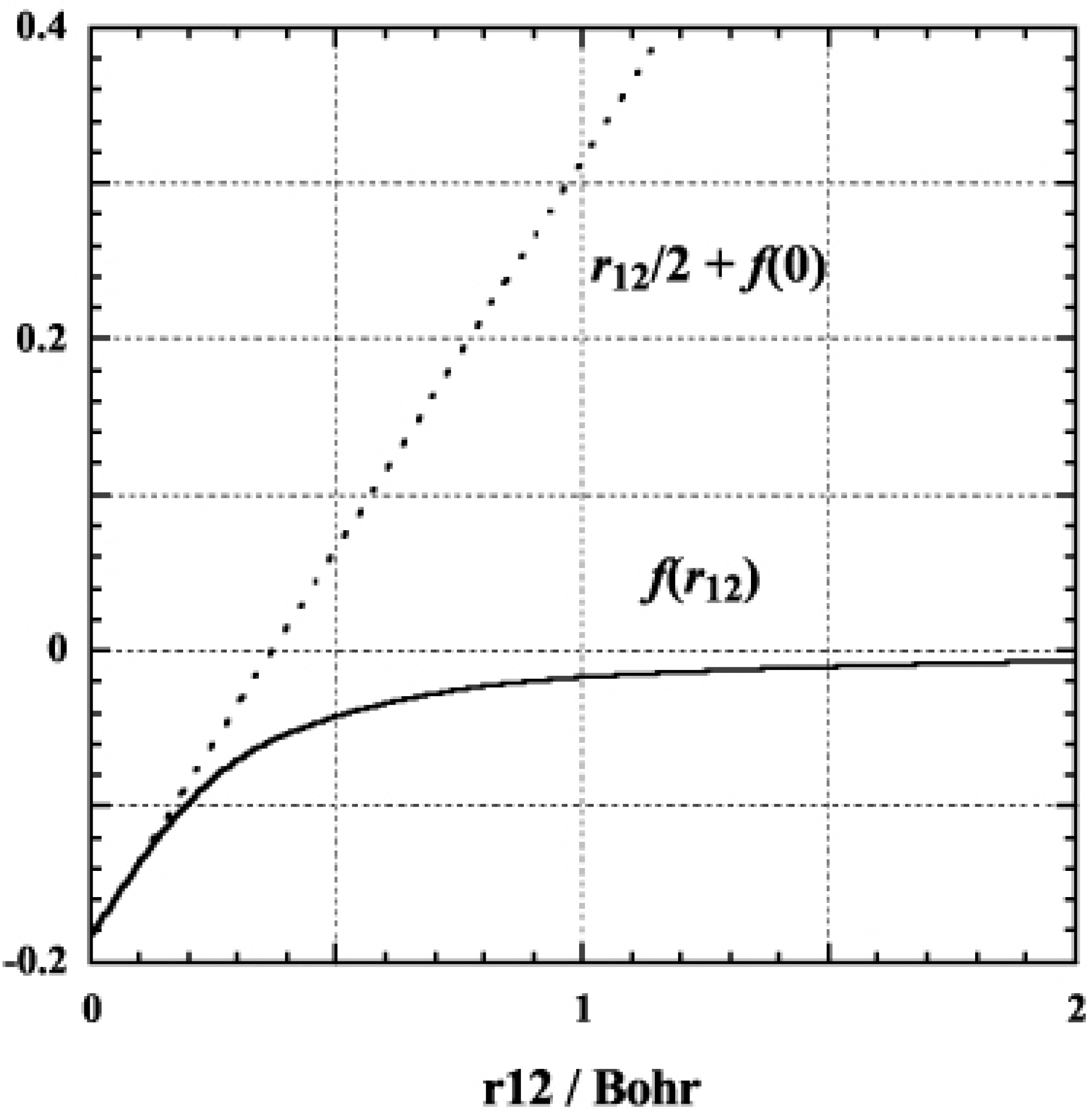
We use the tight geminal consisting of 10 Gaussian-type functions throughout of this paper. The exponents are determined as an even-tempered sequence of the function with the exponents between 904000.0 and 0.12, and that of the weight Gaussian is chosen to be 20.0. Fig.1 shows the shape of the geminal. The geminal coincides with the linear behavior around the origin. It will be shown that the introduction of the short-range correlation factor significantly improves the description of the dynamic correlation effects in latter sections.
3. INTEGRALS IN THE TRANSCORRELATED METHOD
The three-electron integrals, , are expressed in closed form in terms of recurrence relations [20]. The explicit treatment of the integrals, however, prohibits the application of the transcorrelated Hamiltonian to large molecular systems despite the use of the short-range geminal. The best feature of the present approach is that the three-body contribution is less important to make
![Ijms 03 00459 g001]() the transcorrelated method feasible by using completeness insertions. One of such expressions is in the form,
The expression requires all Cartesian components of the integrals, , to which the point group symmetry cannot be applied. If the three basis functions, p, q and t, are s-orbitals with a coincident function center, only the p-component of the v function survives. This means that expansion functions, whose angular momentums are higher than the atomic orbitals by 1, are necessary in equation (3.1). Alternatively, we fall back on the idea of the operator identity,
where and are given in the occupation number representation by
and the subscript, , at the commutator denotes single contractions. Using the fact that is commutable with in the complete basis limit about the second electronic coordinate, we obtain the approximate expression for the three-electron integrals,
This expression features that the integrals, , are only required besides the anti-symmetric part of . The point group symmetry is applicable to the integrals. Since the operator, , does not increase the angular momentum of orbitals, the convergence of the completeness insertion of equation (3.5) is superior to the previous expression, equation (3.1). It is also possible to derive another expression using the averaged operator, , rather than as
Both of the expressions with and are exact in the complete basis limit. We examine the first in this work.
the transcorrelated method feasible by using completeness insertions. One of such expressions is in the form,
The expression requires all Cartesian components of the integrals, , to which the point group symmetry cannot be applied. If the three basis functions, p, q and t, are s-orbitals with a coincident function center, only the p-component of the v function survives. This means that expansion functions, whose angular momentums are higher than the atomic orbitals by 1, are necessary in equation (3.1). Alternatively, we fall back on the idea of the operator identity,
where and are given in the occupation number representation by
and the subscript, , at the commutator denotes single contractions. Using the fact that is commutable with in the complete basis limit about the second electronic coordinate, we obtain the approximate expression for the three-electron integrals,
This expression features that the integrals, , are only required besides the anti-symmetric part of . The point group symmetry is applicable to the integrals. Since the operator, , does not increase the angular momentum of orbitals, the convergence of the completeness insertion of equation (3.5) is superior to the previous expression, equation (3.1). It is also possible to derive another expression using the averaged operator, , rather than as
Both of the expressions with and are exact in the complete basis limit. We examine the first in this work.
Figure 1.
The shape of the geminal, , used in this work (full line). The dotted line denotes the linear behavior, required to balance the Coulomb repulsion around the origin.
Figure 1.
The shape of the geminal, , used in this work (full line). The dotted line denotes the linear behavior, required to balance the Coulomb repulsion around the origin.
The present transcorrelated method requires the three different kinds of two-electron integrals, , and . Assuming the basis functions to be primitive Gaussian-type functions and using the Laplace transform of the Coulomb operator, the electron repulsion integrals are written in the form,
where are coefficients dependent only on the exponents and positions of the four basis functions, the zero indices means s-type functions, is the Gaussian function with the exponent, ,
the function, , is given by
and is a parameter which is a function of the four primitive exponents. The index, , runs up to the sum of maximum angular momentums of the basis functions. For each point, , the coefficients for the increments of angular momentums are independent in each Cartesian axis. The polynomial, , is therefore expressed as a product of the Cartesian contributions,
The Cartesian components, , can be calculated using recurrence relations [22].
Similarly, the integrals, , are expressed as,
The recurrence relation [22] shows that the integrals for the operators, and , which are more complex, also reduce to the kind of integrals, . The maximum value, , increases by 2 because of the differentiations. For the operator, , we introduce the integrals,
where denote sums of exponents of the geminal, . Using the relations,
it is shown that the integrals for reduce to the combination of the type of the integrals, . One notes that the coefficients, , which are dependent only on the angular momentums and the positions of the orbital quartet, are shared by all types of the integrals.
We express the functions, , using polynomials as
where and are the root and the weight for the point, , which runs over the same range as . The functions, and , are connected through a linear transformation predetermined for . In the Rys quadrature method [23,24], both of the roots and weights are chosen to be variables reducing the number of root points to be larger than rather than . We do not employ this convention but use fixed roots for all operators, . Once the integrals are written in the discrete polynomials, the summation over
is expressed as a product of Cartesian components. For instance, the electron repulsion integrals become in the form,
The above procedure enables us to calculate the integrals for different two-electronic operators simultaneously by changing the weight, , after setting up the common quantities, .
4. APPLICATION TO SINGLE-REFERENCE MANY ELECTRON THEORIES
Basically, the application of the transcorrelated method is straightforward; the original Hamiltonian, , is replaced by the transcorrelated one, , in the usual ab initio theories. The transcorrelated Hamiltonian is, however, nonhermite including weak three-body interactions. This property gives rise to a few variations in formulating single reference theories. Throughout this paper, we use the notations, and for virtual and occupied orbitals within a given basis set, respectively. Our first method employs a coincident vacuum determinant for the bra and ket states in the CC equations,
where is a single-determinant vacuum, denotes particle-hole excitation operators with respect to the vacuum, and means the connected entity of the operators. A suitable partitioning of the Hamiltonian leads to an order-by-order expansion of the wave operator. Since our transcorrelated Hamiltonian is designed to coincide with the long-range behavior of the original Coulomb operator, the usual Hartree-Fock (HF) model Hamiltonian in the MP perturbation theory is a good starting point for the expansion [19],
choosing to be the HF determinant for the original Hamiltonian. One notes that the new perturbation, , is nearly free from the Coulomb singularity. We therefore can anticipate that the perturbational series converges quicker than the usual MP one.
The above argument is not the case for electrons around nuclei especially when we introduce an approximation to the CC method. The operator dependent on the momentum of the anti-symmetric part, , becomes significant for core electrons of heavy atomic elements. In the present application, we preliminarily treat the orbital relaxation with the pseudo-orbital equation, excluding the expensive but less important three-body contribution from the iterative loop,
The subsequent connected singles and doubles are restored order-by-order approximately using the LCC equation known to be CEPA0 [25,26],
The similarity transformed Hamiltonian,
analogous to the one, which appeared in the treatment of CCSD amplitudes [27,28], retains the operator rank of the transcorrelated Hamiltonian. The procedure is adequate especially for a molecule consisting of light atomic elements.
Another option, which gives results similar to those of the above-mentioned modified MP partitioning with the pseudo-orbital equation but uses more optimized reference functions, is based on biorthogonal one-electronic basis sets [29,30]. For a while, we denote the orbitals in the one-electronic sets as and , respectively. The biorthogonality condition is given by
Creation and annihilation operators are defined using the field operators as
Operators are expressed in the second quantized form of the biorthogonal set, like
Since the anti-commutation relation holds for the new creation and annihilation operators,
the Wick theorem and accordingly the usual diagrammatic technique can be used for manipulating operators in the biorthogonal form.
We introduce separate single-reference vacua consisting of biorthogonal orbitals, and . The canonical orbitals are determined self-consistently using the approximate Fock operator [21],
where means anti-symmetrized integrals. We solve the LCCSD equation,
iteratively with the zeroth order Hamiltonian, , where we define the excitation and deexciation operators with respect to the right vacuum, and , and the cluster operator, .
It should be noted that the present methods do not alter the original scaling of the correlated methods. The pseudo-orbital and biothogonal self-consistent field (SCF) methods, which exclude the contribution of , are driven in the atomic orbital basis. This gives rise to the formal scaling as the usual SCF method. The subsequent LCCSD code is commonly used in both of the methods substituting the individual transformed integrals and energy denominators. The double contractions of and the two-electron operators in the transcorrelated Hamiltonian, , and , become the rate-determining steps at this level. These scale as at most as the conventional CCSD and LCCSD methods for and denoting the numbers of virtual and occupied orbitals, respectively. The effect of the connected triples from is negligibly small owing to the localized nature of the correlation factor.
5. RESULT AND DISCUSSION
We examine the efficiency of the transcorrelated method in the calculations of the typical 10-electronic systems, CH3, NH3, H2O, HF and Ne. We first check the convergence of the correlation energies for H2O and Ne with the correlation consistent basis sets of Dunning [31], cc-pVXZ (X = D, T, Q and 5). The basis functions are used as primitives to increase the flexibility. Each basis set is further augmented with the d- f- and g-core functions in the corresponding cc-pCXZ sets [32], excluding the primitives in the range of the exponents in the parent set. This gives rise to the , , and sets. The corresponding primitive sets derived from cc-pVXZ are used for hydrogen with the exception that cc-pVQZ is used in the largest set for main elements. We approximate the connected double excitations correct to the first order from the secondary perturbation of the operator, , in this particular work.
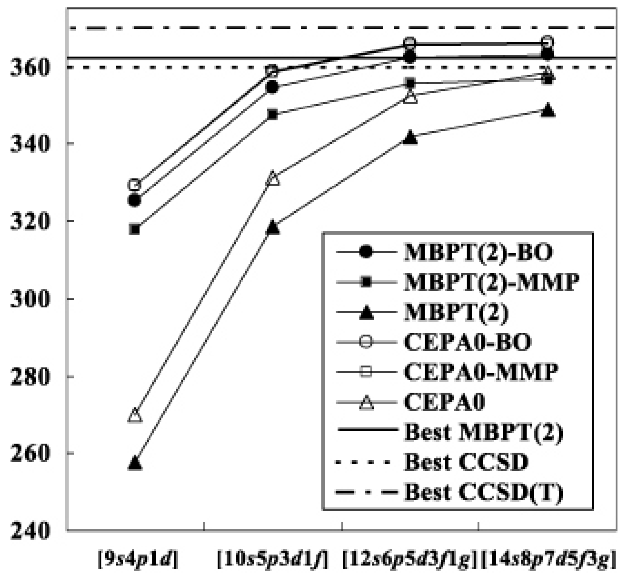
Table I shows the result for H2O. At the second order level, the results are relatively sensitive to the choice of the reference functions; the differences of the correlation energies are as large as between the modified MP and biorthogonal theories. However, they decrease as the order of perturbation increases. Finally the differences converge to the LCCSD values, ca. , with all of the basis sets. The basis set dependencies of the MBPT(2) and LCCSD energies are depicted in Fig. 2. For comparison, we show the R12-MBPT(2), CCSD and CCSD(T) energies for H2O with 374 basis functions [33]. The difference between the conventional and transcorrelated LCCSD energies is with the set. This means that the use of the present methods are particularly advantageous with such a small basis set. The energies of the transcorrelated methods seem almost
![Ijms 03 00459 g002]() saturated in each order with the set, while the conventional methods still gain the correlation energies of from to set. The absolute correlation energies of the transcorrelated LCCSD methods with the largest set are as low as that of R12-CCSD. The usual situation that the fourth order quadruples diagrams contribute positive [34] holds in the transcorrelated methods.
saturated in each order with the set, while the conventional methods still gain the correlation energies of from to set. The absolute correlation energies of the transcorrelated LCCSD methods with the largest set are as low as that of R12-CCSD. The usual situation that the fourth order quadruples diagrams contribute positive [34] holds in the transcorrelated methods.

| Basis Set | Orderb) | Modified MP | Biorthogonal | Conventional |
|---|---|---|---|---|
| 2nd | 325.38 | 317.76 | 257.74 | |
| 3rd | 323.40 | 322.82 | 263.61 | |
| 4th | 328.08 | 327.38 | 268.58 | |
| 329.34 | 329.02 | 270.20 | ||
| 2nd | 354.54 | 347.34 | 318.46 | |
| 3rd | 352.19 | 351.37 | 323.38 | |
| 4th | 357.78 | 356.97 | 329.65 | |
| 358.95 | 358.53 | 331.14 | ||
| 2nd | 362.20 | 355.47 | 341.90 | |
| 3rd | 358.86 | 357.89 | 344.43 | |
| 4th | 364.70 | 363.89 | 351.14 | |
| 365.85 | 365.38 | 352.55 | ||
| 2nd | 363.11 | 356.54 | 348.89 | |
| 3rd | 359.24 | 358.17 | 350.14 | |
| 4th | 365.18 | 364.38 | 357.11 | |
| 366.34 | 365.87 | 358.50 |
a) In -mEh unit.
b) Order of the perturbation in the correlation energy within LCCSD.
c) Nearly exact correlation energies are -361.486, -359.775 and -369.89 mEh at the R12-MBPT(2)-A, R12-CCSD and R12-CCSD(T) levels of approximations with 374 Gaussian-type functions.
Figure 2.
Convergence of the correlation energy of H2O. The abbreviated notations, BO and MMP, denote the biorthogonal and modified MP methods, respectively.
Figure 2.
Convergence of the correlation energy of H2O. The abbreviated notations, BO and MMP, denote the biorthogonal and modified MP methods, respectively.

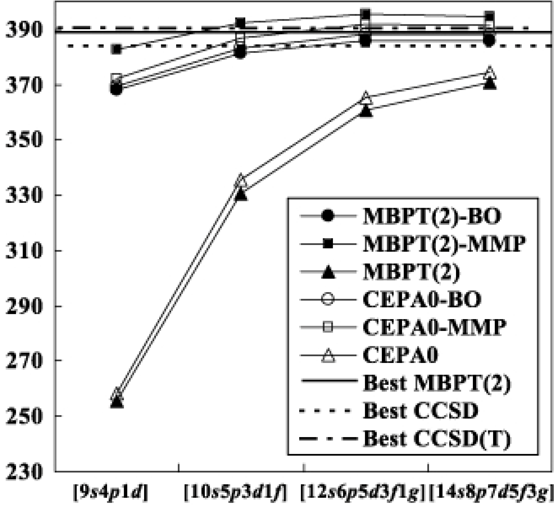
Let us proceed to the result of Ne in Table II. In comparison with the H2O result, the differences between the modified MP and biorthogonal methods are larger by the amounts, ca. and at the MBPT(2) and LCCSD levels, respectively. Especially, the modifies MP series tends to overshoot the correlation energy for the system. The method is considered to become less adequate for Ne because of the increasing magnitude of especially for the description of correlations including core electrons. The inclusions of higher-order corrections will be required to recover the difference. The convergence behaviors are shown in Fig. 3. In spite of the increase of the discrepancy between the two biorthogonal methods, the basis set dependence is similar to that for H2O beyond the set; the differences are sufficiently small within between the to sets. With the small sets, and , the transcorrelated method of the biorthogonal reference reproduces 95.4% and 98.8% of the saturated energies at the second order
![Ijms 03 00459 g003]() level, while the conventional method covers only 65.8% and 85.1% of the R12-MBPT(2)-A energy. Although the modified MP series slightly overshoots the correlation energies, the almost saturated biorthogonal LCCSD energy is in between the R12-CCSD and R12-CCSD(T) ones consistently with the previous results for H2O.
level, while the conventional method covers only 65.8% and 85.1% of the R12-MBPT(2)-A energy. Although the modified MP series slightly overshoots the correlation energies, the almost saturated biorthogonal LCCSD energy is in between the R12-CCSD and R12-CCSD(T) ones consistently with the previous results for H2O.
| Basis Set | Order b) | Modified MP | Biorthogonal | Conventional |
|---|---|---|---|---|
| 2nd | 382.54 | 368.19 | 255.48 | |
| 3rd | 371.75 | 366.67 | 255.97 | |
| 4th | 371.73 | 368.91 | 258.20 | |
| 372.19 | 369.20 | 258.56 | ||
| 2nd | 392.39 | 381.17 | 330.53 | |
| 3rd | 386.18 | 379.36 | 331.79 | |
| 4th | 386.16 | 383.06 | 335.18 | |
| 386.60 | 383.23 | 335.54 | ||
| 2nd | 395.40 | 385.93 | 360.63 | |
| 3rd | 391.21 | 383.65 | 361.12 | |
| 4th | 391.28 | 388.09 | 364.93 | |
| 391.72 | 388.15 | 365.27 | ||
| 2nd | 394.62 | 385.94 | 370.69 | |
| 3rd | 391.00 | 383.08 | 370.13 | |
| 4th | 391.09 | 387.91 | 374.13 | |
| 391.52 | 387.89 | 374.46 |
a) In -mEh unit.
b) Order of the perturbation in the correlation energy within LCCSD.
c) Nearly exact correlation energies are -388.311, -383.823 and -390.508 mEh at the R12-MBPT(2)-A, R12-CCSD and R12-CCSD(T) levels of approximations with 293 Gaussian-type functions.
Figure 3.
Convergence of the correlation energy of Ne. The notations are same as those in Figure 2.
Figure 3.
Convergence of the correlation energy of Ne. The notations are same as those in Figure 2.

We show the results of the entire 10-electronic systems with the set in Table III. The biorthogonal SCF and pseudo orbital energies, and , differ from each other by increasingly with the mass of the main elements. This is relevant to the descriptions concerning 1s core electrons as mentioned previously. The differences, however, reduce to at the LCCSD levels. The biorthogonal LCCSD results are always in the range between R12-CCSD and R12-CCSD(T). Especially the energies are consistently below the R12-CCSD energies by , implying that the results are reliable in the basis set convergence. For further improvements of the absolute energies, inclusion of the primary fourth order diagrams of triple- and quadruple-excitations will be necessary.
6. CONCLUSION
We have seen that the use of the transcorrelated Hamiltonian is particularly effective for accelerating the convergence of correlation energies with the size of one electronic basis. The key features of the method are in the following. We employ the symmetric correlation factor, which is commutable with the Coulomb potential. This leads to the simple structure of the transcorrelated Hamiltonian. The explicitly correlated functions are used to deal with the short-range behavior of the many-electron wave functions. Instead, the residual correlation effects, which are long-ranged, are treated in terms of the usual CI-type expansion with one-electronic basis. Thus the number of the additional integrals
grows linearly to the system size, making the application to large molecular systems feasible. The short-range nature of the correlation factor is also effective to make the three-body contributions less important. This property allows us to use the resolution of identity appropriately for the quantities less significant than the ones like , which appear in other theories. As a result, the original scaling of a correlated method is maintained even after the introduction of the transcorrelated Hamiltonian.
Table III.
Correlation energies of Ne, HF, H2O, NH3 and CH4 molecules with the [12s6p5d3f1g/5s3p2d1f] basis seta)
| Ne | HF | H2O | NH3 | CH4 | |
|---|---|---|---|---|---|
| HF | 128543.47 | 100067.71 | 76064.89 | 56223.14 | 40216.34 |
| Conv. MBPT(2) | 360.63 | 360.58 | 341.90 | 307.07 | 260.33 |
| Conv. LCCSD | 365.27 | 366.36 | 352.55 | 325.52 | 287.61 |
| Biorthogonal | |||||
| SCF | 184.14 | 138.06 | 102.13 | 74.70 | 53.77 |
| 2nd order | 385.93 | 379.11 | 355.47 | 316.74 | 267.71 |
| 3rd order | 383.65 | 376.99 | 357.89 | 326.77 | 285.68 |
| 4th order | 388.09 | 382.95 | 363.89 | 332.56 | 291.82 |
| LCCSD | 388.15 | 383.63 | 365.38 | 334.62 | 294.39 |
| Modified MP | |||||
| Pseudo Orbital | 222.47 | 158.84 | 112.55 | 79.55 | 55.84 |
| 2nd order | 395.40 | 387.80 | 362.20 | 321.14 | 270.03 |
| 3rd order | 391.21 | 381.04 | 358.86 | 326.33 | 285.11 |
| 4th order | 391.28 | 384.66 | 364.70 | 332.80 | 291.70 |
| LCCSD | 391.72 | 385.47 | 365.85 | 334.41 | 294.02 |
| R12b) | |||||
| MBPT(2)-A | 387.910 | 384.357 | 361.691 | 322.400 | 273.579 |
| CCSD | 382.945 | 378.392 | 359.312 | 327.829 | 288.557 |
| CCSD(T) | 389.456 | 387.260 | 369.228 | 337.248 | 295.948 |
a) In -mEh unit. b) The correlation energies with basis set.
There are mass dependences of the reference energies of the transcorrelated Hamiltonian, and , because the operator, , brings more significant contribution on the core electrons as the atomic mass increases. The correlation behaviors are different between the core and valence shells. The original transcorrelated method as well as most of the GTG methods use explicitly correlated functions, which are dependent on the positions of electrons. The introduction of such position dependence will enable more balanced treatment of different shells though the evaluation of integrals becomes complicated. The use of the spherically symmetric geminal is much more feasible. The present result implies that the ignorance of the position dependence does not spoil the accuracy at the LCCSD level to say the least for elements as heavy as Ne.
For calculations of excited states and bond breakings, multireference treatment is necessary. Such an application of the transcorrelated Hamiltonian is also straightforward. Extensions in this line are now under progress. Another application will be the calculation of static structure factors [35,36]. Since this quantity is a probe sensitive to the dynamic correlation effects, comparisons with experimental data will be an important measure of the explicitly correlated method.
Acknowledgement
The present work is partly supported by the Grant-in-Aids for Scientific Research on Priority Areas (A) (No. 12042233) from the Ministry of Education, Culture, Sports, Science and Technology in Japan, and for Scientific Research (B) (No. 13440177) from the Japan Society for the Promotion of Science.
References
- Kato, T. Commun. Pure Appl. Math. 1957, 10, 151. [CrossRef]
- Boys, S. F. Proc. Roy. Soc. London Ser. 1960, A258, 402. [CrossRef]
- Singer, K. Proc. Roy. Soc. London Ser. 1960, A258, 412. [CrossRef]
- Szalewicz, K.; Jeziorski, B.; Monkhorst, H. J.; Zabolitzky, J. G. J. Chem. Phys. 1983, 78, 1420.
- Szalewicz, K.; Zabolitzky, J. G.; Jeziorski, B.; Monkhorst, H. J. J. Chem. Phys. 1984, 81, 2723.
- Cencek, W.; Rychlewski, J. J. Chem. Phys. 1993, 98, 1252.
- Bukowski, R.; Jeziorski, B.; Szalewicz, K. J. Chem. Phys. 1999, 110, 4165.
- Cencek, W.; Rychelewski, J. Chem. Phys. Lett. 2000, 320, 549.
- Kutzelnigg, W. Theor. Chim. Acta. 1985, 68, 445. [CrossRef]
- Kutzelnigg, W.; Klopper, W. J. Chem. Phys. 1991, 94, 1985.
- Termath, V.; Klopper, W.; Kutzelnigg, W. J. Chem. Phys. 1991, 94, 2002.
- Klopper, W.; Kutzelnigg, W. J. Chem. Phys. 1991, 94, 2020.
- Noga, J.; Kutzelnigg, W. J. Chem. Phys. 1994, 101, 7738.
- Noga, J.; Tunega, D.; Klopper, W.; Kutzelnigg, W. J. Chem. Phys. 1995, 103, 309.
- Noga, J.; Klopper, W.; Kutzelnigg, W. Recent Advances in Coupled-Cluster Methods; Bartlett, R.J., Ed.; World Scientific, 1997. [Google Scholar]
- Persson, B. J.; Taylor, P.R. J. Chem. Phys. 1996, 105, 5915.
- Boys, S. F.; Handy, N. C. Proc. R. Soc. 1969, A 310, 43. [CrossRef]
- Handy, N. C. Mol. Phys. 1973, 26, 169.
- Ten-no, S. Chem. Phys. Lett. 2000, 330, 169.
- Ten-no, S. Chem. Phys. Lett. 2000, 330, 175.
- Hino, O.; Tanimura, Y.; Ten-no, S. J. Chem. Phys. 2001, 115, 7865.
- Obara, S.; Saika, A. J. Chem. Phys. 1988, 89, 1540.
- Dupuis, M.; Rys, J.; King, H. F. J. Chem. Phys. 1976, 65, 111.
- Dupuis, M.; Marquez, A. J. Chem. Phys. 2001, 114, 2067.
- Meyer, W. J. Chem. Phys. 1973, 58, 1017.
- Kutzelnigg, W. Method of Electronic Structure Theory; Shaefer, H.F., Ed.; Plenum: New York, 1977; p. 129. [Google Scholar]
- Koch, H.; Christiansen, O.; Kobayashi, R.; Jørgensen, P.; Helgaker, T. Chem. Phys. Lett. 1994, 228, 233.
- Ten-no, S.; Iwata, S.; Pal, S.; Mukherjee, D. Theor. Chem. Acc. 1999, 102, 252. [CrossRef]
- Mayer, I. Int. J. Quantum Chem. 1983, 23, 341. [CrossRef]
- Surján, P. R.; Mayer, I.; Lukovits, I. Chem. Phys. Lett. 1985, 119, 538.
- Dunning, T. H., Jr. J. Chem. Phys. 1989, 90, 1007.
- Woon, D. E.; Dunning, T. H., Jr. J. Chem. Phys. 1995, 103, 4572.
- Helgaker, T.; Klopper, W.; Koch, H.; Noga, J. J. Chem. Phys. 1997, 106, 9639.
- Bartlett, R. J. Ann. Rev. Phys. Chem. 1981, 32, 359. [CrossRef]
- Watanabe, N.; Hayashi, H.; Udagawa, Y.; Ten-no, S.; Iwata, S. J. Chem. Phys. 1998, 108, 4545.
- Watanabe, N.; Ten-no, S.; Pal, S.; Iwata, S.; Udagawa, Y. J. Chem. Phys. 1999, 111, 827.
© 2002 by MDPI (http://www.mdpi.org).
Share and Cite
MDPI and ACS Style
Ten-no, S.; Hino, O. New Transcorrelated Method Improving the Feasibility of Explicitly Correlated Calculations. Int. J. Mol. Sci. 2002, 3, 459-474. https://doi.org/10.3390/i3050459
AMA Style
Ten-no S, Hino O. New Transcorrelated Method Improving the Feasibility of Explicitly Correlated Calculations. International Journal of Molecular Sciences. 2002; 3(5):459-474. https://doi.org/10.3390/i3050459
Chicago/Turabian StyleTen-no, Seiichiro, and Osamu Hino. 2002. "New Transcorrelated Method Improving the Feasibility of Explicitly Correlated Calculations" International Journal of Molecular Sciences 3, no. 5: 459-474. https://doi.org/10.3390/i3050459