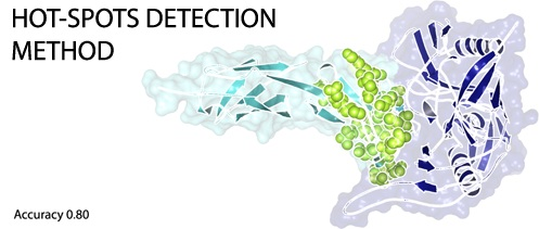
A Machine Learning Approach for Hot-Spot Detection at Protein-Protein Interfaces

Abstract

Understanding protein-protein interactions is a key challenge in biochemistry. In this work, we describe a more accurate methodology to predict Hot-Spots (HS) in protein-protein interfaces from their native complex structure compared to previous published Machine Learning (ML) techniques. Our model is trained on a large number of complexes and on a significantly larger number of different structural- and evolutionary sequence-based features. In particular, we added interface size, type of interaction between residues at the interface of the complex, number of different types of residues at the interface and the Position-Specific Scoring Matrix (PSSM), for a total of 79 features. We used twenty-seven algorithms from a simple linear-based function to support-vector machine models with different cost functions. The best model was achieved by the use of the conditional inference random forest (c-forest) algorithm with a dataset pre-processed by the normalization of features and with up-sampling of the minor class. The method has an overall accuracy of 0.80, an F1-score of 0.73, a sensitivity of 0.76 and a specificity of 0.82 for the independent test set.

1. Introduction

Among all of the cellular components of living systems, proteins are the most abundant and the most functionally versatile. The specific interactions formed by these macromolecules are vital in a wide-range of biological pathways [1]. Protein-protein interactions involved in both transient and long-lasting networks of specific complexes play important roles in many biological processes [2,3,4]. Characterizing the critical residues involved in these interactions by both experimental and computational methods is therefore crucial to a proper understanding of living systems. Furthermore, only by gaining a complete understanding at atomistic detail can new methods be developed to modulate their binding [5,6].

Protein-protein interfaces often involve a large number of residues. However, it is generally recognized that small regions of a few residues, termed “Hot-Spots (HS)”, are essential for maintaining the integrity of the interface. The development of techniques to identify and characterize protein-based interfaces has become widespread. Experimental Alanine Scanning Mutagenesis (ASM) continues to be a valuable technique for both detecting and analyzing protein-binding interfaces. The contribution of a residue to the binding energy is measured by the binding free energy difference (ΔΔG_binding) between the wild-type (WT) and mutant complex upon mutation of a specific residue to alanine [7]. Bogan and Thorn [8] defined the residues with ΔΔG_binding ≥ 2.0 kcal·mol⁻¹ as HS; and the residues with ΔΔG_binding < 2.0 kcal·mol⁻¹ as Null-Spots (NS). Experimental methods for identifying HS are based on molecular biology techniques that are accurate, but still complex, time-consuming and expensive [9]. Highly efficient computational methods for predicting HS can provide a viable alternative to experiments. Molecular Dynamics (MD) simulations can be used to predict changes in the binding strength of protein complexes by calculating the free energy difference from an initial to a final state [10,11]. However, due to the complexity and typical large size of protein-protein complexes, these methods are still computationally expensive. Recently, machine learning approaches trained on various features of experimentally-determined HS residues have been developed in order to predict HS in new protein complexes [6,12,13,14].

In previous work, we have investigated feature-based methods combining Solvent Accessible Surface Area (SASA) descriptors calculated from static structures and MD ensembles and trained predictors using a Support Vector Machine (SVM) algorithm [15]. However, we only applied these to a small number of complexes, and the prediction performance was hampered by a high number of false positives. More recently, we added an extra feature (residue evolutionary sequence conservation) on a significantly larger dataset. In that study, we explored additional Machine Learning (ML) techniques, which led us to develop a more accurate and time-efficient HS detection methodology. This resulted in new HS predictor models for both protein-protein and protein-nucleic acid interactions, and we implemented the best performing models into two web tools [14].

In this study, we significantly expand both the number of studied protein-protein complexes and the number of 3D complex structure-based features used for prediction, including: interface size, the type of interaction between residues at the interface of the complex and the number of different types of residues at the interface. To the evolutionary sequence-based features, we added the Position-Specific Scoring Matrix (PSSM), for a total of 79 features. We have further tested a total of 27 algorithms from a simple linear-based function to support-vector machine models with different cost functions. The best predictor, based on a conditional inference random forest (c-forest) algorithm, achieves an overall performance characterized with an F1-score of 0.73, an accuracy of 0.80, a sensitivity of 0.76 and a specificity of 0.82. To the best of our knowledge, these values are higher than all other available prediction techniques.

2. Results

In the current study, we have used the Classification And Regression Training (Caret) Package [16] from the R software [17], which provides a unified interface with a large number of built-in classifiers, in order to train an HS predictor. The dataset used for this purpose includes 545 amino acids from 53 complexes (140 HS and 405 NS). We calculated the percentage of the different types of amino acids within the NS set (Ser: 7.4; Gly: 1.5; Pro: 2.0; Val: 3.2; Leu: 2.7; Ile: 5.2; Met: 1.0; Cys: 0.7; Phe: 4.7; Tyr: 5.9; Trp: 4.9; His: 4.4; Lys 8.9; Arg: 10.6; Gln: 5.4; Asn: 6.2; Glu: 9.9; Asp: 7.2; Thr: 8.1) and within the HS set (Ser: 2.1; Gly: 2.9; Pro: 2.9; Val: 3.6; Leu: 7.1; Ile: 4.3; Met: 0.0; Cys: 0.0; Phe: 6.4; Tyr: 20.0; Trp: 5.7; His: 2.1; Lys 7.1; Arg: 6.4; Gln: 2.1; Asn: 5.0; Glu: 7.1; Asp: 10.7; Thr: 4.3). For both sets, there is a natural expected tendency for a higher percentage of large hydrophobic or charged residues at the interfaces, in particular Tyr. Although different patterns could influence the training of a robust classifier, we have previously successfully constructed models that were bias-free for all different amino acids [14]. We randomly split this dataset (see for details Supplementary Information Table S1) into a training set consisting of 70% of data (382 mutations) and an independent test set (163 mutations, 30%). This is a standard division scheme demonstrated to give a good result. All 27 classification models (listed in the Methods Section) were tested using 10-fold cross-validation repeated 10 times in order to avoid overfitting and to obtain the model’s generalization error. This means that the training set was split randomly into ten isolated parts, using nine of the ten parts to train the model and taking the remaining fold of data to test the final performance of the model. This process was repeated ten times. The performance of the five best algorithms for each tested condition was independently evaluated on the test set to ensure an unbiased assessment of the accuracy of the final model.

The 79 features used in this work have different scales (i.e., the range of the raw data varies significantly), and therefore, we have performed feature normalization or data standardization of the predictor variables at the training set by centering the data, i.e., subtracting the mean and normalizing it by dividing by the standard deviation. The same protocol was followed for the test set taking into account the use of the training mean and standard deviation to ensure a good estimation of the model quality and generalization power. As we have a high-dimensional dataset (79 features), we have also applied Principal Components Analysis (PCA) to reduce the dimensionality of the data. PCA works by establishing an orthogonal transformation of the data to convert a set of possible correlated variables into a set of linearly-uncorrelated ones, the so-called principal components.

One of the main concerns when applying classification to the detection of HS is the natural imbalance of the data. As expected, the number of HS is lower than the number of NS at a protein-protein interface, as indicated by the presence of 185 HS and 360 NS in the main dataset. In ML classification methods, the disparity of the frequencies of the observed classes may have a very negative impact on the models’ performance. To overcome this problem, we have tried two different subsampling techniques for the training set: down-sampling and up-sampling. In the first, there is a random sub-setting of all classes at the training set with their class frequency matching the least prevalence class (HS), whereas in the up-sampling, the opposite is happening with random sampling (with the replacement) of the minority class (HS) to reach the same size as the majority class (NS). Different conditions were thus established: (i) Scaled; (ii) Scaled Up; (iii) Scaled Down; (iv) PCA; (v) PCA Down; and (vi) PCA Up. Various statistical metrics (described in detail in the Methods Section) were adopted to evaluate the performance of the algorithms tested: Area Under the Receiver Operator Curve (AUROC), accuracy, True Positive Rate (TPR), True Negative Rate (TNR), Positive Predictive Value (PPV), False Positive Rate (FPR), False Negative Rate (FNR) and F1-score. Figure 1 illustrates the workflow followed in this study.

The results for the training set for the best five algorithms for each of the six conditions studied are listed in

Table 1. Statistical metrics attained for five algorithms with top performance for each of the studied conditions for the training set.

Pre-Processing	Metrics	Algorithms
Scaled		Nnet	avNNET	C5.0 Tree	C5.0 Rules	svmRadialSigma
	AUROC	0.52	0.65	0.77	0.72	0.78
	Accuracy	0.92	0.94	0.96	0.92	0.91
	Sensitivity	0.92	0.88	0.88	0.85	0.80
	Specificity	0.91	0.98	1.00	0.96	0.97
	PPV	0.86	0.95	0.99	0.92	0.93
	NPV	0.95	0.94	0.94	0.92	0.89
	FPR	0.09	0.02	0.00	0.04	0.03
	F1-score	0.89	0.92	0.93	0.89	0.86
Scaled_Down		c-Forest	avNNET	C5.0Tree	C5.0Rules	GBM
	AUROC	0.79	0.70	0.73	0.71	0.80
	Accuracy	0.91	0.95	0.96	0.90	1.00
	Sensitivity	0.93	0.96	0.96	0.89	0.99
	Specificity	0.90	0.93	0.95	0.91	1.00
	PPV	0.90	0.93	0.95	0.9	1.00
	NPV	0.92	0.96	0.96	0.89	0.99
	FPR	0.1	0.07	0.05	0.09	0
	F1-score	0.91	0.95	0.96	0.9	1.00
Scaled_Up		c-Forest	avNNET	C5.0Tree	C5.0Rules	GBM
	AUROC	0.85	0.75	0.85	0.82	0.84
	Accuracy	0.93	0.94	0.98	0.95	0.98
	Sensitivity	0.93	0.96	0.99	0.96	0.97
	Specificity	0.93	0.92	0.97	0.94	0.99
	PPV	0.93	0.92	0.97	0.94	0.99
	NPV	0.93	0.96	0.99	0.95	0.97
	FPR	0.07	0.08	0.03	0.06	0.01
	F1-score	0.93	0.94	0.98	0.95	0.98
PCA		nnet	avNNET	C5.0Tree	C5.0Rules	svmRadialSigma
	AUROC	0.69	0.75	0.61	0.59	0.76
	Accuracy	1.00	0.99	0.98	0.92	0.91
	Sensitivity	1.00	0.97	0.98	0.91	0.76
	Specificity	1.00	1.00	0.98	0.93	0.99
	PPV	1.00	0.99	0.96	0.89	0.97
	NPV	1.00	0.98	0.99	0.95	0.88
	FPR	0	0	0.02	0.07	0.01
	F1-score	1.00	0.98	0.97	0.90	0.85
PCA_Down		nnet	avNNET	C5.0Tree	C5.0Rules	svmRadialSigma
	AUROC	0.70	0.78	0.67	0.67	0.75
	Accuracy	0.87	0.91	0.97	0.91	0.91
	Sensitivity	0.88	0.88	0.96	0.96	0.88
	Specificity	0.87	0.93	0.99	0.87	0.93
	PPV	0.87	0.92	0.99	0.88	0.93
	NPV	0.88	0.89	0.96	0.95	0.89
	FPR	0.13	0.07	0.01	0.13	0.07
	F1-score	0.87	0.90	0.97	0.92	0.91
PCA_Up		nnet	avNNET	C5.0Tree	C5.0Rules	svmRadialSigma
	AUROC	0.75	0.82	0.80	0.78	0.80
	Accuracy	0.95	0.98	0.98	0.96	0.94
	Sensitivity	0.94	0.97	0.99	0.96	0.92
	Specificity	0.96	0.99	0.98	0.96	0.95
	PPV	0.96	0.99	0.98	0.96	0.95
	NPV	0.94	0.97	0.99	0.96	0.92
	FPR	0.04	0.01	0.02	0.04	0.05
	F1-score	0.95	0.98	0.98	0.96	0.94

avNNET: model averaged Neural Network; C5.0 Rules (single C5.0 Ruleset); C5.0 Tree (single C5.0 Tree); c-forest (conditional inference random forest); GBM (stochastic gradient boosting machine); nnet (neuronal network); svmRadialSigma (support vector machines with the Radial basis function kernel); Positive Predictive Value (PPV); Negative Predictive Value (NPV); False Positive Rate (FPR).

. All statistical metrics obtained for the complete set of algorithms can be found in Supplementary Information Table S2, in which a more straightforward comparison by type of method can be made. The best classifiers seem to be almost constant in all six different pre-processing conditions, including one neuronal network (avNNET: model averaged Neural Network) and two tree-based methods (C5.0 Tree, C5.0 Rules). The fourth and fifth classifiers vary from nnet (neuronal network), to c-forest, GBM (stochastic gradient boosting machine) and svmRadialSigma (support vector machines with the Radial basis function kernel). The up-sampling of the HS class seems to improve the classifier performance presenting AUROC values higher than 0.80 in the majority of the cases.

The performance of a classifier on the training set from which it was constructed gives a poor estimate of its accuracy in new cases. Furthermore, overfitting on algorithms without regularization terms (such as decision trees and neural networks) is harder to address on the training set. Therefore, the true predictive accuracy of the classifier was estimated on a separate test set corresponding to 30% of the main dataset.

Table 2. Statistical metrics attained for 5 algorithms with the top performance for each of the studied conditions for the independent test set.

Pre-Processing	Metrics	Algorithms
Scaled		Nnet	avNNET	C5.0 Tree	C5.0 Rules	svmRadialSigma
	AUROC	0.71	0.68	0.68	0.72	0.70
	Accuracy	0.74	0.71	0.71	0.74	0.73
	Sensitivity	0.57	0.57	0.5	0.60	0.55
	Specificity	0.83	0.79	0.83	0.82	0.83
	PPV	0.65	0.6	0.62	0.65	0.64
	NPV	0.78	0.77	0.75	0.79	0.77
	FPR	0.43	0.43	0.4	0.4	0.45
	F1-score	0.61	0.58	0.55	0.62	0.59
Scaled_Down		c-forest	avNNET	C5.0 Tree	C5.0 Rules	GBM
	AUROC	0.75	0.68	0.63	0.71	0.73
	Accuracy	0.76	0.69	0.64	0.72	0.75
	Sensitivity	0.79	0.71	0.67	0.76	0.74
	Specificity	0.74	0.69	0.62	0.70	0.75
	PPV	0.63	0.55	0.49	0.59	0.62
	NPV	0.87	0.81	0.77	0.84	0.84
	FPR	0.21	0.29	0.33	0.24	0.26
	F1-score	0.7	0.62	0.57	0.66	0.68
Scaled_Up		c-forest	AvNNET	C5.0 Tree	C5.0 Rules	GBM
	AUROC	0.78	0.73	0.65	0.70	0.80
	Accuracy	0.80	0.75	0.69	0.73	0.82
	Sensitivity	0.76	0.66	0.48	0.59	0.76
	Specificity	0.82	0.80	0.80	0.81	0.85
	PPV	0.70	0.64	0.57	0.63	0.73
	NPV	0.86	0.81	0.74	0.78	0.86
	FPR	0.24	0.34	0.52	0.41	0.24
	F1-score	0.73	0.65	0.52	0.61	0.75
PCA		Nnet	avNNET	C5.0 Tree	C5.0 Rules	svmRadialSigma
	AUROC	0.65	0.73	0.68	0.71	0.71
	Accuracy	0.67	0.75	0.7	0.74	0.74
	Sensitivity	0.60	0.60	0.66	0.67	0.52
	Specificity	0.71	0.84	0.72	0.77	0.86
	PPV	0.54	0.67	0.57	0.62	0.67
	NPV	0.77	0.79	0.79	0.81	0.76
	FPR	0.4	0.4	0.34	0.33	0.48
	F1-score	0.57	0.64	0.61	0.64	0.58
PCA_Down		Nnet	avNNET	C5.0 Tree	C5.0 Rules	svmRadialSigma
	AUROC	0.70	0.68	0.59	0.61	0.69
	Accuracy	0.71	0.69	0.61	0.63	0.70
	Sensitivity	0.76	0.71	0.55	0.60	0.72
	Specificity	0.68	0.69	0.64	0.64	0.69
	PPV	0.56	0.55	0.46	0.48	0.56
	NPV	0.84	0.81	0.72	0.74	0.82
	FPR	0.24	0.29	0.45	0.4	0.28
	F1-score	0.65	0.62	0.50	0.53	0.63
PCA_Up		Nnet	avNNET	C5.0 Tree	C5.0 Rules	svmRadialSigma
	AUROC	0.67	0.75	0.56	0.61	0.69
	Accuracy	0.7	0.77	0.59	0.63	0.71
	Sensitivity	0.59	0.64	0.48	0.55	0.64
	Specificity	0.76	0.84	0.65	0.68	0.75
	PPV	0.58	0.69	0.43	0.48	0.59
	NPV	0.77	0.81	0.69	0.73	0.79
	FPR	0.41	0.36	0.52	0.45	0.36
	F1-score	0.58	0.66	0.46	0.52	0.61

avNNet: model averaged Neural Network; C5.0 Rules (single C5.0 Ruleset); C5.0 Tree (single C5.0 Tree); c-forest (conditional inference random forest); GBM (stochastic gradient boosting machine); nnet (neuronal network); svmRadialSigma (support vector machines with the Radial basis function kernel).

summarizes the performance on the independent test set for the best classifiers shown in Table 1.

From all of methods, c-forest, trained on the normalized up-scaling set, had the highest performance metrics on both training and test sets. It was therefore chosen as a final model. In our analysis of this classifier (Figure 2), we observed that the key features are structural ones: specifically, relSASA_i, ΔSASA_i, the number of contacts established by the interfacial residues at 4 Å and the number of LEU, VAL and HIS residues at the interface. All of these features were calculated using built-in functions of the VMD package [18] and in-house scripts.

To validate the accuracy of the best predictor, we performed the HS predictions with other methods reported in the literature, such as Robetta [19], KFC2-A (Knowledge-based FADE and Contacts) [20], KFC2-B [20] and CPORT (Consensus Prediction Of interface Residues in Transient complexes)(not specialized in HS prediction, but instead, a protein-protein interface predictor) [21] on the same training and test sets. The comparison among these ML methods (

Table 3. Comparison of the statistical metrics attained for the best predictor in this work and some of the most common ones in the literature.

Perfomance	Algorithms
	c-Forest/ Up-Scaling Classes		SBHD2		Robetta		KFC2-A		KFC2-B		CPORT
	Training	Test	Training	Test	Training	Test	Training	Test	Training	Test	Training	Test
AUROC	0.85	0.78	0.74	0.69	0.62	0.62	0.72	0.66	0.60	0.67	0.54	0.54
Accuracy	0.93	0.80	0.70	0.71	0.66	0.66	0.76	0.71	0.70	0.73	0.49	0.49
Sensitivity	0.93	0.76	0.70	0.70	0.38	0.29	0.57	0.53	0.26	0.28	0.55	0.54
Specificity	0.93	0.82	0.70	0.71	0.85	0.88	0.85	0.81	0.93	0.96	0.45	0.47
PPV	0.93	0.70	0.55	0.56	0.61	0.60	0.67	0.59	0.65	0.80	0.34	0.35
NPV	0.93	0.86	0.82	0.82	0.68	0.67	0.79	0.77	0.71	0.72	0.66	0.66
F1-score	0.93	0.73	0.62	0.62	0.47	0.39	0.62	0.56	0.37	0.42	0.42	0.42

) demonstrates that our new method achieves the best performance with F1-scores/AUROC values of 0.73/0.78 on the test set against 0.39/0.62, 0.56/0.66, 0.42/0.67 and 0.43/0.54 for Robetta, KFC2-A, KFC2-B and CPORT, respectively.

3. Discussion

Machine learning is an area of artificial intelligence that is data driven with a focus on the development of computational techniques for making inferences or predictions. It has become widely used in a variety of areas due to its reduced application time and high performance. Over the past few years, a few algorithms have been applied for the specific problem in this study: the detection of hot-spots at protein-protein interfaces [13,14,15,22,23,24,25,26,27,28,29,30,31,32,33,34,35].

Here, neural networks and tree-based methods were highlighted as some of the high performance classifiers. Neural networks are inspired by biological nervous systems transmitting the information by a vast network of interconnecting processing elements (neurons). Decision trees organize the knowledge extracted from a hierarchy by using simple tests over the features of the training set. Both have been shown in the past to be promising ML algorithms in the bioinformatics field. Random forests were also shown to be able to predict the impact of each variable in high dimensional problems even in the presence of complex interactions [36]. In particular, c-forest [36], an implementation of the random forest and bagging ensemble method that uses conditional inference trees as base learners, achieved the top performance (Table 2) with a high F1-score of 0.93 on the training set using a 10 repeated 10-fold cross-validation. The values in the independent test (F1 score 0f 0.73) were also very high compared to the ones currently reported in the literature and surpassing all of the other methods tested in this study (Table 3; SBHD (Sasa-Based Hot-spot Detection) 0.61, Robetta 0.39, KFC2-A 0.56, KFC2-B 0.42 and CPORT 0.42). One important aspect that seemed to improve the results compared to our previous approaches (SBHD) was the use of in-built R techniques to balance the training data: up-scaling of the data led to a substantial improvement of the F1-score and to a decrease of the FPR to about 0.19 on the independent test set. In this particular classifier, the first seven features with higher importance were all structure-based: two already used in previous versions of our algorithm (ΔSASA_i and relSASA_i, check Material and Methods) and five new ones (the number of residues at a 4 Å distance and the number of LEU, VAL, HIS and PRO residues at the interface). The PSSM value for the TYR residues, one of the most common residues as HS, was the first genomic-based feature to be ranked as important.

4. Material and Methods

4.1. Dataset Construction

We constructed a database of complexes by combining information from the Alanine Scanning Energetics database (ASEdb) [37], the Binding Interface Database (BID) [38] and the SKEMPI (Structural database of Kinetics and Energetics of Mutant Protein Interactions) [39] and PINT (Protein-protein Interactions Thermodynamic Database) [40] databases, which provide both experimental ΔΔG_binding values for interfacial residues and tridimensional (3D) X-ray structure information. The protein sequences were filtered to ensure a maximum of 35% sequence identity for at least one protein in each interface. Crystal structures were retrieved from the Protein Data Bank (PDB) [41], and all water molecules, ions and other small ligands were removed. Our final dataset consists of 545 mutations from 53 different complexes.

4.2. Sequence/Structural Features

From a structural point of view, we compiled 12 previously-used different SASA descriptors for all interfacial residues [14,15]: (i) _compSASA_i, the solvent accessible surface area of residue i in the complex form; (ii) _monSASA_i, the residue SASA in the monomer form; (iii) ΔSASA_i, the SASA difference upon complexation (Equation (1)); (iv) relSASA_i, the ratio between ΔSASA for each residue and the _monSASA_i value for the same residue (Equation (2)). A further four features (_comp/resSASA_i, _mon/resSASA_i, _Δ/resSASA_i and _rel/resSASA_i), defined by Equations (3)–(6), were determined applying amino acid standardization by dividing the previous features by the average protein _resSASA_r values as determined by Miller and colleagues [42,43], with r being the respective residue type. Four additional, amino-acid standardized features were calculated by replacing the values determined by Miller by our own protein averages _aveSASA_r for each amino acid type in its respective protein: _comp/aveSASA_i, _mon/aveSASA_i, _Δ/aveSASA_i and _rel/aveSASA_i, defined in Equations (7)–(10).

$${\Delta \text{SASA}}_{\mathrm{i}}=\left|{}_{\text{comp}}{}^{}\mathrm{SASA}_{\mathrm{i}}^{}-{}_{\text{mon}}{}^{}\mathrm{SASA}_{\mathrm{i}}^{}\right|$$

(1)

$${}_{\text{rel}}{}^{}\mathrm{SASA}_{\mathrm{i}}^{}=\frac{{\Delta \text{SASA}}_{\mathrm{i}}}{{}_{\text{mon}}{}^{}\mathrm{SASA}_{\mathrm{i}}^{}}$$

(2)

$${}_{\text{comp}/\text{res}}{}^{}\mathrm{SASA}_{\mathrm{i}}^{}=\frac{{}_{\text{comp}}{}^{}\mathrm{SASA}_{\mathrm{i}}^{}}{{}_{\text{res}}{}^{}\mathrm{SASA}_{\mathrm{r}}^{}}$$

(3)

$${}_{\text{mon}/\text{res}}{}^{}\mathrm{SASA}_{\mathrm{i}}^{}=\frac{{}_{\text{mon}}{}^{}\mathrm{SASA}_{\mathrm{i}}^{}}{{}_{\text{res}}{}^{}\mathrm{SASA}_{\mathrm{r}}^{}}$$

(4)

$${}_{\Delta /\text{res}}{}^{}\mathrm{SASA}_{\mathrm{i}}^{}=\frac{{\Delta \text{SASA}}_{\mathrm{i}}}{{}_{\text{res}}{}^{}\mathrm{SASA}_{\mathrm{r}}^{}}$$

(5)

$${}_{\text{rel}/\text{res}}{}^{}\mathrm{SASA}_{\mathrm{i}}^{}=\frac{{\text{relSASA}}_{\mathrm{i}}}{{}_{\text{res}}{}^{}\mathrm{SASA}_{\mathrm{r}}^{}}$$

(6)

$${}_{\text{comp}/\text{ave}}{}^{}\mathrm{SASA}_{\mathrm{i}}^{}=\frac{{}_{\text{comp}}{}^{}\mathrm{SASA}_{\mathrm{i}}^{}}{{}_{\text{ave}}{}^{}\mathrm{SASA}_{\mathrm{r}}^{}}$$

(7)

$${}_{\text{mon}/\text{ave}}{}^{}\mathrm{SASA}_{\mathrm{i}}^{}=\frac{{}_{\text{mon}}{}^{}\mathrm{SASA}_{\mathrm{i}}^{}}{{}_{\text{ave}}{}^{}\mathrm{SASA}_{\mathrm{r}}^{}}$$

(8)

$${}_{\Delta /\text{ave}}{}^{}\mathrm{SASA}_{\mathrm{i}}^{}=\frac{{\Delta \text{SASA}}_{\mathrm{i}}}{{}_{\text{ave}}{}^{}\mathrm{SASA}_{\mathrm{r}}^{}}$$

(9)

$${}_{\text{rel}/\text{ave}}{}^{}\mathrm{SASA}_{\mathrm{i}}^{}=\frac{{\text{relSASA}}_{\mathrm{i}}}{{}_{\text{ave}}{}^{}\mathrm{SASA}_{\mathrm{r}}^{}}$$

(10)

As the SASA features described in Equations (3)–(10) are rather small, the results presented here were multiplied by a factor of 10³.

We further introduced two features directly related to the size of the interface: the total number of interfacial residues and the ΔSASA_total (sum of the ΔSASA_i of all residues at the protein-protein binding interfaces). Twenty other features were added by splitting the total number of interface residues into the 20 amino acid types. Four contact features were also calculated: (i) the number of protein-protein contacts within 2.5 Å and (ii) 4.0 Å distance cut-offs, respectively; (iii) the number of intermolecular hydrogen bonds; and (iv) the number of intermolecular hydrophobic interactions. In-house scripts using the VMD molecular package [18] were used for all of these calculations. We used in total 38 structural features in our study.

To utilize evolutionary sequence conservation information, we used the ConSurf server [44] that calculates a conservation score for each amino acid at an interfacial position for a complex, based on known sequences in different organisms. We also computed, PSSM using BLAST [45,46], as well as the weighted observed percentages, introducing them as 40 new features for all interfacial residues. Positive values in this matrix appear for substitutions more frequent than expected by random chance, and negative values indicate that the substitution is not frequent. Therefore, a total of 41 evolutionary sequence-related features were added to the structural features, resulting in 79 features in total for this study.

4.3. Machine Learning Techniques

We first pre-processed the dataset by eliminating missing values or NZV (Near Zero Variance) features. Next, as mentioned in the Results section, we normalized the dataset and performed PCA. The algorithms tested were: avNNet (model averaged Neural Network); bagEarth (bagged MARS (multivariate adaptive regression splines)); bagEarthGCV Bagged MARS using gCV pruning; bagFDA (bagged Flexible Discriminant Analysis); C5.0Rules (single C5.0 Ruleset); C5.0Tree (single C5.0 Tree); c-forest (conditional inference random forest); ctree (conditional inference tree); ctree2 (conditional inference tree); earth (multivariate adaptive regression spline); fda (flexible discriminant analysis); gaussprLinear (Gaussian process); GBM (stochastic gradient boosting machine); gcvEarth (multivariate adaptive regression splines); hdda (high dimensional discriminant analysis); knn (k-nearest neighbors); lda (linear discriminant analysis); lda2 (linear discriminant analysis); multinom (penalized multinomial regression); nnet (neuronal networks); nb (naive Bayes); pda2 (penalized discriminant analysis); svmLinear (Support Vector Machines with Linear Kernel); svmLinear2 (Support Vector Machines with Linear Kernel); svmPoly (Support Vector Machines with Polynomial Kernel); svmRadial (support vector machines with the Radial basis function kernel); svmRadialCost (support vector machines with the Radial basis function kernel); svmRadialSigma (support vector machines with the Radial basis function kernel); svmRadialWeights (support vector machines with class Weights).

The validity and performance of the various methods was determined by measuring the Area Under the Receiver Operator Curve (AUROC), the accuracy (Equation (11)), True Positive Rate (TPR/recall/sensitivity, Equation (12)), True Negative Rate (TNR/specificity, Equation (13)), Positive Predictive Value (PPV/Precision, Equation (14)), Negative Predictive Value (NPV) (Equation (15)), False Positive Rate (FPR/fall-out, Equation (16)), False Negative Rate (FNR, Equation (17)) and F1-score (Equation (18)) over our dataset.

$$\text{Accuracy}=\frac{\text{TP}+\text{TN}}{\text{TP}+\text{FP}+\text{FN}+\text{TN}}$$

(11)

$$\text{TPR}=\frac{\text{TP}}{\text{TP}+\text{FN}}$$

(12)

$$\text{TNR}=\frac{\text{TN}}{\text{FP}+\text{TN}}$$

(13)

$$\text{PPV}=\frac{\text{TP}}{\text{TP}+\text{FP}}$$

(14)

$$\text{NPV}=\frac{\text{FP}}{\text{FP}+\text{TN}}$$

(15)

$$\text{FPR}=\frac{\text{FP}}{\text{FP}+\text{TN}}=1-\text{TNR}$$

(16)

$$\text{FNR}=\frac{\text{FN}}{\text{TP}+\text{FN}}=1-\text{TPR}$$

(17)

$$\mathrm{F}1\text{ score}=\frac{2\text{TP}}{2\text{TP}+\text{FP}+\text{FN}}$$

(18)

In the equations above, TP stands for True Positive (predicted hot-spots that are actual hot-spots), FP stands for False Positive (predicted hot-spots that are not actual hot-spots), FN stands for False Negative (non-predicted hot-spots that are actual hot-spots) and TN stands the True Negatives (correctly-predicted null-spots).

4.4. Comparison with Other Software

We compared our results with some of the common methods in the literature: Robetta [19], KFC2-A [20] and KFC2-B [20] and CPORT [21].

5. Conclusions

In conclusion, we were thus able to train an accurate and robust predictor using c-forest, a random forest ensemble learning method, and up-sampling of the minor class (HS) for dataset balance. This new method can now be widely applied to the detection of HS in protein-protein interfaces. The code is available upon request, will be implemented as a web-server in the near future and made available for the scientific community at the HADDOCK GitHub repository (http:github.com/haddocking).

References

- Sudarshan, S.; Kodathala, S.B.; Mahadik, A.C.; Mehta, I.; Beck, B.W. Protein-protein interface detection using the energy centrality relationship (ECR) characteristic of proteins. PLoS ONE 2014, 9, e97115. [Google Scholar] [CrossRef] [PubMed]
- Phizicky, E.M.; Fields, S. Protein-protein interactions: Methods for detection and analysis. Microbiol. Rev. 1995, 59, 94–123. [Google Scholar] [PubMed]
- Clackson, T.; Wells, J.A. A hot spot of binding energy in a hormone-receptor interface. Science 1995, 267, 383–386. [Google Scholar] [CrossRef] [PubMed]
- Uetz, P.; Giot, L.; Cagney, G.; Mansfield, T.A.; Judson, R.S.; Knight, J.R.; Lockshon, D.; Narayan, V.; Srinivasan, M.; Pochart, P.; et al. A comprehensive analysis of protein-protein interactions in saccharomyces cerevisiae. Nature 2000, 403, 623–627. [Google Scholar] [PubMed]
- Cho, H.; Wu, M.; Bilgin, B.; Walton, S.P.; Chan, C. Latest developments in experimental and computational approaches to characterize protein–lipid interactions. Proteomics 2012, 12, 3273–3285. [Google Scholar] [CrossRef] [PubMed]
- Moreira, I.S. The role of water occulsion for the definition of a protein binding hot-spot. Curr. Top. Med. Chem. 2015, 15, 2068–2079. [Google Scholar] [CrossRef] [PubMed]
- Cunningham, B.; Wells, J. High-resolution epitope mapping of hgh-receptor interactions by alanine-scanning mutagenesis. Science 1989, 244, 1081–1085. [Google Scholar] [CrossRef] [PubMed]
- Bogan, A.A.; Thorn, K.S. Anatomy of hot spots in protein interfaces 1. J. Mol. Biol. 1998, 280, 1–9. [Google Scholar] [CrossRef] [PubMed]
- Wan, H.; Li, Y.; Fan, Y.; Meng, F.; Chen, C.; Zhou, Q. A site-directed mutagenesis method particularly useful for creating otherwise difficult-to-make mutants and alanine scanning. Anal. Biochem. 2012, 420, 163–170. [Google Scholar] [CrossRef] [PubMed]
- Massova, I.; Kollman, P.A. Computational alanine scanning to probe protein-protein interactions: A novel approach to evaluate binding free energies. J. Am. Chem. Soc. 1999, 121, 8133–8143. [Google Scholar] [CrossRef]
- Moreira, I.S.; Fernandes, P.A.; Ramos, M.J. Computational alanine scanning mutagenesis—An improved methodological approach. J. Comput. Chem. 2007, 28, 644–654. [Google Scholar] [CrossRef] [PubMed]
- Bromberg, Y.; Rost, B. Comprehensive in silico mutagenesis highlights functionally important residues in proteins. Bioinformatics 2008, 24, i207–i212. [Google Scholar] [CrossRef] [PubMed]
- Darnell, S.J.; Page, D.; Mitchell, J.C. An automated decision-tree approach to predicting protein interaction hot spots. Proteins: Struct. Funct. Bioinform. 2007, 68, 813–823. [Google Scholar] [CrossRef] [PubMed]
- Munteanu, C.R.; Pimenta, A.C.; Fernandez-Lozano, C.; Melo, A.; Cordeiro, M.N.D.S.; Moreira, I.S. Solvent accessible surface area-based hot-spot detection methods for protein–protein and protein–nucleic acid interfaces. J. Chem. Inform. Model. 2015, 55, 1077–1086. [Google Scholar] [CrossRef] [PubMed]
- Martins, J.M.; Ramos, R.M.; Pimenta, A.C.; Moreira, I.S. Solvent-accessible surface area: How well can be applied to hot-spot detection? Proteins: Struct. Funct. Bioinform. 2014, 82, 479–490. [Google Scholar] [CrossRef] [PubMed]
- Caret: Classification and Regression Training. Available online: https://cran.r-project.org/web/packages/caret/index.html (accessed on 25 July 2016).
- R Development Core Team. R: A Language and Environment for Statistical Computing; R Foundation for Statistical Computing: Vienna, Austria, 2010. [Google Scholar]
- Humphrey, W.; Dalke, A.; Schulten, K. VMD: Visual molecular dynamics. J. Mol. Graph. 1996, 14, 33–38. [Google Scholar] [CrossRef]
- Kim, D.E.; Chivian, D.; Baker, D. Protein structure prediction and analysis using the robetta server. Nucleic Acids Res. 2004, 32, W526–W531. [Google Scholar] [CrossRef] [PubMed]
- Zhu, X.; Mitchell, J. KFC2: A knowledge-based hot spot prediction method based on interface solvation, atomic density and plasticity features. Proteins 2011, 79, 2671–2683. [Google Scholar] [CrossRef] [PubMed]
- De Vries, S.J.; Bonvin, A.M.J.J. Cport: A consensus interface predictor and its performance in prediction-driven docking with haddock. PLoS ONE 2011, 6, e17695. [Google Scholar] [CrossRef] [PubMed]
- Oshima, H.; Yasuda, S.; Yoshidome, T.; Ikeguchi, M.; Kinoshita, M. Crucial importance of the water-entropy effect in predicting hot spots in protein-protein complexes. Phys. Chem. Chem. Phys. 2011, 13, 16236–16246. [Google Scholar] [CrossRef] [PubMed] [Green Version]
- Liu, Q.; Hoi, S.; Kwoh, C.; Wong, L.; Li, J. Integrating water exclusion theory into betacontacts to predict binding free energy changes and binding hot spots. BMC Bioinform. 2014, 15, 57. [Google Scholar] [CrossRef] [PubMed]
- Guharoy, M.; Chakrabarti, P. Empirical estimation of the energetic contribution of individual interface residues in structures of protein–protein complexes. J. Comput. Aided Mol. Des. 2009, 23, 645–654. [Google Scholar] [CrossRef] [PubMed]
- Guharoy, M.; Pal, A.; Dasgupta, M.; Chakrabarti, P. Price (protein interface conservation and energetics): A server for the analysis of protein-protein interfaces. J. Struct. Funct. Genom. 2011, 12, 33–41. [Google Scholar] [CrossRef] [PubMed]
- Chen, H.; Zhou, H.-X. Prediction of interface residues in protein-protein complexes by a consensus neural network method: Test against NMR data. Proteins 2005, 61, 21–35. [Google Scholar] [CrossRef] [PubMed]
- Chen, P.; Li, J.; Wong, L.; Kuwahara, H.; Huang, J.; Gao, X. Accurate prediction of hot spot residues through physicochemical characteristics of amino acid sequences. Proteins: Struct. Funct. Bioinform. 2013, 81, 1351–1362. [Google Scholar] [CrossRef] [PubMed]
- Darnell, S.J.; LeGault, L.; Mitchell, J.C. KFC server: Interactive forecasting of protein interaction hot spots. Nucleic Acids Res. 2008, 36, W265–W269. [Google Scholar] [CrossRef] [PubMed]
- Deng, L.; Guan, J.; Wei, X.; Yi, Y.; Zhou, S. Boosting prediction performance of protein-protein interaction hot spots by using structural neighborhood properties. Res. Comput. Mol. Biol. Lecture Notes Comput. Sci. 2013, 7821, 333–344. [Google Scholar]
- Cho, K.; Kim, D.; Lee, D. A feature-based approach to modeling protein–protein interaction hot spots. Nucleic Acids Res. 2009, 37, 2672–2687. [Google Scholar] [CrossRef] [PubMed]
- Segura Mora, J.; Assi, S.A.; Fernandez-Fuentes, N. Presaging critical residues in protein interfaces: A web server to chart hot spots in protein interfaces. PLoS ONE 2010, 5, e12352. [Google Scholar] [CrossRef] [PubMed] [Green Version]
- Xia, J.; Zhao, X.; Song, J.; Huang, D. Apis: Accurate prediction of hot spots in protein interfaces by combining protrusion index with solvent accessibility. BMC Bioinform. 2010, 11, 174. [Google Scholar] [CrossRef] [PubMed]
- Wang, L.; Liu, Z.; Zhang, X.; Chen, L. Prediction of hot spots in protein interfaces using a random forest model with hybrid features. Protein Eng. Des. Sel. 2012, 25, 119–126. [Google Scholar] [CrossRef] [PubMed]
- Xu, B.; Wei, X.; Deng, L.; Guan, J.; Zhou, S. A semi-supervised boosting svm for predicting hot spots at protein-protein interfaces. BMC Syst. Biol. 2012, 6. [Google Scholar] [CrossRef] [PubMed]
- Ozbek, P.; Soner, S.; Haliloglu, T. Hot spots in a network of functional sites. PLoS ONE 2013, 8, e74320. [Google Scholar] [CrossRef] [PubMed]
- Strobl, C.; Malley, J.; Tutz, G. An introduction to recursive partitioning: Rationale, application and characteristics of classification and regression trees, bagging and random forests. Psychol. Methods 2009, 14, 323–348. [Google Scholar] [CrossRef] [PubMed] [Green Version]
- Thorn, K.S.; Bogan, A.A. ASEdb: A database of alanine mutations and their effects on the free energy of binding in protein interactions. Bioinformatics 2001, 17, 284–285. [Google Scholar] [CrossRef] [PubMed]
- Fischer, T.B.; Arunachalam, K.V.; Bailey, D.; Mangual, V.; Bakhru, S.; Russo, R.; Huang, D.; Paczkowski, M.; Lalchandani, V.; Ramachandra, C.; et al. The binding interface database (BID): A compilation of amino acid hot spots in protein interfaces. Bioinformatics 2003, 19, 1453–1454. [Google Scholar] [CrossRef] [PubMed]
- Moal, I.H.; Fernández-Recio, J. Skempi: A structural kinetic and energetic database of mutant protein interactions and its use in empirical models. Bioinformatics 2012, 28, 2600–2607. [Google Scholar] [CrossRef] [PubMed]
- Kumar, M.D.S.; Gromiha, M.M. Pint: Protein–protein interactions thermodynamic database. Nucleic Acids Res. 2006, 34, D195–D198. [Google Scholar] [CrossRef] [PubMed]
- Bernstein, F.C.; Koetzle, T.F.; Williams, G.J.; Meyer, E.F.; Brice, M.D.; Rodgers, J.R.; Kennard, O.; Shimanouchi, T.; Tasumi, M. The protein data bank. A computer-based archival file for macromolecular structures. Eur. J. Biochem. 1977, 80, 319–324. [Google Scholar] [CrossRef] [PubMed]
- Miller, S.; Janin, J.; Lesk, A.M.; Chothia, C. Interior and surface of monomeric proteins. J. Mol. Biol. 1987, 196, 641–656. [Google Scholar] [CrossRef]
- Miller, S.; Lesk, A.M.; Janin, J.; Chothia, C. The accessible surface area and stability of oligomeric proteins. Nature 1987, 328, 834–836. [Google Scholar] [CrossRef] [PubMed]
- Ashkenazy, H.; Erez, E.; Martz, E.; Pupko, T.; Ben-Tal, N. Consurf 2010: Calculating evolutionary conservation in sequence and structure of proteins and nucleic acids. Nucleic Acids Res. 2010, 38, W529–W533. [Google Scholar] [CrossRef] [PubMed]
- Altschul, S.; Gish, W.; Miller, W.; Myers, E.; Lipman, D. Basic local alignment search tool. J. Mol. Biol. 1990, 215, 403–410. [Google Scholar] [CrossRef]
- Camacho, C.; Coulouris, G.; Avagyan, V.; Ma, N.; Papadopoulos, J.; Bealer, K.; Madden, T.L. Blast+: Architecture and applications. BMC Bioinform. 2009, 10, 1–9. [Google Scholar] [CrossRef] [PubMed]
- Papageorgiou, A.C.; Shapiro, R.; Acharya, K.R. Molecular recognition of human angiogenin by placental ribonuclease inhibitor—An x-ray crystallographic study at 2.0 angstrom resolution. Embo J. 1997, 16, 5162–5177. [Google Scholar] [CrossRef] [PubMed]
- Huang, M.; Syed, R.; Stura, E.A.; Stone, M.J.; Stefanko, R.S.; Ruf, W.; Edgington, T.S.; Wilson, I.A. The mechanism of an inhibitory antibody on TF-initiated blood coagulation revealed by the crystal structures of human tissue factor, fab 5g9 and tf·5g9 complex1. J. Mol. Biol. 1998, 275, 873–894. [Google Scholar] [CrossRef] [PubMed]
- Buckle, A.M.; Schreiber, G.; Fersht, A.R. Protein-protein recognition: Crystal structural analysis of a barnase-barstar complex at 2.0-.Ang. Resolution. Biochemistry 1994, 33, 8878–8889. [Google Scholar] [CrossRef] [PubMed]
- Crystal structure of the E. Coli colicin E9 dnase domain with its cognate immunity protein im9. Available online: http://www.rcsb.org/pdb/explore.do?structureId=1bxi (accessed on 26 July 2016).
- Scheidig, A.J.; Hynes, T.R.; Pelletier, L.A.; Wells, J.A.; Kossiakoff, A.A. Crystal structures of bovine chymotrypsin and trypsin complexed to the inhibitor domain of alzheimer's amyloid beta-protein precursor (APPI) and basic pancreatic trypsin inhibitor (BPTI): Engineering of inhibitors with altered specificities. Protein Sci.: Publ. Protein Soc. 1997, 6, 1806–1824. [Google Scholar] [CrossRef] [PubMed]
- Banner, D.W.; D′Arcy, A.; Chène, C.; Winkler, F.K.; Guha, A.; Konigsberg, W.H.; Nemerson, Y.; Kirchhofer, D. The crystal structure of the complex of blood coagulation factor viia with soluble tissue factor. Nature 1996, 380, 41–46. [Google Scholar] [CrossRef] [PubMed]
- Braden, B.C.; Fields, B.A.; Ysern, X.; Dall'Acqua, W.; Goldbaum, F.A.; Poljak, R.J.; Mariuzza, R.A. Crystal structure of an fv–fv idiotope–anti-idiotope complex at 1.9 å resolution. J. Mol. Biol. 1996, 264, 137–151. [Google Scholar] [CrossRef] [PubMed]
- Fuentes-Prior, P.; Iwanaga, Y.; Huber, R.; Pagila, R.; Rumennik, G.; Seto, M.; Morser, J.; Light, D.R.; Bode, W. Structural basis for the anticoagulant activity of the thrombin-thrombomodulin complex. Nature 2000, 404, 518–525. [Google Scholar] [CrossRef] [PubMed]
- Kwong, P.D.; Wyatt, R.; Robinson, J.; Sweet, R.W.; Sodroski, J.; Hendrickson, W.A. Structure of an HIV gp120 envelope glycoprotein in complex with the CD4 receptor and a neutralizing human antibody. Nature 1998, 393, 648–659. [Google Scholar] [PubMed]
- Malby, R.L.; Tulip, W.R.; Harley, V.R.; McKimm-Breschkin, J.L.; Laver, W.G.; Webster, R.G.; Colman, P.M. The structure of a complex between the NC10 antibody and influenza virus neuraminidase and comparison with the overlapping binding site of the NC41 antibody. Structure 1994, 2, 733–746. [Google Scholar] [CrossRef]
- Bhat, T.N.; Bentley, G.A.; Boulot, G.; Greene, M.I.; Tello, D.; Dall'Acqua, W.; Souchon, H.; Schwarz, F.P.; Mariuzza, R.A.; Poljak, R.J. Bound water molecules and conformational stabilization help mediate an antigen-antibody association. Proc. Natl. Acad. Sci. USA 1994, 91, 1089–1093. [Google Scholar] [CrossRef] [PubMed]
- Padlan, E.A.; Silverton, E.W.; Sheriff, S.; Cohen, G.H.; Smithgill, S.J.; Davies, D.R. Structure of an antibody antigen complex: Crystal-structure of the HyHEL-10 Fab-lysozyme complex. Proc. Natl. Acad. Sci. USA 1989, 86, 5938–5942. [Google Scholar] [CrossRef] [PubMed]
- Deisenhofer, J. Crystallographic refinement and atomic models of a human Fc fragment and its complex with fragment-B of protein-A from staphylococcus-aureus at 2.9- and 2.8-ANG resolution. Biochemistry 1981, 20, 2361–2370. [Google Scholar] [CrossRef] [PubMed]
- Kobe, B.; Deisenhofer, J. A structural basis of the interactions between leucine-rich repeats and protein ligands. Nature 1995, 374, 183–186. [Google Scholar] [CrossRef] [PubMed]
- Emsley, J.; Knight, C.G.; Farndale, R.W.; Barnes, M.J.; Liddington, R.C. Structural basis of collagen recognition by integrin α2β 1. Cell 2000, 101, 47–56. [Google Scholar] [CrossRef]
- Kirsch, T.; Sebald, W.; Dreyer, M.K. Crystal structure of the BMP-2-BRIA ectodomain complex. Nat. Struct. Biol. 2000, 7, 492–496. [Google Scholar] [PubMed]
- Kvansakul, M.; Hopf, M.; Ries, A.; Timpl, R.; Hohenester, E. Structural basis for the high-affinity interaction of nidogen-1 with immunoglobulin-like domain 3 of perlecan. Embo J. 2001, 20, 5342–5346. [Google Scholar] [CrossRef] [PubMed]
- Kamada, K.; Hanaoka, F.; Burley, S.K. Crystal structure of the maze/mazf complex: Molecular bases of antidote-toxin recognition. Mol. Cell 2003, 11, 875–884. [Google Scholar] [CrossRef]
- Sauereriksson, A.E.; Kleywegt, G.J.; Uhl, M.; Jones, T.A. Crystal-structure of the C2 fragment of streptococcal protein-G in complex with the Fc domain of human-IgG. Structure 1995, 3, 265–278. [Google Scholar] [CrossRef]
- Kuszewski, J.; Gronenborn, A.M.; Clore, G.M. Improving the packing and accuracy of nmr structures with a pseudopotential for the radius of gyration. J. Am. Chem. Soc. 1999, 121, 2337–2338. [Google Scholar] [CrossRef]
- Zhang, E.; St Charles, R.; Tulinsky, A. Structure of extracellular tissue factor complexed with factor VIIa inhibited with a BPTI mutant. J. Mol. Biol. 1999, 285, 2089–2104. [Google Scholar] [CrossRef] [PubMed]
- Radisky, E.S.; Kwan, G.; Lu, C.J.K.; Koshland, D.E. Binding, proteolytic, and crystallographic analyses of mutations at the protease-inhibitor interface of the subtilisin BPN’/chymotrypsin inhibitor 2 complex. Biochemistry 2004, 43, 13648–13656. [Google Scholar] [CrossRef] [PubMed]
- Hage, T.; Sebald, W.; Reinemer, P. Crystal structure of the interleukin-4/receptor alpha chain complex reveals a mosaic binding interface. Cell 1999, 97, 271–281. [Google Scholar] [CrossRef]
- Fields, B.A.; Malchiodi, E.L.; Li, H.M.; Ysern, X.; Stauffacher, C.V.; Schlievert, P.M.; Karjalainen, K.; Mariuzza, R.A. Crystal structure of a t-cell receptor β-chain complexed with a superantigen. Nature 1996, 384, 188–192. [Google Scholar] [CrossRef] [PubMed]
- Nishida, M.; Nagata, K.; Hachimori, Y.; Horiuchi, M.; Ogura, K.; Mandiyan, V.; Schlessinger, J.; Inagaki, F. Novel recognition mode between vav and grb2 sh3 domains. Embo J. 2001, 20, 2995–3007. [Google Scholar] [CrossRef] [PubMed]
- Gamble, T.R.; Vajdos, F.F.; Yoo, S.H.; Worthylake, D.K.; Houseweart, M.; Sundquist, W.I.; Hill, C.P. Crystal structure of human cyclophilin a bound to the amino-terminal domain of HIV-1 capsid. Cell 1996, 87, 1285–1294. [Google Scholar] [CrossRef]
- Barinka, C.; Parry, G.; Callahan, J.; Shaw, D.E.; Kuo, A.; Bdeir, K.; Cines, D.B.; Mazar, A.; Lubkowski, J. Structural basis of interaction between urokinase-type plasminogen activator and its receptor. J. Mol. Biol. 2006, 363, 482–495. [Google Scholar] [CrossRef] [PubMed]
- Abergel, C.; Monchois, V.; Byrne, D.; Chenivesse, S.; Lembo, F.; Lazzaroni, J.-C.; Claverie, J.-M. Structure and evolution of the ivy protein family, unexpected lysozyme inhibitors in gram-negative bacteria. Proc. Natl. Acad. Sci. USA 2007, 104, 6394–6399. [Google Scholar] [CrossRef] [PubMed]
- Nam, T.-W.; Il Jung, H.; An, Y.J.; Park, Y.-H.; Lee, S.H.; Seok, Y.-J.; Cha, S.-S. Analyses of MLc-IIBGLc interaction and a plausible molecular mechanism of Mlc inactivation by membrane sequestration. Proc. Natl. Acad. Sci. USA 2008, 105, 3751–3756. [Google Scholar] [CrossRef] [PubMed]
- Meenan, N.A.G.; Sharma, A.; Fleishman, S.J.; MacDonald, C.J.; Morel, B.; Boetzel, R.; Moore, G.R.; Baker, D.; Kleanthous, C. The structural and energetic basis for high selectivity in a high-affinity protein-protein interaction. Proc. Natl. Acad. Sci. USA 2010, 107, 10080–10085. [Google Scholar] [CrossRef] [PubMed]
- Pelletier, H.; Kraut, J. Crystal-structure of a complex between electron-transfer partners, cytochrome-c peroxidase and cytochrome-c. Science 1992, 258, 1748–1755. [Google Scholar] [CrossRef] [PubMed]
- Prasad, L.; Waygood, E.B.; Lee, J.S.; Delbaere, L.T.J. The 2.5 angstrom resolution structure of the jei42 fab fragment hpr complex. J. Mol. Biol. 1998, 280, 829–845. [Google Scholar] [CrossRef] [PubMed]
- Ghosh, M.; Meiss, G.; Pingoud, A.M.; London, R.E.; Pedersen, L.C. The nuclease a-inhibitor complex is characterized by a novel metal ion bridge. J. Biol. Chem. 2007, 282, 5682–5690. [Google Scholar] [CrossRef] [PubMed]
- Schutt, C.E.; Myslik, J.C.; Rozycki, M.D.; Goonesekere, N.C.W.; Lindberg, U. The structure of crystalline profilin beta-actin. Nature 1993, 365, 810–816. [Google Scholar] [CrossRef] [PubMed]
- Misaghi, S.; Galardy, P.J.; Meester, W.J.N.; Ovaa, H.; Ploegh, H.L.; Gaudet, R. Structure of the ubiquitin hydrolase uch-l3 complexed with a suicide substrate. J. Biol. Chem. 2005, 280, 1512–1520. [Google Scholar] [CrossRef] [PubMed]
- Sundquist, W.I.; Schubert, H.L.; Kelly, B.N.; Hill, G.C.; Holton, J.M.; Hill, C.P. Ubiquitin recognition by the human tsg101 protein. Mol. Cell 2004, 13, 783–789. [Google Scholar] [CrossRef]
- Huang, L.; Hofer, F.; Martin, G.S.; Kim, S.H. Structural basis for the interaction of ras with raigds. Nat. Struct. Biol. 1998, 5, 422–426. [Google Scholar] [CrossRef] [PubMed]
- Hart, P.J.; Deep, S.; Taylor, A.B.; Shu, Z.Y.; Hinck, C.S.; Hinck, A.P. Crystal structure of the human TβR2 ectodomain-TGF-β3 complex. Nat. Struct. Biol. 2002, 9, 203–208. [Google Scholar] [CrossRef] [PubMed]
- Bravo, J.; Li, Z.; Speck, N.A.; Warren, A.J. The leukemia-associated AML1 (Runx1)-CBFβ complex functions as a DNA-induced molecular clamp. Nat. Struct. Mol. Biol. 2001, 8, 371–378. [Google Scholar] [CrossRef] [PubMed]
- Gouet, P.; Chinardet, N.; Welch, M.; Guillet, V.; Cabantous, S.; Birck, C.; Mourey, L.; Samama, J.P. Further insights into the mechanism of function of the response regulator chey from crystallographic studies of the chey-chea(124–257) complex. Acta Crystallogr. Sect. D-Biol. Crystallogr. 2001, 57, 44–51. [Google Scholar] [CrossRef]
- Schneider, E.L.; Lee, M.S.; Baharuddin, A.; Goetz, D.H.; Farady, C.J.; Ward, M.; Wang, C.-I.; Craik, C.S. A reverse binding motif that contributes to specific protease inhibition by antibodies. J. Mol. Biol. 2012, 415, 699–715. [Google Scholar] [CrossRef] [PubMed]
- Hanson, W.M.; Domek, G.J.; Horvath, M.P.; Goldenberg, D.P. Rigidification of a flexible protease inhibitor variant upon binding to trypsin. J. Mol. Biol. 2007, 366, 230–243. [Google Scholar] [CrossRef] [PubMed]
- Johnson, R.J.; McCoy, J.G.; Bingman, C.A.; Phillips, G.N., Jr.; Raines, R.T. Inhibition of human pancreatic ribonuclease by the human ribonuclease inhibitor protein. J. Mol. Biol. 2007, 368, 434–449. [Google Scholar] [CrossRef] [PubMed]
- Bode, W.; Wei, A.Z.; Huber, R.; Meyer, E.; Travis, J.; Neumann, S. X-ray crystal-structure of the complex of human-leukocyte elastase (pmn elastase) and the 3rd domain of the turkey ovomucoid inhibitor. Embo J. 986, 5, 2453–2458. [Google Scholar]
- Read, R.J.; Fujinaga, M.; Sielecki, A.R.; James, M.N.G. Structure of the complex of streptomyces-griseus protease-b and the 3rd domain of the turkey ovomucoid inhibitor at 1.8-a resolution. Biochemistry 1983, 22, 4420–4433. [Google Scholar] [CrossRef] [PubMed]
- Hammel, M.; Sfyroera, G.; Ricklin, D.; Magotti, P.; Lambris, J.D.; Geisbrecht, B.V. A structural basis for complement inhibition by staphylococcus aureus. Nat. Immunol. 2007, 8, 430–437. [Google Scholar] [CrossRef] [PubMed]
- Iyer, S.; Wei, S.; Brew, K.; Acharya, K.R. Crystal structure of the catalytic domain of matrix metalloproteinase-1 in complex with the inhibitory domain of tissue inhibitor of metalloproteinase-1. J. Biol. Chem. 2007, 282, 364–371. [Google Scholar] [CrossRef] [PubMed]
- Zhang, J.-l.; Qiu, L.-y.; Kotzsch, A.; Weidauer, S.; Patterson, L.; Hammerschmidt, M.; Sebald, W.; Mueller, T.D. Crystal structure analysis reveals how the chordin family member crossveinless 2 blocks BMP-2 receptor binding. Dev. Cell 2008, 14, 739–750. [Google Scholar] [CrossRef] [PubMed]
- Friedrich, R.; Fuentes-Prior, P.; Ong, E.; Coombs, G.; Hunter, M.; Oehler, R.; Pierson, D.; Gonzalez, R.; Huber, R.; Bode, W.; et al. Catalytic domain structures of MT-SP1/matriptase, a matrix-degrading transmembrane serine proteinase. J. Biol. Chem. 2002, 277, 2160–2168. [Google Scholar] [CrossRef] [PubMed]
- Farady, C.J.; Egea, P.F.; Schneider, E.L.; Darragh, M.R.; Craik, C.S. Structure of an Fab-protease complex reveals a highly specific non-canonical mechanism of inhibition. J. Mol. Biol. 2008, 380, 351–360. [Google Scholar] [CrossRef] [PubMed]
- Li, Y.L.; Li, H.M.; Smith-Gill, S.J.; Mariuzza, R.A. Three-dimensional structures of the free and antigen-bound Fab from monoclonal antilysozyme antibody hyhel-63. Biochemistry 2000, 39, 6296–6309. [Google Scholar] [CrossRef] [PubMed]
- Reynolds, K.A.; Thomson, J.M.; Corbett, K.D.; Bethel, C.R.; Berger, J.M.; Kirsch, J.F.; Bonomo, R.A.; Handel, T.M. Structural and computational characterization of the SHV-1 β-lactamase-β lactamase inhibitor protein interface. J. Biol. Chem. 2006, 281, 26745–26753. [Google Scholar] [CrossRef] [PubMed]
- Fujinaga, M.; Sielecki, A.R.; Read, R.J.; Ardelt, W.; Laskowski, M.; James, M.N.G. Crystal and molecular-structures of the complex of α-chymotrypsin with its inhibitor turkey ovomucoid 3rd domain at 1.8 a resolution. J. Mol. Biol. 1987, 195, 397–418. [Google Scholar] [CrossRef]