Predictivity Approach for Quantitative Structure-Property Models. Application for Blood-Brain Barrier Permeation of Diverse Drug-Like Compounds


Abstract
:
1. Introduction
2. Results
- ▪ Interaction Via: bonds (topology – TLgFAIDI, TAgFIADL, and TAgPIADL) & space (geometry – GAmIAaDI);
- ▪ Dominant Atomic Property: electronic affinity (GAmIAaDI, TAgFIADL, and TAgPIADL) & melting point (TLgFAIDI);
- ▪ Interaction Descriptor: related to inverse of property and distance (TAgFIADL, TAgPIADL GAmIAaDI);
- ▪ Structure on Property Scale: logarithm (TAgFIADL and TAgPIADL) & identity (TLgFAIDI and GAmIAaDI).
3. Discussion
- ▪ almost 61% of the variation of BBB permeability could be explained by the linear-relationship with structural-based descriptors; the interaction between property and structure is performed through bonds (topology) and space (geometry–first letter in descriptor’s name);
- ▪ the penetrability of drug-like compounds proved to be related to electronic affinity (A–second letter from descriptor’s name) and melting point under normal temperature and pressure conditions (L) of BBB compounds; the structure on property scale proved to be of identity (I–last letter in descriptor’s name), and logarithm (L) type.
- The number of descriptors used by our model is 4 (Equation 3) while the number of descriptors used by best performing previously model is 6 (Equation 2).
- The number of compounds in the training set was almost the same but the compounds included were not identical. It is well known that if some compounds are included or excluded from analysis, similar MLR equations could be obtained but with some changes of parameters. The quality criteria used to determine if a compound would be included in the sample were as follows:
- ▪ reliable experimental data (the compounds with different values of experimental data obtained by applying the same protocol were not included);
- ▪ compound identity (one compound was included whenever identical compounds were identified);
- ▪ normality of experimental data.
- ▪ The presence of dependence between classification and observed permeation obtained for all three sets of compounds showed that the model has abilities in estimation as well as in prediction.
- ▪ The total fraction of compounds correctly classified proved to be almost identical in the training and test sets. Even if the accuracy of the classification model was smaller in the training set compared to the test and external sets, the accuracies proved not to be significantly different since their confidence intervals overlapped one another.
- ▪ The error rate (the fraction of compounds misclassified) proved to vary from 27% to 31% with a higher value obtained in the training set compared to the test and external sets.
- ▪ A valid classification model is the one that is able to classify correctly as many compounds as possible. Thus, it is expected that the 95% confidence interval of prior proportional probability of an active compound to overlap on the confidence interval of post-test probability of classification as active for a good classification model. The prior probability of an active class and the post-test probability of classification (where the test is our classification model) sustain the ability of the model in classification. The smallest difference for the active class of compounds was seen in training set; the same conclusion has also been seen for the inactive class of compounds.
- ▪ The classification model proved to have higher abilities in the identification of a true active compound out of all the active compounds in the test set. Since the associated confidence intervals associated to sensibility overlap one another in the training and test sets, the model has the same ability to identify the true active compounds in these sets. Analyzing the sensitivity of the classification model on external set showed that it is not appropriate to use this classification model to classify active BBB permeation compounds since the false negative rate is almost 60% (there is a 2/5 chance to correctly classify an active BBB compound).
- ▪ The higher ability in the classification of an inactive compound was obtained in an external set (~86%). This ability seems not to be significantly different in the training, test and external sets since the associated 95% confidence intervals overlap one another.
- ▪ The higher positive predictivity proved to be obtained in the training set and refer to the ability of our classification model to correctly assign a compound as active out of all active assigned compounds. As expected, by analyzing the sensitivity, the positive predictivity of our model was significantly smaller when the classification model was applied to the external set (~56%, but the confidence interval did overlap with the confidence interval of positive predictivity obtained on the training set).
- ▪ The highest value of negative predictivity was obtained in the test set. The negative predictivity proved not to be significantly different between all three investigated sets.
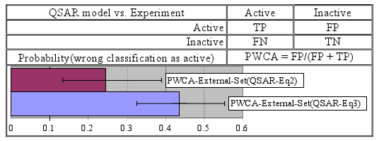
- ▪ The smallest value of the probability of wrong classification as an active compound was obtained in the training set while the highest value was obtained in the external set (these two probabilities proved significantly different).
- ▪ The smallest value of the probability of wrong classification as an inactive compound was obtained in test set. No statistically significant difference in terms of the probability of wrong classification was identified when all three sets of compounds were analyzed.
- ▪ The odds of correct classification in the group of active compounds divided by the odds of incorrect classification in the group of inactive compounds proved to be almost identical in the training and external sets. Even if the value of the odds ratio obtained in test set is higher than the values obtained in training or external sets, the ability of our classification model in terms of OR proved not to be significantly different in this set (the confidence intervals overlap one another).
- ▪ The interdependence between the observed and estimated/predicted class (active/inactive) was proved statistically for both models (Equation 3–Table 1 and Equation 2–Table 2) but the correlation coefficients in the 2 × 2 contingency table proved to be higher for the model presented in Equation 2.
- ▪ The higher accuracy for all three sets sustains the use of model presented in Equation 2 in the classification of active and inactive BBB compounds. The accuracy seems not to be statistically significantly different when the model from Equation 3 is compared to the model from Equation 2 since the associated 95% confidence intervals overlap one another.
- ▪ The under-classification as well as over-classification seems to have the smallest values for the model from Equation 2 compared to the model from Equation 3, but since the associated 95% confidence intervals overlap one another these differences do not seem to be statistically significant.
- ▪ The percentage of compounds correctly assigned as active out of all of those assigned as active proved to be higher for the model presented in Equation 2 compared to the model presented in Equation 3. Since the 95% confidence intervals overlap one another, these percentages are not statistically significantly different. The same observation is also true for the percentage of compounds correctly assigned as inactive out of all of those assigned as inactive.
- ▪ The previously reported model seems to have the smallest probabilities of wrong classification as active/inactive compounds. However, based on the overlap of associated 95% confidence interval it could be that these differences are not statistically significant.
4. Experimental Section
4.1. Classification Model—Predictivity Approach
4.2. Classification Model as Comparison Tool
4.3. Datasets and BBB Permeation Property
4.4. Molecular Descriptors Calculation
5. Conclusions
Acknowledgements
References
- Rubin, LL; Staddon, JM. The cell biology of the blood-brain barrier. Annu. Rev. Neurosci 1999, 22, 11–28. [Google Scholar]
- Abraham, MH; Ibrahim, A; Zhao, Y; Acree, WE. A data base for partition of volatile organic compounds and drugs from blood/plasma/serum to brain, and an LFER analysis of the data. J. Pharm. Sci 2006, 95, 2091–2100. [Google Scholar]
- Klon, AE. Computational models for central nervous system penetration. Curr. Comput.-Aided Drug Des 2009, 5, 71–89. [Google Scholar]
- Bechtold, E; Reisz, JA; Klomsiri, C; Tsang, AW; Wright, MW; Poole, LB; Furdui, CM; King, SB. Water-soluble triarylphosphines as biomarkers for protein s-nitrosation. ACS Chem. Biol 2010, 5, 405–414. [Google Scholar]
- Clark, DE. In silico prediction of blood-brain barrier permeation. Drug Discov. Today 2003, 8, 927–933. [Google Scholar]
- Young, RC; Mitchell, RC; Brown, TH; Ganellin, CR; Griffiths, R; Jones, M; Rana, KK; Saunders, D; Smith, IR; Sore, NE; et al. Development of a new physicochemical model for brain penetration and its application to the design of centrally acting H2 receptor histamine antagonists. J. Med. Chem 1988, 31, 656–671. [Google Scholar]
- Crivori, P; Cruciani, G; Carrupt, PA; Testa, B. Predicting blood-brain barrier permeation from three-dimensional molecular structure. J. Med. Chem 2000, 43, 2204–2216. [Google Scholar]
- Narayanan, R; Gunturi, SB. In silico ADME modelling: prediction models for blood-brain barrier permeation using a systematic variable selection method. Bioorg. Med. Chem 2005, 13, 3017–3028. [Google Scholar]
- Subramanian, G; Kitchen, DB. Computational models to predict blood-brain barrier permeation and CNS activity. J. Comput.-Aided Mol. Des 2003, 17, 643–664. [Google Scholar]
- Goodwin, JT; Clark, DE. In silico predictions of blood-brain barrier penetration: Considerations to “keep in mind”. J. Pharmacol. Exp. Ther 2005, 315, 477–483. [Google Scholar]
- Semple, G; Andersson, BM; Chhajlani, V; Georgsson, J; Johansson, MJ; Rosenquist, A; Swanson, L. Synthesis and biological activity of kappa opioid receptor agonists. Part 2: preparation of 3-aryl-2-pyridone analogues generated by solutionand solid-phase parallel synthesis methods. Bioorg. Med. Chem. Lett 2003, 13, 1141–1145. [Google Scholar]
- Perioli, L; Ambrogi, V; Bernardini, C; Grandolini, G; Ricci, M; Giovagnoli, S; Rossi, C. Potential prodrugs of non-steroidal anti-inflammatory agents for targeted drug delivery to the CNS. Eur. J. Med. Chem 2004, 39, 715–727. [Google Scholar]
- Hodgetts, KJ; Yoon, T; Huang, J; Gulianello, M; Kieltyka, A; Primus, R; Brodbeck, R; De Lombaert, S; Doller, D. 2-Aryl-3,6-dialkyl-5-dialkylaminopyrimidin-4-ones as novel crf-1 receptor antagonists. Bioorg. Med. Chem. Lett 2003, 13, 2497–2500. [Google Scholar]
- Zhang, H; Hu, S; Zhang, Y. Prediction of distribution of neutral, acidic and basic structurally diverse compounds between blood and brain by the nonlinear methodology. Med. Chem 2008, 4, 170–189. [Google Scholar]
- Klon, AE. Computational Models for Central Nervous System Penetration. Curr. Comput.-Aided Drug Des 2009, 5, 71–89. [Google Scholar]
- Fan, Y; Unwalla, R; Denny, RA; Di, L; Kerns, EH; Diller, DJ; Humblet, C. Isights for predicting blood-brain barrier penetration of CNS targeted molecules using QSPR approaches. J. Chem. Inf. Model 2010, 50, 1123–1133. [Google Scholar]
- Lanevskij, K; Dapkunas, J; Juska, L; Japertas, P; Didziapetris, R. QSAR analysis of blood-brain distribution: The influence of plasma and brain tissue binding. J. Pharm. Sci 2011, 100, 2147–2160. [Google Scholar]
- Smye, SW; Clayton, RH. Mathematical modelling for the new millenium: Medicine by numbers. Med. Eng. Phys 2002, 24, 565–574. [Google Scholar]
- Sarbu, C. A comparative-study of regression concerning weighted least-squares methods. Anal. Lett 1995, 28, 2077–2094. [Google Scholar]
- Okuno, Y. In silico drug discovery based on the integration of bioinformatics and chemoinformatics. Yakugaku Zasshi-J. Pharm. Soc. Jpn 2008, 128, 1645–1651. [Google Scholar]
- Gozalbes, R; Carbajo, RJ; Pineda-Lucena, A. Contributions of computational chemistry and biophysical techniques to fragment-based drug discovery. Curr. Med. Chem 2010, 17, 1769–1794. [Google Scholar]
- Loving, K; Alberts, I; Sherman, W. Computational approaches for fragment-based and de novo design. Curr. Top. Med. Chem 2010, 10, 14–32. [Google Scholar]
- Sun, H; Scott, DO. Structure-based drug metabolism predictions for drug design. Chem. Biol. Drug Des 2010, 75, 3–17. [Google Scholar]
- Taherpour, A. Theoretical and quantitative structural relationship studies of electrochemical properties of the nanostructures of cis-unsaturated thiocrown ethers and their supramolecular complexes [X-UT-Y][M@C82] (M = Ce, Gd). Phosphorus, Sulfur Silicon Relat. Elem 2010, 185, 422–432. [Google Scholar]
- Taherpour, AA; Taherpour, A; Taherpour, Z; Taherpour, O. Relationship study of octanol-water partitioning coefficients and total biodegradation of linear simple conjugated polyene and carotene compounds by use of the Randic index and maximum UV wavelength. Phys. Chem. Liq 2009, 47, 349–359. [Google Scholar]
- Hawkins, DM. The problem of overfitting. J. Chem. Inf. Comput. Sci 2004, 44, 1–12. [Google Scholar]
- Durbin, J; Watson, GS. Testing for serial correlation in least squares regression, I. Biometrika 1950, 37, 409–428. [Google Scholar]
- Durbin, J; Watson, GS. Testing for serial correlation in least squares regression, II. Biometrika 1951, 38, 159–179. [Google Scholar]
- Picard, R; Cook, D. Cross-validation of regression models. J. Am. Stat. Assoc 1984, 79, 575–583. [Google Scholar]
- Kortagere, S; Chekmarev, D; Welsh, WJ; Ekins, S. New predictive models for blood-brain barrier permeability of drug-like molecules. Pharm. Res 2008, 25, 1836–1845. [Google Scholar]
- Cooper, JA; Saracci, R; Cole, P. Describing the validity of carcinogen screening tests. Br. J. Cancer 1979, 39, 87–89. [Google Scholar]
- Bolboacă, S; Jäntschi, L; Achimaş Cadariu, A. Creating diagnostic critical appraised topics. catrom original software for romanian physicians. Appl. Med. Inf 2004, 14, 27–34. [Google Scholar]
- Drugan, T; Bolboacă, S; Jäntschi, L; Achimaş Cadariu, A. Binomial distribution sample confidence intervals estimation 1. sampling and medical key parameters calculation. Leonardo Electron. J. Pract. Technol 2003, 3, 47–74. [Google Scholar]
- Bolboacă, S; Jäntschi, L. Optimized confidence intervals for binomial distributed samples. Int. J. Pure Appl. Math 2008, 47, 1–8. [Google Scholar]
- Jäntschi, L; Bolboacă, SD. Exact probabilities and confidence limits for binomial samples: Applied to the difference between two proportions. The Scientific World JOURNAL 2010, 10, 865–878. [Google Scholar]
- Steiger, JH. Tests for comparing elements of a correlation matrix. Psychol. Bull 1980, 87, 245–251. [Google Scholar]
- Iyer, M; Mishru, R; Han, Y; Hopfinger, AJ. Predicting blood-brain barrier partitioning of organic molecules using membrane-interaction QSAR analysis. Pharm. Res 2002, 19, 1611–1621. [Google Scholar]
- Liu, X; Tu, M; Kelly, RS; Chen, C; Smith, BJ. Development of a computational approach to predict blood-brain barrier permeability. Drug Metab. Dispos 2004, 32, 132–139. [Google Scholar]
- Rose, K; Hall, LH; Hall, LM; Kier, LB. Modeling blood-brain barrier partitioning using topological structure descriptors. Available online: http://www.symyx.com/products/pdfs/qsar_whitepaper2.pdf accessed on 11 June 2010.
- Bolboacă, SD; Jäntschi, L. Computer assisted geometry optimization for in silico modeling. Comput Methods Progr Biomed 2010. submitted for publication. [Google Scholar]
- Bolboacă, SD; Jäntschi, L. Comparison of quantitative structure-activity relationship model performances on carboquinone derivatives. The Scientific World JOURNAL 2009, 9, 1148–1166. [Google Scholar]
- Bolboacă, SD; Jäntschi, L. Modelling the property of compounds from structure: statistical methods for models validation. Environ. Chem. Lett 2008, 6, 175–181. [Google Scholar]

| Parameter (Abbreviation) | Equation | Training Set (n = 81) [95%CI] | Test Set (n = 41) [95%CI] | External Set (n = 315) [95%CI] |
|---|---|---|---|---|
| χ2 statistic (p-value) | 10.29 (0.0013) | 7.75 (0.0054) | 28.24 (p < 0.0001) | |
| Φ | 0.3564 | 0.4347 | 0.2994 | |
| Accuracy (AC) | 5 | 69.14 [58.53–78.37] | 73.17 [58.32–84.77] | 72.70 [67.58–77.39] |
| Error Rate (ER) | 6 | 30.86 | 26.83 | 27.30 |
| Prior proportional probability of | 7 | |||
| -an active class | 0.482 [0.371–0.592] | 0.463 [0.318–0.614] | 0.302 [0.253–0.354] | |
| -an inactive class | 0.519 [0.408–0.630] | 0.537 [0.367–0.682] | 0.698 [0.644–0.749] | |
| Sensitivity (Se) | 8 | 64.10 [48.47–77.70] | 84.21 [63.16–95.05] | 42.11 [32.54–52.15] |
| False-negative rate (under-classification, FNR) | 9 | |||
| 35.90 [22.30–45.51] | 15.79 [4.95–36.84] | 57.89 [47.85–67.46] | ||
| Specificity (Sp) | 10 | 73.81 [59.20–85.15] | 63.64 [42.87–81.04] | 85.91 [80.80–89.98] |
| False-positive rate (over-classification, FPR) | 11 | |||
| 26.19 [14.86–40.80] | 36.36 [0.1896–0.5712] | 14.09 [10.02–19.20] | ||
| Positive predictivity (PP) | 12 | 69.44 [53.32–82.51] | 66.67 [46.76–82.76] | 56.34 [44.74–67.43] |
| Negative predictivity (NP) | 13 | 68.89 [54.49–80.89] | 82.35 [59.63–97.48] | 77.46 [72.59–81.80] |
| Post-test probability of classification | 14 | |||
| -as active (PCA) | 0.444 [0.340–0.553] | 0.585 [0.433–0.726] | 0.225 [0.177–0.281] | |
| -as inactive (PCIC) | 0.556 [0.447–0.660] | 0.415 [0.274–0.567] | 0.775 [0.7259–0.818] | |
| Probability of a wrong classification | 15 | |||
| -as active compound (PWCA) | 0.306 [0.175–0.467] | 0.333 [0.172–0.532] | 0.437 [0.326–0.553] | |
| -as inactive compound (PWCI) | 0.311 [0.191–0.455] | 0.177 [0.055–0.404] | 0.225 [0.177–0.281] | |
| Odds Ratio (OR) | 16 | 5.03 [1.96–13.12] | 9.33 [2.18–40.07] | 4.43 [2.53–7.76] |
| Parameter (Abbreviation) | Equation | Training (n = 88) | Test (n = 28) | External (n = 92) |
|---|---|---|---|---|
| χ2 statistic (p-value) | 30.91 (p < 0.0001) | 9.82 (0.0017) | 28.76 (p < 0.0001) | |
| Φ | 0.5927 | 0.5922 | 0.5591 | |
| Accuracy (AC) | 5 | 80.68 [71.45–87.80] | 92.86 [78.12–98.17] | 79.35 [70.19–86.58] |
| Error Rate (ER) | 6 | 19.32 | 7.14 | 20.65 |
| Prior proportional probability of | 7 | |||
| -an active class | 0.511 [0.408–0.614] | 0.179 [0.074–0.350] | 0.435 [0.337–0.537] | |
| -an inactive class | 0.489 [0.375–0.602] | 0.821 [0.644–0.927] | 0.565 [0.457–0.674] | |
| Sensitivity (Se) | 8 | 77.78 [64.06–87.87] | 60.00 [20.97–90.51] | 77.50 [62.85–88.14] |
| False-negative rate (under-classification, FNR) | 9 | |||
| 22.22 [12.13–35.94] | 40.00 [9.49–79.03] | 22.50 [11.86–37.15] | ||
| Specificity (Sp) | 10 | 83.72 [70.48–92.25] | 100.00 [87.79–100.00] | 80.77 [68.45–89.55] |
| False-positive rate (over-classification, FPR) | 11 | |||
| 16.28 [7.78–29.52] | 0.00 [0.00–12.21] | 19.23 [10.45–31.55] | ||
| Positive predictivity (PP) | 12 | 83.33 [70.48–92.25] | 100.00 [36.84–100.00] | 75.61 [60.69–86.63] |
| Negative predictivity (NP) | 13 | 78.26 [64.76–88.14] | 92.00 [75.85–97.97] | 82.35 [70.12–90.77] |
| Post-test probability of classification | 14 | 0.477 [0.375–0.581] | ||
| -as active (PCA) | 0.523 [0.419–0.625] | 0.107 [0.034–0.265] | 0.446 [0.347–0.548] | |
| -as inactive (PCIC) | 0.477 [0.375–0.581] | 0.893 [0.735–0.966] | 0.554 [0.452–0.653] | |
| Probability of a wrong classification | 15 | |||
| -as active compound (PWCA) | 0.167 [0.079–0.302] | 0.000 [0.000–0.122] | 0.244 [0.134–0.390] | |
| -as inactive compound (PWCI) | 0.217 [0.119–0.352] | 0.080 [0.020–0.242] | 0.177 [0.092–0.299] | |
| Odds Ratio (OR) | 16 | 18.00 [6.25–52.39] | n.a. | 14.47 [5.32–39.99] |
| Parameter (Abbreviation) | Formula | Definition | Equation |
|---|---|---|---|
| Concordance/Accuracy/Non-error Rate (CC/AC) | 100 × (TP + TN)/n | Total fraction of compounds correctly classified | 6 |
| Error Rate (ER) | 100 × (FP + FN)/n = 1 − CC | Total fraction of compounds misclassified | 7 |
| Prior proportional probability of a class (PPP) | ni/n | Fraction of compounds belonging to class i | 8 |
| Sensitivity (Se) | 100 × TP/(TP + FN) | Percentage of BBB+ compounds correctly assigned to the active class | 9 |
| False-negative rate (under-classification, FNR) | 100 × FN/(TP + FN) = 1 − Se | percentage of BBB+ compounds falsely assigned to the non-active class | 10 |
| Specificity (Sp) | 100 × TN/(TN + FP) | Percentage of BBB– compounds correctly assigned to the negative class | 11 |
| False-positive rate (over-classification, FPR) | 100 × FP/(FP + TN) = 1 − Sp | Percentage of BBB– compounds falsely assigned to be active | 12 |
| Positive predictivity (PP) | 100 × TP/(TP + FP) | Percentage of compounds correctly assigned as active out of all active assigned compounds | 13 |
| Negative predictivity (NP) | 100 × TN/(TN + FN) | Percentage of non-active out of non-active assigned compounds | 14 |
| Probability of classification | 15 | ||
| as active (PCA) | (TP + FP)/n | - Probability to classify a compound as active (true positive & false positive) | |
| as inactive (PCIC) | (FN + TN)/n | - Probability to classify a compound as inactive (true negative & false negative) | |
| Probability of a wrong classification | 16 | ||
| as active compound (PWCA) | FP/(FP + TP) | Probability of a false positive classification | |
| as inactive compound (PWCI) | FN/(FN + TN) | Probability of a false negative classification | |
| Odds Ratio (OR) | (TP × TN)/(FP × FN) | The odds of correct classification in the group of active compounds divided to the odds of a incorrect classification in the group of inactive compounds | 17 |
| No. | Name | ID | logBB | Set | Ref. |
|---|---|---|---|---|---|
| 1 | Cimetidine | CID: 2756 | −1.42 | 2 | [37] |
| 2 | Icotidine | CID: 72108 | −2.00 | 1 | [37] |
| 3 | Lupitidine | CID: 51671 | −1.06 | 2 | [8] |
| 4 | Clonidine | CID: 2803 | 0.11 | 1 | [37] |
| 5 | Mepyramine | CID: 4992 | 0.49 | 1 | [37] |
| 6 | Imipramine | CID: 3696 | 0.83 | 1 | [37] |
| 7 | Ranitidine | CID: 5039 | −1.23 | 2 | [37] |
| 8 | Tiotidine | CID: 50287 | −0.82 | 1 | [37] |
| 9 | Zolantidine | CID: 91769 | 0.14 | 2 | [37] |
| 10 | Butanone | CID: 6569 | −0.08 | 2 | [8] |
| 11 | Benzene | CID: 241 | 0.37 | 1 | [8] |
| 12 | 3-Methylpentane | CID: 7282 | 1.01 | 1 | [8] |
| 13 | 3-Methylhexane | CID: 11507 | 0.90 | 1 | [8] |
| 14 | 2-Propanol | CID: 3776 | −0.15 | 1 | [8] |
| 15 | 2-Methylpropanol | CID: 6560 | −0.17 | 1 | [8] |
| 16 | 2-Methylpentane | CID: 7892 | 0.97 | 2 | [8] |
| 17 | 2,2-Dimethylbutane | CID: 580244 | 1.04 | 2 | [8] |
| 18 | 1,1,1-Trichloroethane | CID: 6278 | 0.40 | 1 | [37] |
| 19 | Diethyl ether | CID: 3283 | 0.00 | 2 | [8] |
| 20 | Enflurane | CID: 3226 | 0.24 | 1 | [8] |
| 21 | Ethanol | CID: 702 | −0.16 | 2 | [8] |
| 22 | Fluroxene | CID: 9844 | 0.13 | 1 | [8] |
| 23 | Halothane | CID: 3562 | 0.35 | 1 | [8] |
| 24 | Heptane | CID: 8900 | 0.81 | 1 | [8] |
| 25 | Hexane | CID: 8058 | 0.80 | 2 | [8] |
| 26 | Isoflurane | CID: 3763 | 0.42 | 2 | [8] |
| 27 | Methylcyclopentane | CID: 7296 | 0.93 | 2 | [8] |
| 28 | Nitrogen | CID: 947 | 0.03 | 1 | [8] |
| 29 | Pentane | CID: 8003 | 0.76 | 2 | [8] |
| 30 | n-Propanol | CID: 1031 | −0.16 | 2 | [8] |
| 31 | Propanone | CID: 180 | −0.15 | 2 | [8] |
| 32 | Teflurane | CID: 31300 | 0.27 | 1 | [8] |
| 33 | Toluene | CID: 1140 | 0.37 | 1 | [8] |
| 34 | Acetylsalicylic acid | CID: 2244 | −0.50 | 1 | [8] |
| 35 | Pentobarbital | CID: 4737 | 0.12 | 1 | [8] |
| 36 | Physostigmine | CID: 5983 | 0.08 | 2 | [8] |
| 37 | Salicylic acid | CID: 338 | −1.10 | 1 | [8] |
| 38 | Trifluoro Perazine | CID: 5566 | 1.44 | 1 | [8] |
| 39 | Valproic acid | CID: 3121 | −0.22 | 1 | [8] |
| 40 | Verapamil | CID: 2520 | −0.70 | 1 | [8] |
| 41 | Zidovudine | CID: 5726 | −0.72 | 1 | [8] |
| 42 | Hydroxyzine | CID: 3658 | 0.39 | 2 | [8] |
| 43 | Thioridazine | CID: 5452 | 0.24 | 1 | [8] |
| 44 | Alprazolam | CID: 2118 | 0.04 | 2 | [8] |
| 45 | Phenserine | CID: 192706 | 1.00 | 1 | [8] |
| 46 | Midazolam | CID: 4192 | 0.36 | 2 | [8] |
| 47 | Codeine | CID: 5284371 | 0.55 | 2 | [8] |
| 48 | Chlorpromazine | CID: 2726 | 1.06 | 2 | [8] |
| 49 | Promazine | CID: 4926 | 1.23 | 1 | [8] |
| 50 | Nevirapine | CID: 4463 | 0.00 | 1 | [8] |
| 51 | Thioperamide | CID: 3035905 | −0.16 | 1 | [8] |
| 52 | Didanosine | CID: 3043 | −1.30 | 2 | [8] |
| 53 | Ibuprofen | CID: 3672 | −0.18 | 1 | [8] |
| 54 | Antipyrine | CID: 2206 | −2.00 | 2 | [38] |
| 55 | Theophyline | CID: 2153 | −0.29 | 1 | [8] |
| 56 | p-Acetamido phenol | CID: 1983 | −0.31 | 1 | [8] |
| 57 | Nitrous Oxide | CID: 948 | 0.03 | 1 | [8] |
| 58 | Carbon bisulphide | CID: 6348 | 0.60 | 1 | [8] |
| 59 | Indomethacin | CID: 3715 | −1.26 | 1 | [8] |
| 60 | Indinavir | CID: 5362440 | −0.75 | 1 | [8] |
| 61 | Oxazepam | CID: 4616 | 0.61 | 1 | [8] |
| 62 | Carbamazepine | CID: 2554 | −0.14 | 2 | [39] |
| 63 | Carbamazepine epoxide | CID: 2555 | −0.35 | 1 | [39] |
| 64 | Amitriptyline | CID: 2160 | 0.88 | 1 | [8] |
| 65 | Desipramine | CID: 2995 | 1.00 | 1 | [8] |
| 66 | Mianserin | CID: 4184 | 0.99 | 2 | [8] |
| 67 | ORG 4428 | CID: 166560 | 0.82 | 2 | [8] |
| 68 | Mirtazapine | CID: 4205 | 0.53 | 1 | [8] |
| 69 | Tibolone | CID: 21844 | 0.40 | 1 | [8] |
| 70 | Domperidone | CID: 3151 | −0.78 | 2 | [8] |
| 71 | Risperidone | CID: 5073 | −0.67 | 2 | [8] |
| 72 | 9-OH-Risperidone | CID: 475100 | −0.02 | 1 | [8] |
| 73 | Temelastine | CID: 55482 | −1.88 | 2 | [8] |
| 74 | BBCPD13 | CSID: 14922095 | −0.66 | 1 | [37] |
| 75 | BBCPD15 | CSID: 2992532 | −0.18 | 1 | [37] |
| 76 | BBCPD57 | CSID: 10439135 | −1.15 | 2 | [37] |
| 77 | BBCPD58 | CSID: 10442225 | −1.54 | 1 | [37] |
| 78 | BBCPD17 | CSID: 10442293 | −1.12 | 1 | [37] |
| 79 | BBCPD20 | CID: 9971484 | −0.46 | 1 | [37] |
| 80 | BBCPD21 | CID: 10498206 | −0.24 | 2 | [37] |
| 81 | SB222200 | CSID: 3167851 | 0.30 | 1 | [8] |
| 82 | Y-G14 | CSID: 2276 | −0.30 | 1 | [8] |
| 83 | Y-G15 | CSID: 72747 | −0.06 | 1 | [37] |
| 84 | Caffeine | CID: 2519 | −2.00 | 1 | [38] |
| 85 | Chlorambucil | CID: 2708 | −1.60 | 1 | [38] |
| 86 | Glycine | CID: 750 | −3.50 | 2 | [38] |
| 87 | Morphine | CID: 5288826 | −2.70 | 2 | [38] |
| 88 | Phenylalanine | CID: 994 | −1.30 | 2 | [38] |
| 89 | Phenytoin | CID: 1775 | −2.20 | 1 | [38] |
| 90 | Propranolol | CID: 4946 | −1.20 | 1 | [38] |
| 91 | Taurocholic Acid | CID: 444349 | −4.10 | 1 | [38] |
| 92 | Trichloroethylene | CID: 6575 | 0.34 | 1 | [37] |
| 93 | Carmustine | CID: 450682 | −0.52 | 1 | [39] |
| 94 | ORG34167 | CSID: 8036856 | 0.00 | 1 | [8] |
| 95 | BBCPD22 | CSDI: 8620184 | −0.02 | 1 | [37] |
| 96 | BBCPD23 | BBCPD23 | 0.69 | 2 | [37] |
| 97 | BBCPD24 | BBCPD24 | 0.44 | 1 | [37] |
| 98 | BBCPD26 | BBCPD26 | 0.22 | 2 | [37] |
| 99 | 1,1,1-Trifluoro-2-chloro ethane | CSID: 6168 | 0.08 | 1 | [37] |
| 100 | T7 | T7 | 0.85 | 1 | [37] |
| 101 | BBCPD60 | CSDI: 23218171 | −0.73 | 1 | [37] |
| 102 | BBCPD18 | BBCPD18 | −0.27 | 1 | [37] |
| 103 | BBCPD19 | BBCPD19 | −0.28 | 2 | [37] |
| 104 | BBCPD16 | BBCPD16 | −1.57 | 1 | [37] |
| 105 | BBCPD14 | BBCPD14 | −0.12 | 2 | [37] |
| 106 | Y-G16 | Y-G16 | −0.42 | 1 | [8] |
| 107 | Y-G19 | Y-G19 | −1.30 | 2 | [8] |
| 108 | Y-G20 | CSID: 5854406 | −1.40 | 1 | [37] |
| 109 | SKF89124 | CSID: 117961. | −0.43 | 1 | [8] |
| 110 | SKF101468 | CSID: 4916 | 0.25 | 1 | [37] |
| 111 | CBZ-EPO | CBZ-EPO | −0.34 | 1 | [37] |
| 112 | L-663581 | CSID: 114837 | −0.30 | 1 | [8] |
| 113 | M1L-663,581 | CSID: 8560187 | −1.34 | 1 | [37] |
| 114 | M2L-663581 | CSID: 8267285 | −1.82 | 1 | [8] |
| 115 | ORG5222 | ORG5223 | 1.03 | 2 | [8] |
| 116 | ORG12962 | CSID: 7972174 | 1.64 | 1 | [8] |
| 117 | ORG13011 | ORG13011 | 0.16 | 1 | [8] |
| 118 | ORG32104 | ORG32104 | 0.52 | 1 | [8] |
| 119 | ORG30526 | ORG30526 | 0.39 | 1 | [8] |
| 120 | ICI17148 | ICI17149 | −0.04 | 2 | [37] |
| 121 | SK&F93319 | SK&F93320 | −1.30 | 1 | [37] |
| 122 | CBZ | CBZ | 0.00 | 1 | [37] |
| Parameter | Training set (n = 81) | Test set (n = 41) |
|---|---|---|
| m [95%CI] | −0.2003 [−0.4060; −0.0055] | −0.2529 [−0.5916; 0.0858] |
| StDev | 0.9306 | 1.0731 |
| Min | −4.10 | −3.50 |
| Max | 1.64 | 1.06 |
| KS statistic (p) | 0.1151 (0.2163) | 0.1729 (0.1531) |
| AD statistic * | 1.1582 * | 0.9939 * |
| CS statistic (p) | 8.1850 (0.2249) | 0.3650 (0.9852) |
© 2011 by the authors; licensee MDPI, Basel, Switzerland. This article is an open-access article distributed under the terms and conditions of the Creative Commons Attribution license (http://creativecommons.org/licenses/by/3.0/).
Share and Cite
Bolboacă, S.D.; Jäntschi, L. Predictivity Approach for Quantitative Structure-Property Models. Application for Blood-Brain Barrier Permeation of Diverse Drug-Like Compounds. Int. J. Mol. Sci. 2011, 12, 4348-4364. https://doi.org/10.3390/ijms12074348
Bolboacă SD, Jäntschi L. Predictivity Approach for Quantitative Structure-Property Models. Application for Blood-Brain Barrier Permeation of Diverse Drug-Like Compounds. International Journal of Molecular Sciences. 2011; 12(7):4348-4364. https://doi.org/10.3390/ijms12074348
Chicago/Turabian StyleBolboacă, Sorana D., and Lorentz Jäntschi. 2011. "Predictivity Approach for Quantitative Structure-Property Models. Application for Blood-Brain Barrier Permeation of Diverse Drug-Like Compounds" International Journal of Molecular Sciences 12, no. 7: 4348-4364. https://doi.org/10.3390/ijms12074348