Introducing Catastrophe-QSAR. Application on Modeling Molecular Mechanisms of Pyridinone Derivative-Type HIV Non-Nucleoside Reverse Transcriptase Inhibitors

Abstract
:
1. Introduction
2. Background Theories
2.1. QSAR Phenomenology
- Y stands for the computed activity, not the observed activity, from the statistical characteristics of the present approach; thus the validation of Equation (1) should be done for another (preferably external or testing) set of compounds with which the predictive power of Equation (1) is tested.
- Because the right side of Equation (1) unfolds as a linear summation of the structural characteristics, it corresponds in fact with the quantum superposition principle, which provides a global Eigen-solution for a quantum system from its particular realization in orthogonal or projective sub-space; from where the need arises for structural indices X1, ..., XM to be either linearly independent or orthogonal in algebraic space built from their associate vectors presented in Table 1.
- QSAR 1: a defined endpoint
- QSAR-2: an unambiguous algorithm
- QSAR-3: a defined domain of applicability
- QSAR-4: appropriate measures of goodness-of–fit, robustness and predictivity
- QSAR-5: a mechanistic interpretation, if possible
- QSAR-1. why does one do modeling ?
- QSAR-2. how does one do modeling ?
- QSAR-3. with what tools do I model ?
- QSAR-4. how reliable is what I modeled ?
- QSAR-5. what knowledge did the model provide ?
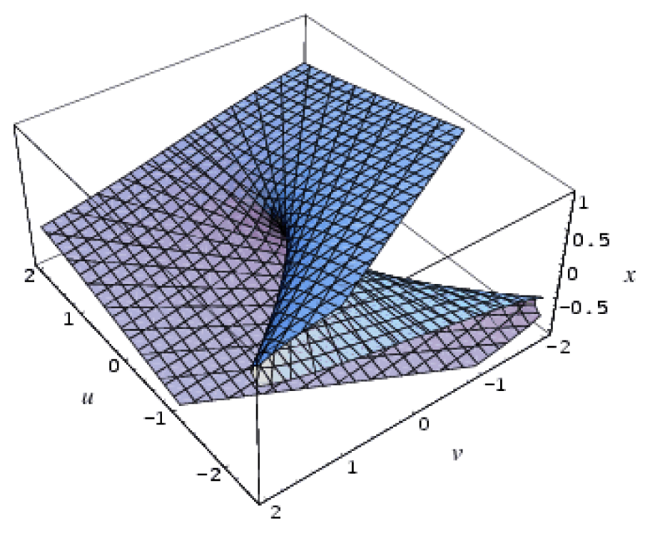
2.2. Thom’s Catastrophe Theory
3. Catastrophe-QSAR Method
- Determine the norms for each model
- Calculate the algebraic correlation factor for each model [31]
- Calculate the so-called “statistical relative power” index for each model with each set of descriptorswhere the components are defined as follows:
- relative index of correlation:
- relative index for Student’s t-test
- relative index for Fisher’s test
- Determine the generalized Euclidian distances between corresponding type-I and type-II models employing different descriptorsand establish formal matrices for the models’ differences for single descriptors, respectivelywhereand for pair descriptors
- Identify all minimum paths across all differences ΔΠI (X1∨X2), Δ2ΠI(X1,X2) and ΔΠII(X1∧X2) for a given set of descriptors (X1, X2)The combination of descriptors that fulfills this system provides the molecular mechanism of the interaction. The correlation models involved are ordered according to their relative statistical power within the same molecular mechanism, thereby providing the best models. Because pair-descriptors are primarily involved in the present analysis, one can consider the first two such “waves” and their best correlation models up to the second order minimum paths, as in Equation (16).
- For selected correlation models, in either structure-driven or molecular mechanistic “waves,” one employs them to compute the associated predicted activities for test molecules and to provide the statistics regarding the observed activity. If the obtained relative statistical power is close to those characteristic for the trial set of molecules, then these models may be validated for the specific eco-, bio-, or pharmacological problem. Moreover, further insight will be provided by the analysis of the catastrophe shape of the models involved and discussed accordingly.
4. Application to Non-Nucleoside Reverse Transcriptase Pyridinone Inhibitors
4.1. Input Data
4.2. Results and Discussion
- - First, it is clear that consideration of the catastrophe (polynomial) correlations is an improvement over the old multi-linear QSAR statistics (see also Appendix-A2).
- - The hydrophobicity indicator gives generally low correlations with any polynomial (linear, multilinear or catastrophe) approach, being a quite irrelevant linear QSAR descriptor (Table 5) but improving up to twice its influence within the swallow tail and butterfly phenomenologies once its fifth and sixth power involvement are considered. Nevertheless, this provides a sign of the value of catastrophe-QSAR for achieving a deeper understanding of the molecular mechanics of specific interactions when the normal multi-linear QSAR does not assign transport descriptors with much predictive power.
- - The relative statistical power, as defined by Equation (8), does not always parallel the Pearson coefficient or the relative correlation factors, as is evident from Tables 5 and 6. However, because it includes more statistical information, we consider a model as relevant when it has greater individual output of this newly introduced statistical index. In particular, neither the linear nor the multilinear QSAR framework provides a good fit between the statistical correlation and the relative statistical power using the structural parameter combinations considered. Instead, parabolic catastrophe correlations, the cusp and butterfly models, are revealed to be quite relevant, in particular regarding the formation energy (H) for which they show the highest Pearson correlation and relative statistical power values in comparison with the other descriptors plugged into these models. Unfortunately, for the two-variable descriptor models of Table 6, no consistency was found between the highest Pearson value and the relative statistical power apart from a few degenerate cases of descriptors for the parabolic models where the highest relative statistical power value corresponds with the highest Pearson correlation. Note that for the degenerate cases of Table 6, when two mixed descriptors can be combined in two distinct ways, the working model is considered to have maximum relative statistical power.
- - Table 7: At the individual descriptor level, the cusp and butterfly models are very close to each other for Log P and the forming energy H, which is even more relevant for the hydrophobicity, because for the forming energy it transpires from Table 5 that the butterfly model practically reduces to the cusp model because the sixth contribution virtually vanishes. However, for the structural influence on polarizability (POL) the butterfly and swallow tail are the closest models. When one considers the hierarchy of the individual descriptors according to their QSAR-I models in Table 5 in terms of the reduction in relative statistical power
- - Table 8: When the second order distance difference is considered between the individual inter-modeling paths of Table 7, it can nevertheless be considered through the further variations of paths of Table 7. Also, the QSAR-I and the fold (F) catastrophe model intervene in changing the influence on specific interactions from POL to H. Therefore, by counting the minimum hierarchy of these paths, the distance ordering is obtained as follows:
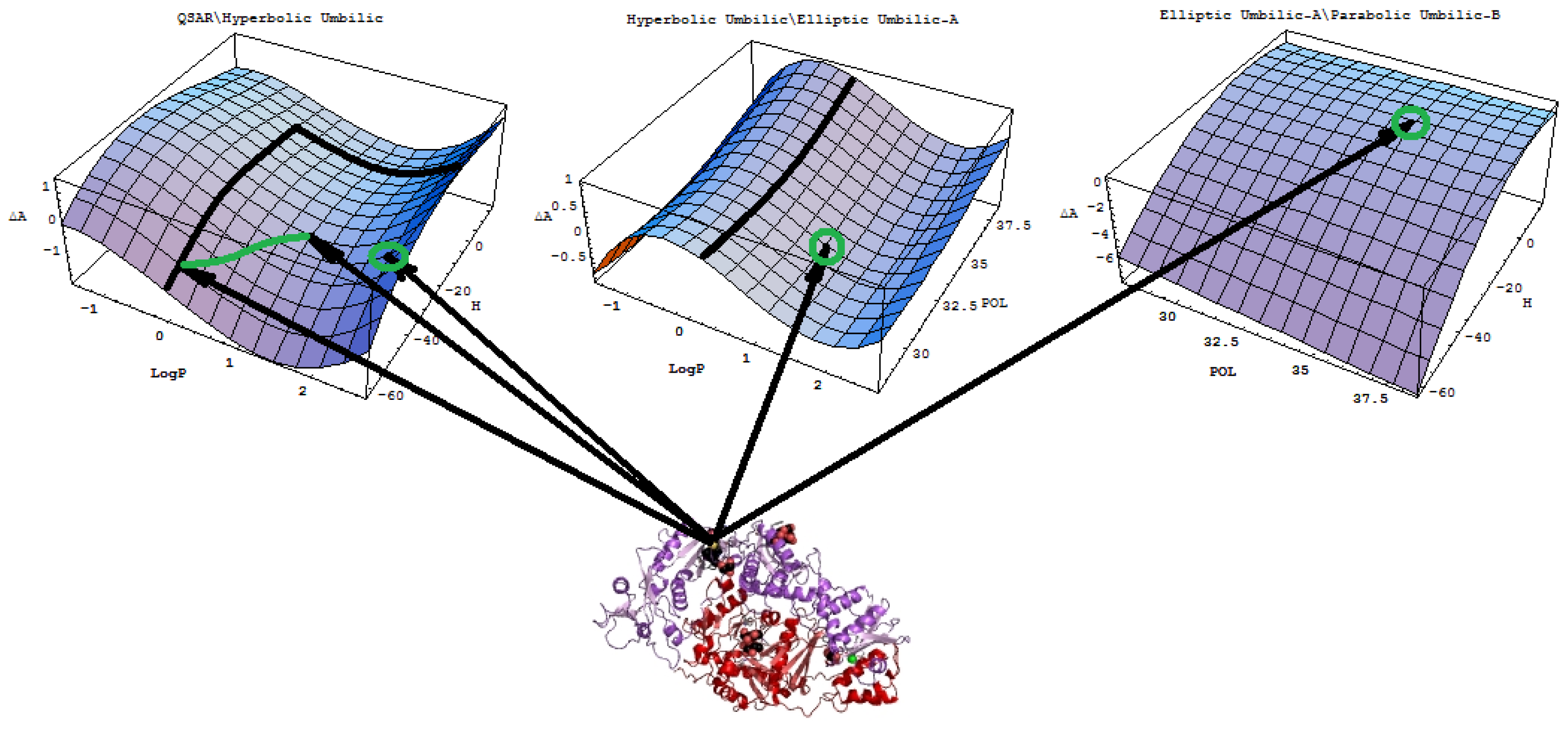
- The HIV-1 inhibitory activity is triggered by a hydrophobic interaction followed by energetic stabilization of the ligand/substrate (pyrididone derivative/viral protein) interaction here modeled by the heat of molecular formation and eventually completed by the ionic field influence herein represented by the polarizability descriptor.
- Although the QSAR multi-linear model should not be excluded from the molecular modeling of complex bio-chemical interactions, it should be complemented with other polynomial correlational catastrophe-type models that produce significant results comparable to those of other 3D-modeling procedures such as docking-based comparative molecular field analysis (CoMFA) and comparative molecular similarity indices analysis (CoMSIA) [24].
- Log P: For positive values, the compound behaves hydrophobically and requires dissolution in an organic solvent; by contrast, for negative values the compound is hydrophilic and can be dissolved directly in an aqueous buffer. For Log P equal to 0, the compound partitions at a 1:1 organic-to-aqueous phase ratio, meaning that it is likely soluble in both organic and aqueous solvents and in cellular environments; thus, values of Log P equal to or greater than zero are selected to achieve hydrophobicity and suitability for the cellular environment [43,44], while characterizing the stacking bonding of aromatic rings [45];
- H: Because the formation of a compound from its elements usually is an exothermic process, most heats of formation are negative, and this is also a characteristic of the dynamic equilibrium of ligand-substrate interactions [46]; note that the advantage of using heat of formation as QSAR descriptor resides in the following: it thermodynamically relates with the free energy ΔG= −RTlnKeq by the equilibrium constant eq K which parallels the recorded activity at thermodynamic level [24]; it nevertheless expands the Gibbs free energy from the hydrogen to covalent bonding strength [45];
- Activity Models: Represent the same chemical-biological process providing their differences with respect to structural domains are minimized to zero.
5. Conclusions
- A defined endpoint: The hydrophobic binding of the inhibitor in the pocket of the p66 subunit of reverse-transcriptase was confirmed herein through the identification of hydrophobicity as the major influence among all the mono-nonlinear catastrophes employed; see Equation (17).
- An unambiguous algorithm: The Spectral-SAR minimum path principle [31,55–57] is here generalized to include relevant combination of statistical information (e.g., the correlation factor R, Student’s t-test, Fischer’s F-test) to provide an equal footing multi-dimensional Euler distance [see Equations (8–16)], thus avoiding the previously identified discrepancy in judging the mid-range performance in terms of correlation or other statistical factors [56].
- A defined domain of applicability: By performing linear vs. non-linear QSARs, the present strategy allows for the identification of recommended applicable structural domains through setting their difference to zero via inter-model activity minimization, which is equivalent to assuring the “smoothness” of the inhibitor-protein binding evolution towards the final steric inhibition output.
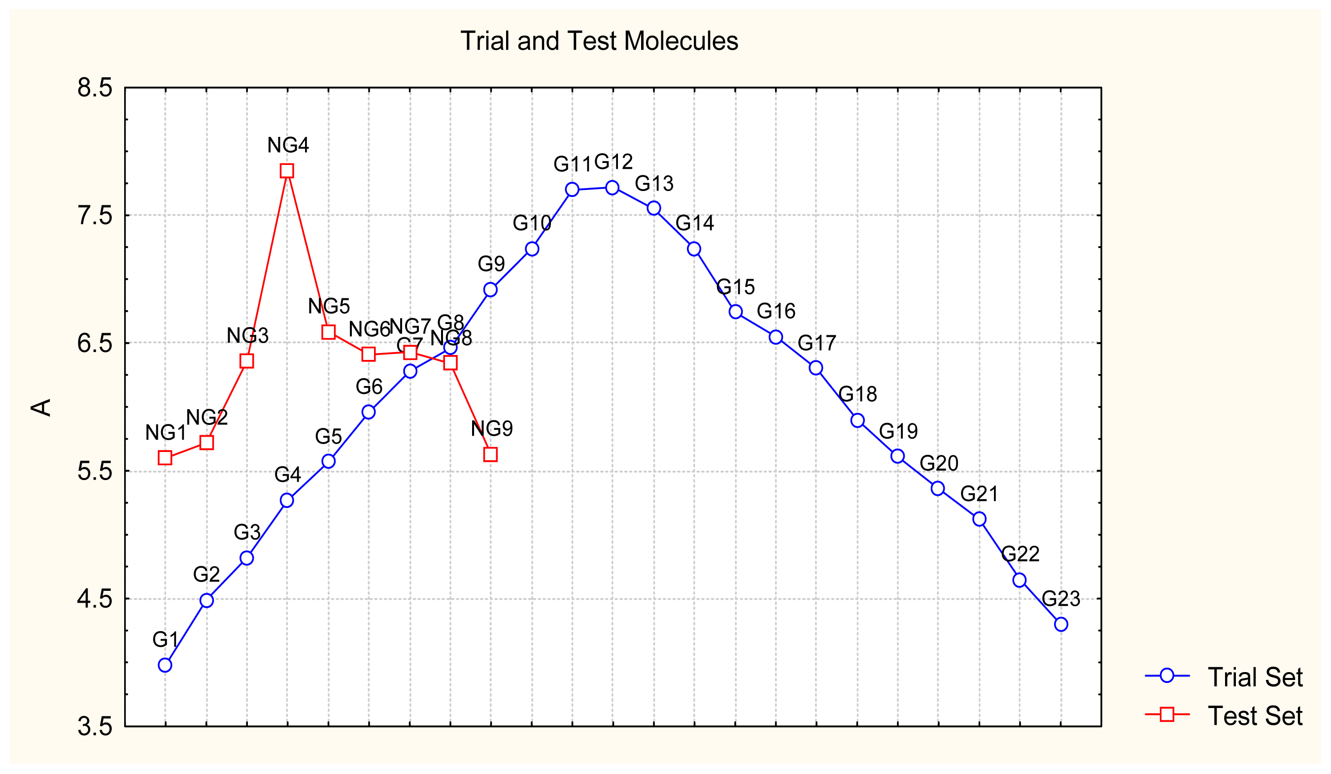
- Appropriate measures of goodness-of-fit, robustness and predictivity: The trial results were evaluated by external validation employing a testing set, which was selected by means of Gaussian vs. non-Gaussian distributions of the compounds’ activities, an improvement over the earlier arbitrariness of sampling the compounds only within a certain activity range. For instance, for linear QSAR the predicted correlation was superior to the tested correlation, thus confirming the reliability of this validation technique.
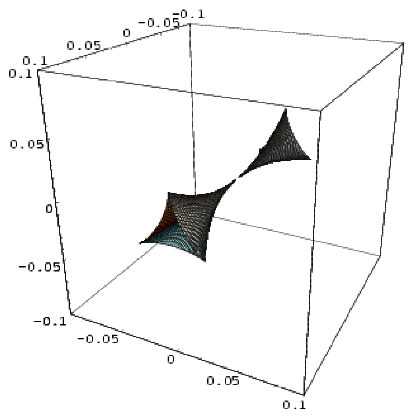
- A mechanistic interpretation: The selected succession of catastrophe-QSARs indicates that the inhibitor-HIV protein binding mutations that are involved in “birth and death” processes are associated with “waves” of induced activity in certain structural domain variants (see Figure 2). Moreover, the flat QSAR hypersurface should be complemented with catastrophe analysis to determine the specific structural domains for optimum interactions (see Figure 3) and for the associated molecular structure design of NNRT inhibitors.
Acknowledgements
Appendix
A1. More on Catastrophe Theory Background
A2. Catastrophe Theory Implication on Pearson Correlation
References
- Thom, R. Stabilitè Structurelle et Morphogènése; Benjamin-Addison-Wesley: New York, NY, USA, 1973. [Google Scholar]
- Viret, J. Reaction of the organism to stress: The survival attractor concept. Acta Biotheor 1994, 42, 99–109. [Google Scholar]
- Lacorre, P. Predation and generation processes through a new representation of the cusp catastrophe. Acta Biotheor 1997, 45, 93–115. [Google Scholar]
- Viret, J. Topological approach of Jungian psychology. Acta Biotheor 2010, 58, 233–245. [Google Scholar]
- Cerf, R. Catastrophe theory enables moves to be detected towards and away from self-organization: The example of epileptic seizure onset. Biol. Cybern 2006, 94, 459–468. [Google Scholar]
- Silvi, B.; Savin, A. Classification of chemical bonds based on topological analysis of electron localization functions. Nature 1994, 371, 683–686. [Google Scholar]
- Putz, M.V. Markovian approach of the electron localization functions. Int. J. Quantum Chem 2005, 105, 1–11. [Google Scholar]
- Aerts, D.; Czachor, M.; Gabora, L.; Kuna, M.; Posiewnik, A.; Pykacz, J.; Syty, M. Quantum morphogenesis: A variation on Thom’s catastrophe theory. Phys. Rev 2003, 67. [Google Scholar] [CrossRef]
- De Clercq, E. Anti-HIV drugs: 25 compounds approved within 25 years after the discovery of HIV. Int. J. Antimicrob. Agents 2009, 33, 307–320. [Google Scholar]
- De Clercq, E. The history of antiretrovirals: Key discoveries over the past 25 years. Rev. Med. Virol 2009, 19, 287–299. [Google Scholar]
- El Safadi, Y.; Vivet-Boudou, V.; Marquet, R. HIV-1 reverse transcriptase inhibitors. Appl. Microbiol. Biotechnol 2007, 75, 723–737. [Google Scholar]
- Ivetac, A; McCammon, J.A. Elucidating the inhibition mechanism of HIV-1 non-nucleoside reverse transcriptase inhibitors through multi-copy molecular dynamics simulations. J. Mol. Biol. 2009, 388, 644–658. [Google Scholar]
- Gupta, S.P. Advances in QSAR studies of HIV-1 reverse transcriptase inhibitors. Prog. Drug Res 2002, 58, 223–264. [Google Scholar]
- Prabhakar, Y.S.; Solomon, V.R.; Gupta, M.K.; Katti, S.B. QSAR studies on thiazolidines: A biologically privileged scaffold. Top. Heterocycl. Chem 2006, 4, 161–249. [Google Scholar]
- Prajapati, D.G.; Ramajayam, R.; Yadav, M.R.; Giridhar, R. The search for potent, small molecule NNRTIs: A review. Bioorg Med. Chem 2009, 17, 5744–5762. [Google Scholar]
- Zhan, P.; Chen, X.; Li, D.; Fang, Z.; de Clercq, E.; Liu, X. HIV-1 NNRTIs: Structural diversity, pharmacophore similarity, and implications for drug design. Med. Res. Rev 2011, in press. [Google Scholar]
- Chen, X.; Zhan, P.; Li, D.; De Clercq, E.; Liu, X. Recent advances in DAPYs and related analogues as HIV-1 NNRTIs. Curr. Med. Chem 2011, 18, 359–376. [Google Scholar]
- Rebehmed, J.; Barbault, F.; Teixeira, C.; Maurel, F. 2D and 3D QSAR studies of diarylpyrimidine HIV-1 reverse transcriptase inhibitors. J. Comput. Aided Mol. Des 2008, 22, 831–841. [Google Scholar]
- Afantitis, A.; Melagraki, G.; Sarimveis, H.; Koutentis, P.A.; Markopoulos, J.; Igglessi-Markopoulou, O. A novel simple QSAR model for the prediction of anti-HIV activity using multiple linear regression analysis. Mol. Divers 2006, 10, 405–414. [Google Scholar]
- Marino, D.J.G.; Castro, E.A.; Toropov, A. Improved QSAR modeling of anti-HIV-1 activities by means of the optimized correlation weights of local graphs invariants. Central Eur. J. Chem 2006, 4, 135–148. [Google Scholar]
- Mandal, A.S.; Roy, K. Predictive QSAR modeling of HIV reverse transcriptase inhibitor TIBO derivatives. Eur. J. Med. Chem 2009, 44, 1509–1524. [Google Scholar]
- Bak, A.; Polanski, J. A 4D-QSAR study on anti-HIV HEPT analogues. Bioorg. Med. Chem 2006, 14, 273–279. [Google Scholar]
- Duda-Seiman, C.; Duda-Seiman, D.; Dragoş, D.; Medeleanu, M.; Careja, V.; Putz, M.V.; Lacrămă, A.-M.; Chiriac, A.; Nuţiu, R.; Ciubotariu, D. Design of anti-HIV ligands by means of minimal topological difference (MTD) Method. Int. J. Mol. Sci 2006, 7, 537–555. [Google Scholar]
- Medina-Franco, J.L.; Rodríguez-Morales, S.; Juárez-Gordiano, C.; Hernández-Campos, A.; Castillo, R. Docking-based CoMFA and CoMSIA studies of non-nucleoside reverse transcriptase inhibitors of the pyridinone derivative type. J. Comput. Aided Mol. Des 2004, 18, 345–360. [Google Scholar]
- Topliss, J. Quantitative Structure-Activity Relationships of Drugs; Academic Press: New York, NY, USA, 1983. [Google Scholar]
- Seyfel, J.K. QSAR and Strategies in the Design of Bioactive Compounds; VCH Weinheim: New York, NY, USA, 1985. [Google Scholar]
- Duchowicz, P.R.; Castro, E.A. The Order Theory in QSPR-QSAR Studies; Mathematical Chemistry Monographs, University of Kragujevac: Kragujevac, Serbia, 2008. [Google Scholar]
- Zhao, V.H.; Cronin, M.T.D.; Dearden, J.C. Quantitative structure-activity relationships of chemicals acting by non-polar narcosis—Theoretical considerations. Quant. Struct. Act. Relat 1998, 17, 131–138. [Google Scholar]
- Pavan, M.; Netzeva, T.; Worth, A.P. Review of literature based quantitative structure-activity relationship models for bioconcentration. QSAR Comb. Sci 2008, 27, 21–31. [Google Scholar]
- Pavan, M.; Worth, A.P. Review of estimation models for biodegradation. QSAR Comb. Sci 2008, 27, 32–40. [Google Scholar]
- Putz, M.V.; Putz, A.M. Timisoara Spectral—Structure Activity Relationship (Spectral-SAR) Algorithm: From statistical and algebraic fundamentals to quantum consequences. In Quantum Frontiers of Atoms and Molecules; Putz, M.V., Ed.; NOVA Science Publishers Inc: New York, NY, USA, 2011; Volume Chapter 21, pp. 539–580. [Google Scholar]
- OECD Principles: Guidance Document on the Validation of (Q)SARModels; OECD Envioronment Diretorate: Paris, France, 2007.
- Putz, M.V.; Putz, A.M.; Barou, R. Spectral-SAR Realization of OECD-QSAR Principles. Int. J. Chem. Model 2011, 3. in press. [Google Scholar]
- Krokidis, X.; Noury, S.; Silvi, B. Characterization of elementary chemical processes by catastrophe theory. J. Phys. Chem. A 1997, 101, 7277–7282. [Google Scholar]
- Putz, M.V. Path integrals for electronic densities, reactivity indices, and localization functions in quantum systems. Int. J. Mol. Sci 2009, 10, 4816–4940. [Google Scholar]
- Weisstein, E.W. Catastrophe. From MathWorld—A Wolfram Web Resource. Available online: http://mathworld.wolfram.com/Catastrophe.html accessed on 1 September 2011.
- Sanns, W. Catastrophe Theory with Mathematica: A Geometric Approach; DAV: Waghäusel, Germany, 2000. [Google Scholar]
- Lu, X.-F.; Chen, Z.-W. The development of anti-HIV-1 drugs. Acta Pharm. Sin 2010, 45, 165–176. [Google Scholar]
- Putz, M.V. Residual-QSAR. Implications for genotoxic carcinogenesis. Chem. Central J 2011, 5. [Google Scholar] [CrossRef]
- Putz, M.V.; Lazea, M.; Sandjo, L.P. Quantitative Structure Inter-Activity Relationship (QSInAR). Cytotoxicity study of some hemisynthetic and isolated natural steroids and precursors on human fibrosarcoma cells HT1080. Molecules 2011, 16, 6603–6620. [Google Scholar]
- Putz, M.V.; Ionaşcu, C.; Putz, A.M.; Ostafe, V. Alert-QSAR. Implications for electrophilic theory of chemical carcinogenesis. Int. J. Mol. Sci 2011, 12, 5098–5134. [Google Scholar]
- Hypercube, Inc. HyperChem 7.01 [Program Package]; Hypercube, Inc: Gainesville, FL, USA, 2002. [Google Scholar]
- Leo, A.; Hansch, C.; Elkins, D. Partition coefficients and their uses. Chem. Rev 1971, 71, 525–616. [Google Scholar]
- Cronin, D.; Mark, T. The role of hydrophobicity in toxicity prediction. Curr. Comput. Aided Drug Design 2006, 2, 405–413. [Google Scholar]
- Selassie, C.D. History of Quantitative Structure-Activity Relationships. In Burger’s Medicinal Chemistry and Drug Discovery, 6th ed; Abraham, D.J., Ed.; Wiley: New York, NY, USA, 2003; pp. 1–48. [Google Scholar]
- Masterton, W.L.; Slowinski, E.J.; Stanitski, C.L. Chemical Principles; CBS College Publishing: Philadelphia, PA, USA, 1983. [Google Scholar]
- Chattaraj, P.K.; Sengupta, S. Popular electronic structure principles in a dynamical context. J. Phys. Chem 1996, 100, 16126–16130. [Google Scholar]
- Himmel, D.M.; Das, K.; Clark, A.D.; Hughes, S.H.; Benjahad, A.; Oumouch, S.; Guillemont, J.; Coupa, S.; Poncelet, A.; Csoka, I.; et al. Crystal structures for HIV-1 reverse transcriptase in complexes with three pyridinone derivatives: A new class of non-nucleoside inhibitors effective against a broad range of drug-resistant strains. J. Med. Chem 2005, 48, 7582–7591. [Google Scholar]
- The European Bioinformatics Institute. Available online: http://www.ebi.ac.uk/pdbsum/2BE2 accessed on 11 September 2011.
- Duda-Seiman, C.; Duda-Seiman, D.; Putz, M.V.; Ciubotariu, D. QSAR modeling of anti-HIV activity with HEPT derivatives. Digest J. Nanomat. Biostruct 2007, 2, 207–219. [Google Scholar]
- Croce, C.M. Oncogenes and cancer. N. Engl. J. Med 2008, 358, 502–511. [Google Scholar]
- Dingli, D.; Nowak, M.A. Cancer biology: Infectious tumour cells. Nature 2006, 443, 35–36. [Google Scholar]
- Benigni, R.; Bossa, C.; Jeliazkova, N.; Netzeva, T.; Worth, A. The Benigni/Bossa rules for mutagenicity and carcinogenicity—A module of Toxtree; European Commission report EUR 23241; Office for Official Publications of the European Communities: Luxembourg, 2008; pp. 1–69. [Google Scholar]
- Hansch, C.; Kurup, A.; Garg, R.; Gao, H. Chem-bioinformatics and QSAR: A review of QSAR lacking positive hydrophobic terms. Chem. Rev 2001, 101, 619–672. [Google Scholar]
- Putz, M.V.; Lacrămă, A.M. Introducing spectral structure activity relationship (S-SAR) analysis. Application to ecotoxicology. Int. J. Mol. Sci 2007, 8, 363–391. [Google Scholar]
- Putz, M.V.; Putz, A.M.; Lazea, M.; Chiriac, A. Spectral vs. statistic approach of structure-activity relationship. Application on ecotoxicity of aliphatic amines. J Theor. Comput. Chem 2009, 8, 1235–1251. [Google Scholar]
- QSAR & Spectral-SAR in Computational Ecotoxicology; Putz, M.V. (Ed.) Apple Academics: Ontario, Canada, 2012; in press.
- Zeeman, E.C. Catastrophe theory. Sci. Am 1976, 234, 65–83. [Google Scholar]
- Morse, M. The critical points of a functional on n variables. Trans. Am. Math. Soc 1931, 33, 72–91. [Google Scholar]
- Arnold, V.I. Local normal forms of functions. Invent. Math 1976, 35, 87–109. [Google Scholar]
- Poston, T.; Stewart, I. Catastrophe Theory and Its Applications; Pitman Publishing: Boston, MA, USA, 1978. [Google Scholar]
- Todeschini, R.; Consonni, V. Handbook of Molecular Descriptors; Wiley-VCH: Weinheim, Germany, 2000. [Google Scholar]


| Observed Activity | Structural | Predictor | Variables | ||
|---|---|---|---|---|---|
| A | X1 | … | Xk | … | XM |
| A1 | x11 | … | x1k | … | x1M |
| A2 | x21 | … | x2k | … | x2M |
| ⋮ | ⋮ | ⋮ | ⋮ | ⋮ | ⋮ |
| AN | xN1 | … | xNk | … | xNM |
| Name | Co-dimension | Co-rank | Universal unfolding | Parametric Representation |
|---|---|---|---|---|
| Fold | 1 | 1 | x3 + ux | 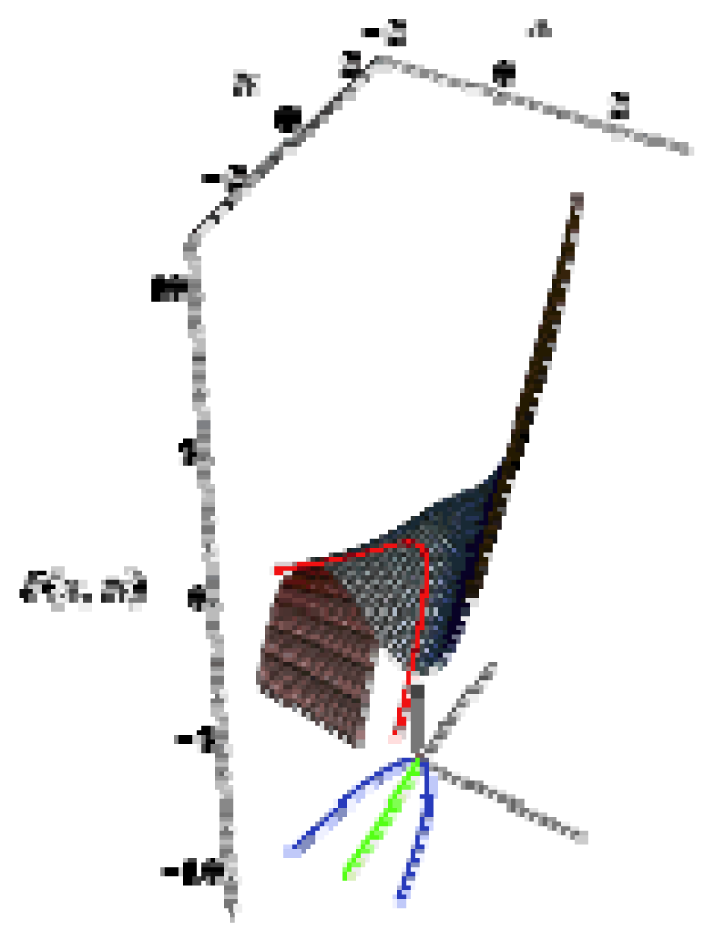 |
| Cusp | 2 | 1 | x4 + ux2 + vx |  |
| Swallow tail | 3 | 1 | x5 + ux3 + vx2 + wx | 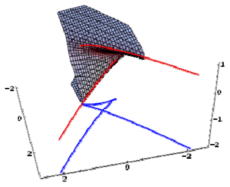 |
| Butterfly | 4 | 1 | x6 + ux4 + vx3 + wx2 + tx | 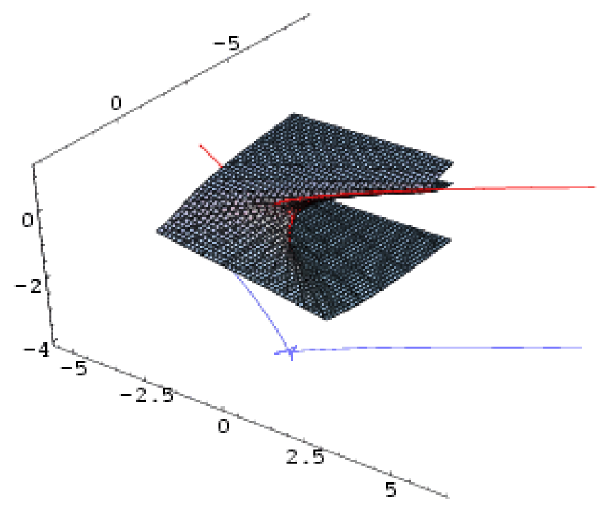 |
| Hyperbolic umbilic | 3 | 2 | x3 + y3 + uxy + vx + wy | 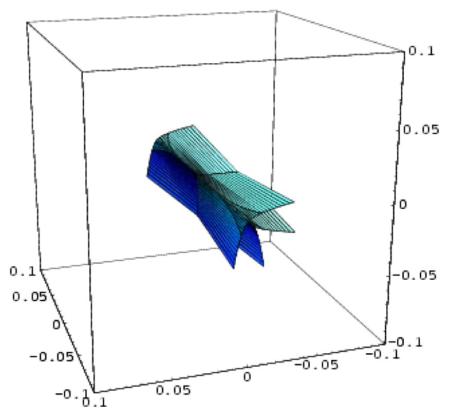 |
| Elliptic umbilic | 3 | 2 | x3 − xy2 + u(x2 + y2 ) + vx + wy |  |
| Parabolic umbilic | 4 | 2 | x2 y + y4 + ux2 + vy2 + wx + ty | 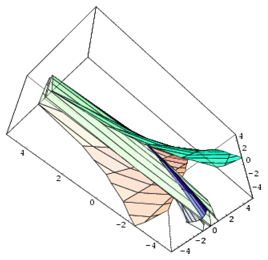 |
| Model | QSAR Equation |
|---|---|
| GROUP I: with one descriptor only, |X1〉 | |
| QSAR-(I) | |
| Fold | |
| Cusp | |
| Swallow tail | |
| Butterfly | |
| GROUP II: with two descriptors, |X1〉,|X2〉 | |
| QSAR- (II) | |
| Hyperbolic umbilic | |
| Elliptic umbilic | |
| Parabolic umbilic | |
| No. | Type | WORKING MOLECULES | Aobs | QSAR parameters | |||
|---|---|---|---|---|---|---|---|
| Structure | Name | Log (1/IC50) | Log P | POL (Å3) | H (kcal/mol) | ||
| 1. | G1 | 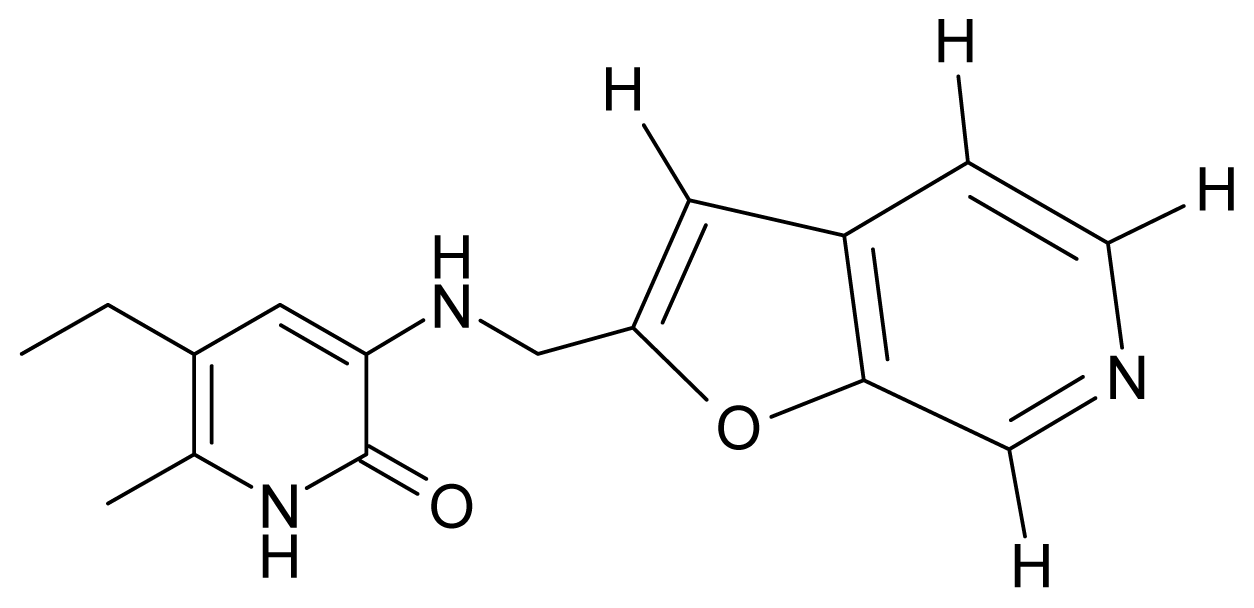 | 3-{[(6′-azabenzofuran-2′-yl) methyl]amino}-5-ethyl-6-methylpyridin-2(1H)-one | 3.98 | −0.54 | 31.21 | −14.67 |
| 2. | G2 | 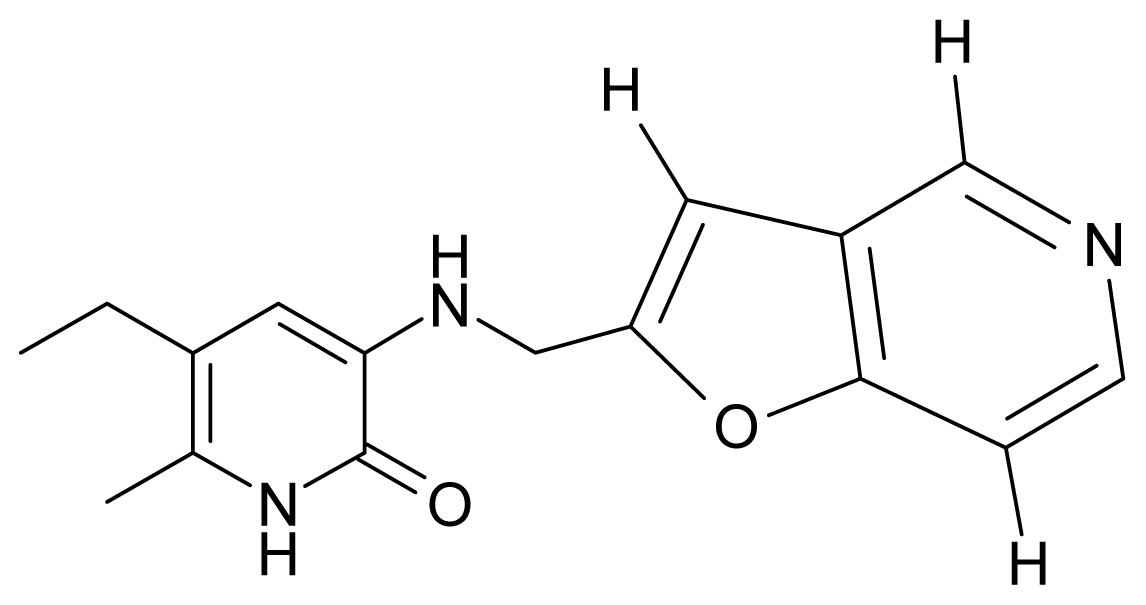 | 3-{[(5′-azabenzofuran-2′-yl) methyl]amino}-5-ethyl-6-methylpyridin-2(1H)-one | 4.49 | −0.54 | 31.21 | −16.195 |
| 3. | G3 | 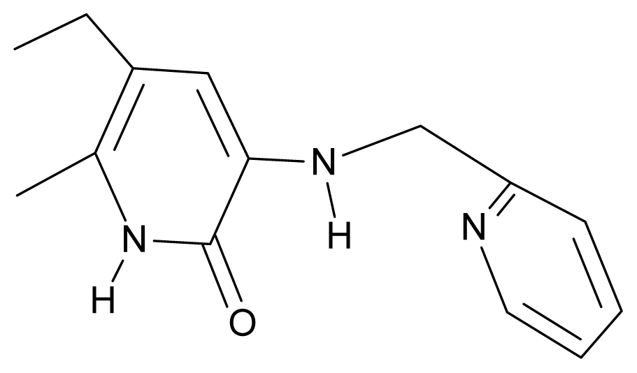 | 3-{[(pyridine-2′-yl) methyl]amino}-5-ethyl-6-methylpyridin-2(1H)-one | 4.82 | 0.21 | 27.87 | -5.854 |
| 4. | G4 | 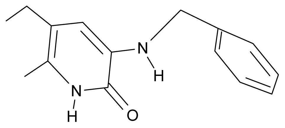 | 3-benzylamino-5-ethyl-6-methylpyridin-2(1H)-one | 5.27 | 0.67 | 28.58 | −11.659 |
| 5. | G5 | 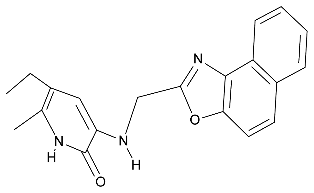 | 3-{[(1′,3′-naftoxazol-2′-yl) methyl]amino}-5-ethyl-6-methylpyridin-2(1H)-one | 5.57 | 1.20 | 38.48 | −1.878 |
| 6. | G6 | 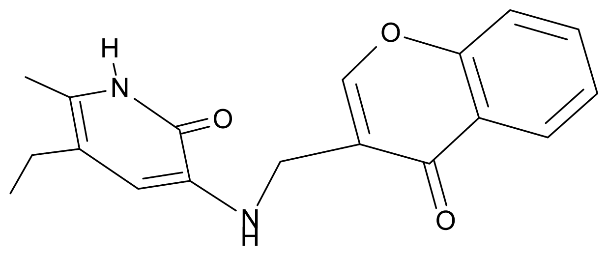 | 3-{[(1′-benzopyran-4′-one-3′-yl) methyl]amino}-5-ethyl-6-methylpyridin-2(1H)-one | 5.96 | −0.71 | 33.84 | −61.455 |
| 7. | G7 | 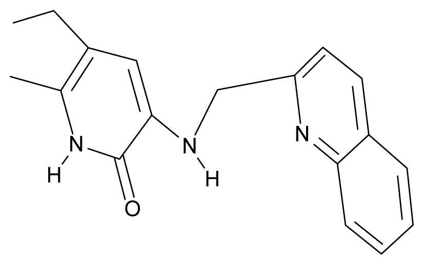 | 3-{[(benzopyridine-2′-yl) methyl]amino}-5-ethyl-6-methylpyridin-2(1H)-one | 6.28 | 1.16 | 35.14 | 11.246 |
| 8. | G8 | 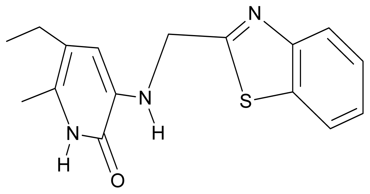 | 3-{[(1′,3′-benzothiazole-2′-yl) methyl]amino}-5-ethyl-6-methylpyridin-2(1H)-one | 6.46 | 0.54 | 33.57 | 17.808 |
| 9. | G9 | 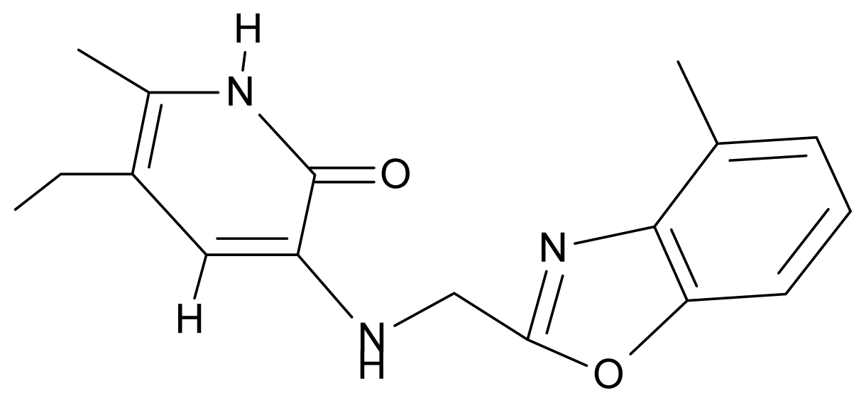 | 3-{[(4′-methylbenzoxazole-2′-yl) methyl]amino}-5-ethyl-6-methylpyridin-2(1H)-one | 6.92 | 0.67 | 33.05 | −27.613 |
| 10. | G10 | 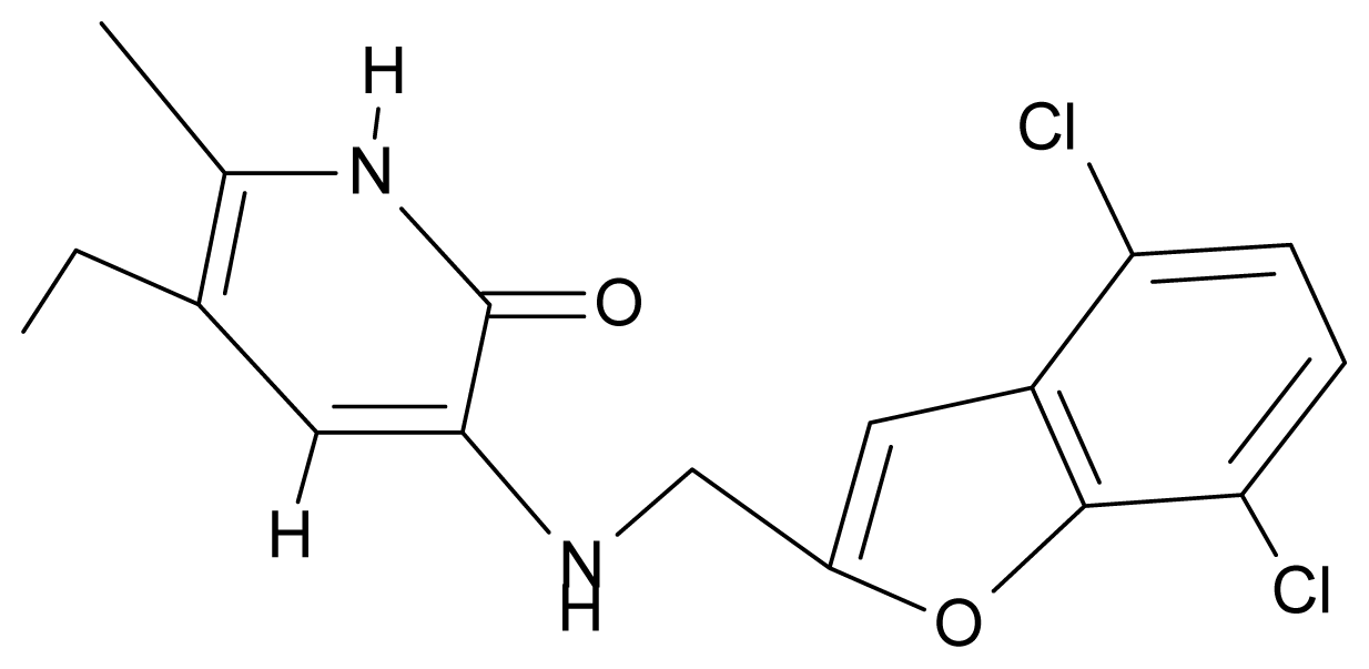 | 3-{[(4′,7′-dichlorobenzofuran-2′-yl) methyl]amino}-5-ethyl-6-methylpyridin-2(1H)-one | 7.24 | 0.88 | 35.78 | −33.749 |
| 11. | G11 | 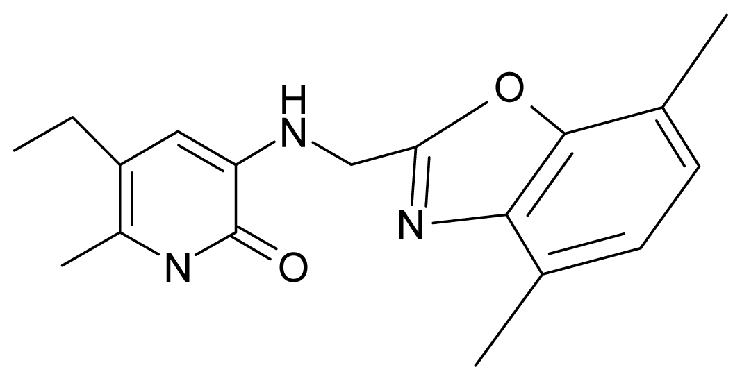 | 3-{[(4′,7′-dimethylbenzoxazol-2′-yl) methyl]amino}-5-ethyl-6-methylpyridin-2(1H)-one | 7.7 | 1.13 | 34.88 | −38.048 |
| 12. | G12 | 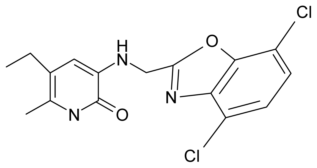 | 3-{[(4′,7′-dichlorobenzoxazol-2′-yl) methyl]amino}-5-ethyl-6-methylpyridin-2(1H)-one | 7.72 | 1.24 | 35.07 | −30.071 |
| 13. | G13 | 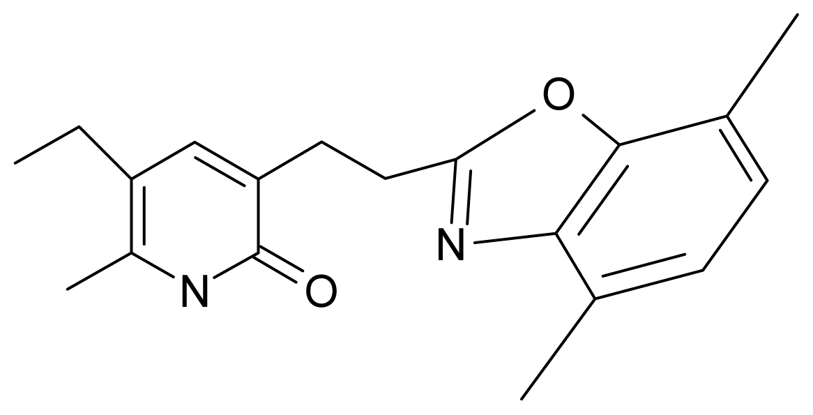 | 3-[(4′,7′-dimethylbenzoxazol-2′-yl) ethyl]-5-ethyl-6-methylpyridin-2(1H)-one | 7.55 | 2.62 | 35.37 | −47.701 |
| 14. | G14 | 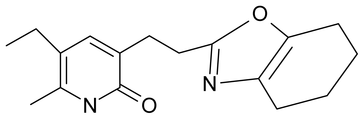 | 3-[(4′,5′,6′,7′-tetrahydrobenzoxazole-2′-yl) ethyl]-5-ethyl-6-methylpyridin-2(1H)-one | 7.24 | −0.02 | 32.08 | −63.299 |
| 15. | G15 | 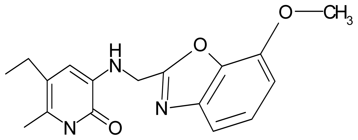 | 3-{[(4′-methoxybenzoxazole-2′-yl) methyl]amino}-5-ethyl-6-methylpyridin-2(1H)-one | 6.74 | −0.05 | 33.68 | −54.452 |
| 16. | G16 | 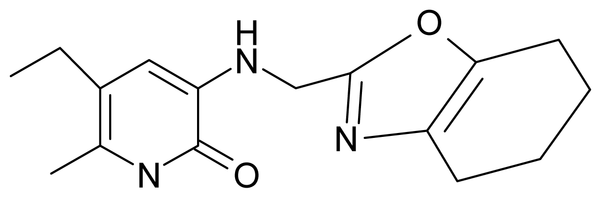 | 3-[(4′,5′,6′,7′-tetrahydrobenzoxazole-2′-yl) methyl]amino}-5-ethyl-6-methylpyridin-2(1H)-one | 6.55 | −1.50 | 31.59 | −50.643 |
| 17. | G17 | 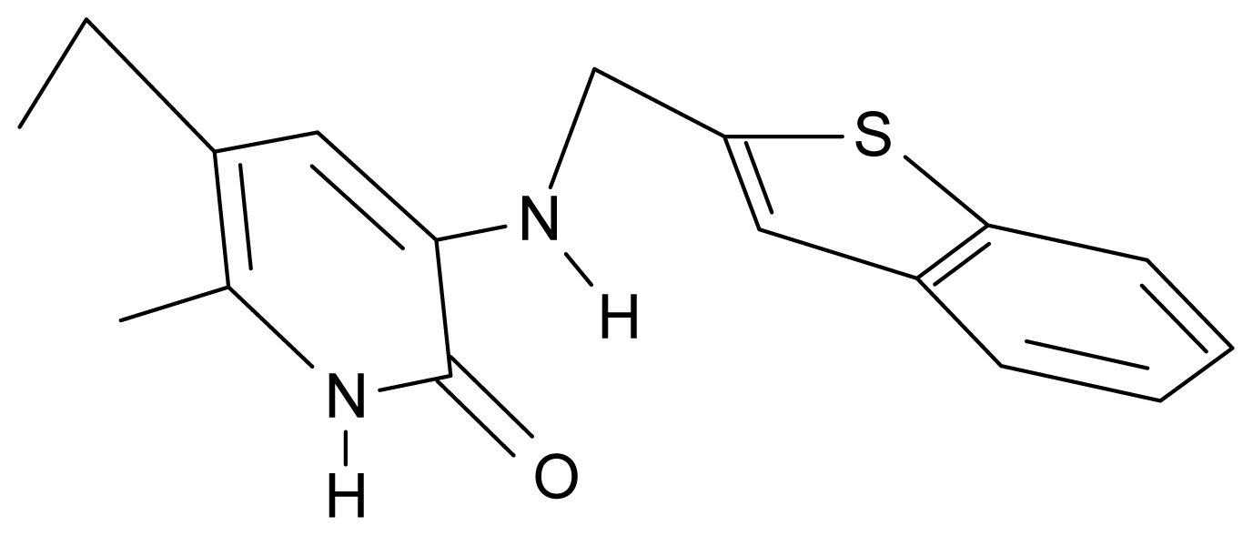 | 3-{[(benzothiophene-2′-yl) methyl] amino}-5-ethyl-6-methylpyridin-2(1H)-one | 6.30 | 0.19 | 34.28 | 11.703 |
| 18. | G18 | 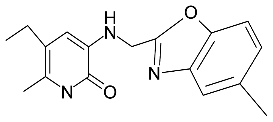 | 3-{[(5′-methylbenzoxazole-2′-yl) methyl]amino}-5-ethyl-6-methylpyridin-2(1H)-one | 5.90 | 0.67 | 33.05 | −27.741 |
| 19. | G19 | 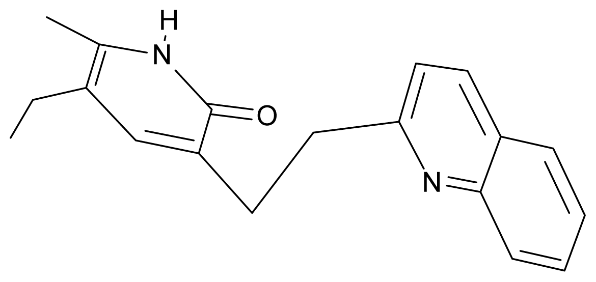 | 3-[(benzopyridine-2′-yl) ethyl]5-ethyl-6-methylpyridin-2(1H)-one | 5.61 | 2.71 | 35.62 | 3.331 |
| 20. | G20 | 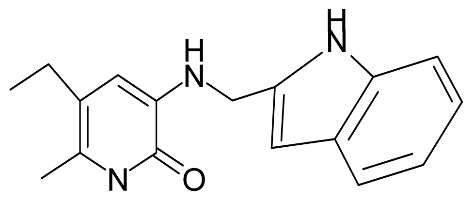 | 3-{[(indol-2′-yl) methyl] amino}-5-ethyl-6-methylpyridin-2(1H)-one | 5.36 | −0.34 | 32.63 | 4.727 |
| 21. | G21 |  | 3-{[(quinazolin-2′-yl) methyl]amino}-5-ethyl-6-methylpyridin-2(1H)-one | 5.12 | 0.02 | 31.92 | 8.171 |
| 22. | G22 | 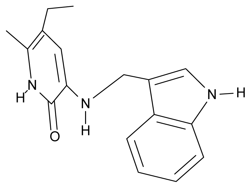 | 3-{[(indol-3′-yl)methyl] amino}-5-ethyl-6-methylpyridin-2(1H)-one | 4.65 | −0.43 | 32.63 | 2.957 |
| 23. | G23 | 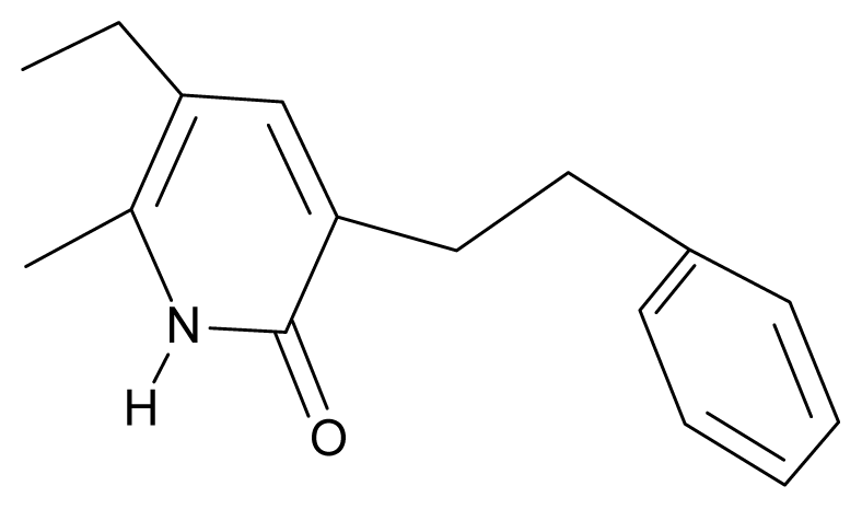 | 3-(β-phenilethyl)-5-ethyl-6-methylpyridin-2(1H)-one | 4.30 | 2.36 | 29.06 | −23.245 |
| 24. | NG1 | 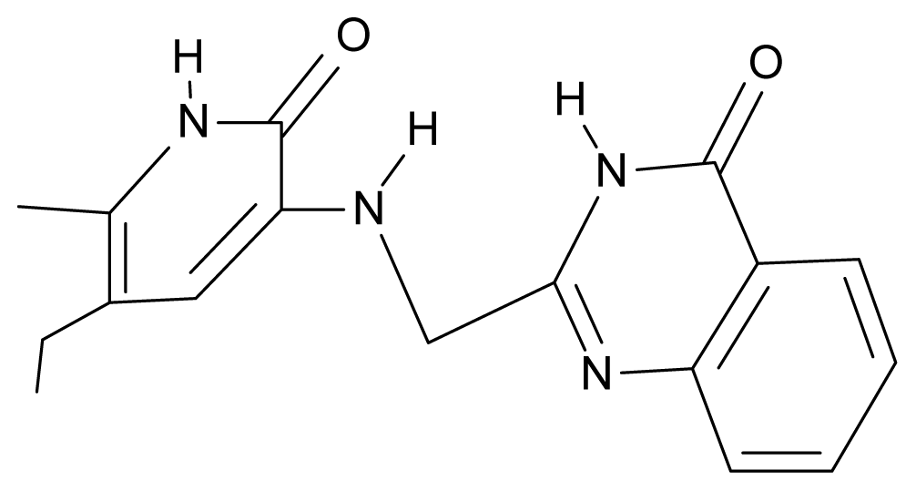 | 3-{[(4′-quinozolone-2′-yl) methyl]amino}-5-ethyl-6-methylpyridin-2(1H)-one | 5.60 | −0.47 | 33.85 | −36.959 |
| 25. | NG2 | 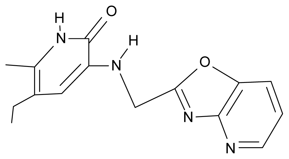 | 3-{[(3′,4′-diazobenzofuran-2′-yl) methyl]amino}-5-ethyl-6-methylpyridin-2(1H)-one | 5.72 | 0.05 | 30.50 | −8.120 |
| 26. | NG3 | 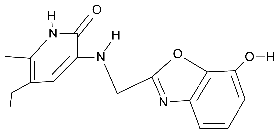 | 3-{[(7′-hydroxybenzoxazole-2′-yl) methyl]amino}-5-ethyl-6-methylpyridin-2(1H)-one | 6.36 | −0.08 | 31.85 | −62.189 |
| 27. | NG4 | 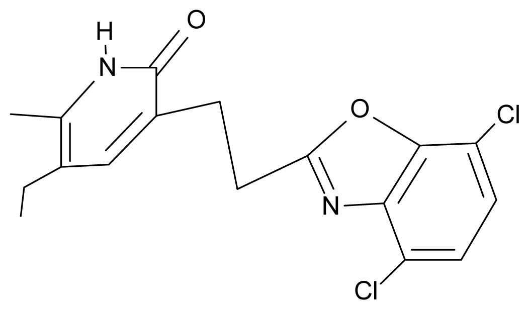 | 3-[(4′,7′-dichlorobenzoxazole-2′-yl) ethyl]-5-ethyl-6-methylpyridin-2(1H)-one | 7.85 | 2.72 | 35.55 | −39.459 |
| 28. | NG5 | 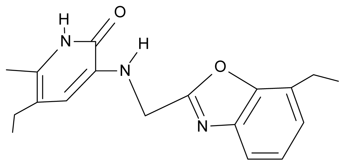 | 3-{[(7′-ethylbenzoxazole-2′-yl) methyl]amino}-5-ethyl-6-methylpyridin-2(1H)-one | 6.59 | 1.06 | 34.88 | −34.478 |
| 29. | NG6 | 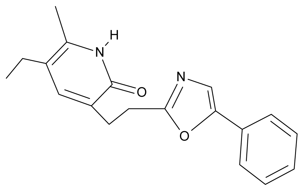 | 3-[(5′-phenyl-oxazole-2′-yl) ethyl]-5-ethyl-6-methylpyridin-2(1H)-one | 6.41 | 0.96 | 35.17 | −21.361 |
| 30. | NG7 | 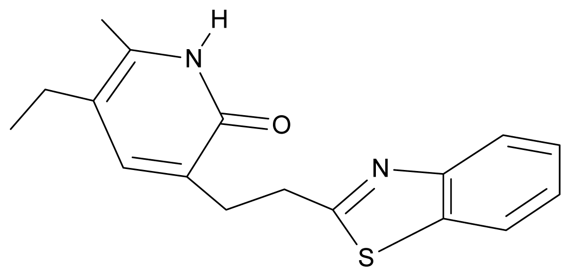 | 3-[(benzothiazole-2′-yl) ethyl]-5-ethyl-6-methylpyridin-2(1H)-one | 6.43 | 2.02 | 34.06 | 8.873 |
| 31. | NG8 | 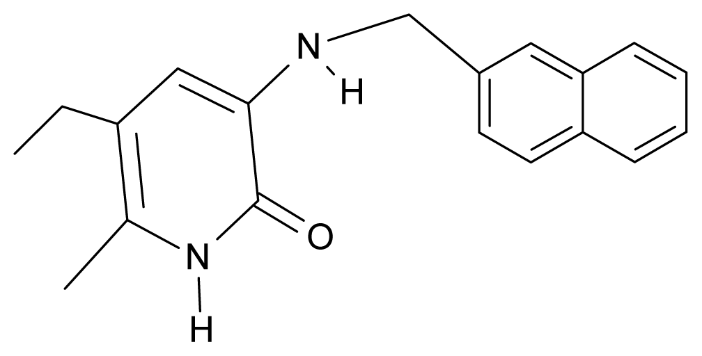 | 3-{[(2′naphtyl) methyl] amino}-5-ethyl-6-methylpyridin-2(1H)-one | 6.34 | 1.67 | 35.85 | 5.495 |
| 32. | NG9 | 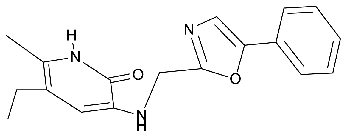 | 3-{[(5′-phenyl-oxazole-2′-yl) methyl]amino}-5-ethyl-6-methylpyridin-2(1H)-one | 5.63 | −0.53 | 34.69 | −10.850 |
| Catastrophe | QSAR Model | RPearson(a) | RALG(b) | r(c) | t-Stud. | t(d) | Fisher | f(e) | Π(f) |
|---|---|---|---|---|---|---|---|---|---|
| QSAR (I) | 0.228 | 0.984 | 4.317 | 22.344 | 7.854 | 1.150 | 0.143 | 8.963 | |
| 0.554 | 0.989 | 1.784 | −0.832 | −0.292 | 9.284 | 1.158 | 2.147 | ||
| 0.476 | 0.987 | 2.074 | 20.597 | 7.24 | 6.156 | 0.768 | 7.57 | ||
| Fold (F) | 0.382 | 0.986 | 2.581 | 22.936 | 8.062 | 1.705 | 0.213 | 8.468 | |
| 0.601 | 0.989 | 1.646 | −1.422 | −0.45 | 5.650 | 0.704 | 1.859 | ||
| 0.481 | 0.987 | 2.053 | 20.095 | 7.063 | 3.01 | 0.375 | 7.365 | ||
| Cusp (C) | 0.348 | 0.985 | 2.832 | 16.120 | 5.666 | 0.872 | 0.109 | 6.335 | |
| 0.713 | 0.992 | 1.391 | 2.240 | 0.787 | 6.558 | 0.818 | 1.796 | ||
| 0.764 | 0.993 | 1.300 | 19.802 | 6.960 | 8.864 | 1.105 | 7.166 | ||
| Swallow tail (ST) | 0.575 | 0.989 | 1.720 | 18.665 | 6.561 | 2.222 | 0.277 | 6.788 | |
| 0.715 | 0.992 | 1.387 | 0.45 | 0.158 | 4.708 | 0.587 | 1.515 | ||
| 0.763 | 0.993 | 1.302 | 15.608 | 5.486 | 6.263 | 0.781 | 5.692 | ||
| Butterfly (B) | 0.578 | 0.989 | 1.711 | 15.169 | 5.332 | 1.704 | 0.212 | 5.604 | |
| 0.718 | 0.992 | 1.382 | −0.355 | −0.125 | 3.619 | 0.451 | 1.459 | ||
| 0.856 | 0.996 | 1.163 | 19.088 | 6.709 | 9.349 | 1.166 | 6.908 |
| Catastrophe | QSAR Model | RPearson(a) | RALG(b) | r(c) | t-Stud. | t(d) | Fisher | f(e) | Π(f) |
|---|---|---|---|---|---|---|---|---|---|
| QSAR (II) | 0.556 | 0.989 | 1.778 | −0.702 | −0.245 | 4.464 | 0.763 | 1.9504 | |
| 0.556 | 0.989 | 1.778 | 18.564 | 6.489 | 4.468 | 0.764 | 6.771 | ||
| 0.728 | 0.992 | 1.363 | −1.151 | −0.402 | 11.302 | 1.932 | 2.398 | ||
| Hyperbolic umbilic (HU) | 0.715 | 0.992 | 1.387 | −2.215 | −0.774 | 3.561 | 0.609 | 1.701 | |
| 0.736 | 0.992 | 1.3485 | 19.328 | 6.756 | 4.019 | 0.687 | 6.923 | ||
| 0.755 | 0.993 | 1.315 | −0.79 | −0.276 | 4.503 | 0.770 | 1.549 | ||
| Elliptic umbilic (EU) | 0.757 | 0.993 | 1.312 | −2.548 | −0.891 | 3.582 | 0.612 | 1.670 | |
| 0.722 | 0.992 | 1.374 | 1.866 | 0.652 | 2.908 | 0.497 | 1.600 | ||
| 0.843 | 0.995 | 1.181 | 20.638 | 7.214 | 6.542 | 1.118 | 7.395 | ||
| Elliptic umbilic (EU) | 0.851 | 0.995 | 1.170 | 17.047 | 5.958 | 7.015 | 1.199 | 6.189 | |
| 0.857 | 0.996 | 1.162 | 3.124 | 1.092 | 7.346 | 1.256 | 2.029 | ||
| 0.853 | 0.996 | 1.167 | 0.532 | 0.186 | 7.120 | 1.217 | 1.696 | ||
| Parabolic umbilic (PU) | 0.722 | 0.992 | 1.374 | 1.817 | 0.635 | 2.905 | 0.497 | 1.593 | |
| 0.703 | 0.992 | 1.411 | −2.219 | −0.776 | 2.611 | 0.446 | 1.671 | ||
| Parabolic umbilic (PU) | 0.874 | 0.996 | 1.140 | 20.243 | 7.075 | 8.645 | 1.478 | 7.317 | |
| 0.767 | 0.993 | 1.295 | 16.828 | 5.882 | 3.815 | 0.652 | 6.058 | ||
| 0.841 | 0.995 | 1.183 | 0.386 | 0.135 | 6.447 | 1.102 | 1.623 | ||
| 0.856 | 0.996 | 1.163 | 3.074 | 1.074 | 7.292 | 1.246 | 2.015 |
| Log P | F | C | ST | B |
|---|---|---|---|---|
| QSAR | 1.750 | 2.645 | 2.905 | 3.627 |
| F | 2.411 | 1.732 | 2.865 | |
| C | 1.437 | 1.174 | ||
| ST | 1.231 |
| POL | F | C | ST | B |
|---|---|---|---|---|
| QSAR | 0.517 | 1.198 | 0.828 | 0.830 |
| F | 1.317 | 0.717 | 0.524 | |
| C | 0.670 | 0.983 | ||
| ST | 0.314 |
| H | F | C | ST | B |
|---|---|---|---|---|
| QSAR | 0.431 | 0.89 | 1.916 | 1.127 |
| F | 1.054 | 1.793 | 1.242 | |
| C | 1.509 | 0.292 | ||
| ST | 1.29 |
| |Log P ÷ POL| | F | C | ST | B |
|---|---|---|---|---|
| QSAR | 1.233 | 1.446 | 2.076 | 2.797 |
| F | 1.094 | 1.015 | 2.341 | |
| C | 0.767 | 0.191 | ||
| ST | 0.917 |
| |Log P ÷ H| | F | C | ST | B |
|---|---|---|---|---|
| QSAR | 1.32 | 1.755 | 0.988 | 2.501 |
| F | 1.358 | 0.062 | 1.624 | |
| C | 0.072 | 0.882 | ||
| ST | 0.059 |
| |POL ÷ H| | F | C | ST | B |
|---|---|---|---|---|
| QSAR | 0.086 | 0.309 | 1.088 | 0.297 |
| F | 0.264 | 1.076 | 0.717 | |
| C | 0.839 | 0.691 | ||
| ST | 0.976 |
| Log P^POL | HU | EU | PU |
|---|---|---|---|
| QSAR | 0.675 | 0.810 | 1.005 |
| HU | 0.139 | 1.414 | |
| EU | 1.531 |
| Log P^H | HU | EU | PU |
|---|---|---|---|
| QSAR | 0.512 | 0.917 | 1.123 |
| HU | 0.964 | 0.878 | |
| EU | 1.152 |
| POL^H | HU | EU | PU |
|---|---|---|---|
| QSAR | 1.170 | 1.652 | 1.640 |
| HU | 1.46 | 1.440 | |
| EU | 0.02 |
| Model | ||||||
|---|---|---|---|---|---|---|
| Molecule | ||||||
| NG1 | 5.586 | 6.179 | 5.294 | 5.094 | −20.595 | 5.687 |
| NG2 | 5.729 | 4.885 | 4.294 | 5.719 | −9.764 | 4.360 |
| NG3 | 5.676 | 0.415 | 4.708 | 5.531 | −13.457 | −7.932 |
| NG4 | 5.729 | 6.156 | 5.149 | 6.657 | −29.709 | 5.259 |
| NG5 | 6.487 | 6.141 | 5.309 | 6.705 | −25.700 | 5.923 |
| NG6 | 6.399 | 5.438 | 5.258 | 6.708 | −27.365 | 5.219 |
| NG7 | 6.903 | 5.631 | 5.319 | 5.311 | −21.540 | 5.984 |
| NG8 | 6.904 | 5.334 | 5.027 | 5.995 | −31.693 | 5.566 |
| NG9 | 5.580 | 4.9357 | 5.328 | 5.054 | −24.666 | 4.383 |
| R-Pearson | 0.195 | 0.129 | 0.174 | 0.701 | 0.488 | 0.026 |
| Model | ||||||
|---|---|---|---|---|---|---|
| Molecule | ||||||
| NG1 | 6.0865 | 5.918 | 5.308 | 5.387 | 5.351 | 7.210 |
| NG2 | 5.581 | 5.839 | 5.399 | 5.448 | 4.816 | 4.578 |
| NG3 | 6.785 | 6.132 | 7.526 | 5.686 | 1.423 | 7.234 |
| NG4 | 7.115 | 6.642 | 6.037 | 6.289 | 5.480 | 7.765 |
| NG5 | 6.495 | 7.382 | 6.853 | 7.277 | 6.033 | 7.629 |
| NG6 | 6.163 | 7.291 | 6.426 | 7.104 | 7.338 | 7.647 |
| NG7 | 5.790 | 7.388 | 6.087 | 7.615 | 6.879 | 6.547 |
| NG8 | 5.761 | 7.560 | 6.330 | 7.640 | 7.895 | 7.447 |
| NG9 | 5.467 | 5.755 | 4.786 | 5.177 | 7.586 | 7.303 |
| R-Pearson | 0.778 | 0.468 | 0.454 | 0.431 | 0.057 | 0.451 |
© 2011 by the authors; licensee MDPI, Basel, Switzerland. This article is an open-access article distributed under the terms and conditions of the Creative Commons Attribution license (http://creativecommons.org/licenses/by/3.0/).
Share and Cite
Putz, M.V.; Lazea, M.; Putz, A.-M.; Duda-Seiman, C. Introducing Catastrophe-QSAR. Application on Modeling Molecular Mechanisms of Pyridinone Derivative-Type HIV Non-Nucleoside Reverse Transcriptase Inhibitors. Int. J. Mol. Sci. 2011, 12, 9533-9569. https://doi.org/10.3390/ijms12129533
Putz MV, Lazea M, Putz A-M, Duda-Seiman C. Introducing Catastrophe-QSAR. Application on Modeling Molecular Mechanisms of Pyridinone Derivative-Type HIV Non-Nucleoside Reverse Transcriptase Inhibitors. International Journal of Molecular Sciences. 2011; 12(12):9533-9569. https://doi.org/10.3390/ijms12129533
Chicago/Turabian StylePutz, Mihai V., Marius Lazea, Ana-Maria Putz, and Corina Duda-Seiman. 2011. "Introducing Catastrophe-QSAR. Application on Modeling Molecular Mechanisms of Pyridinone Derivative-Type HIV Non-Nucleoside Reverse Transcriptase Inhibitors" International Journal of Molecular Sciences 12, no. 12: 9533-9569. https://doi.org/10.3390/ijms12129533