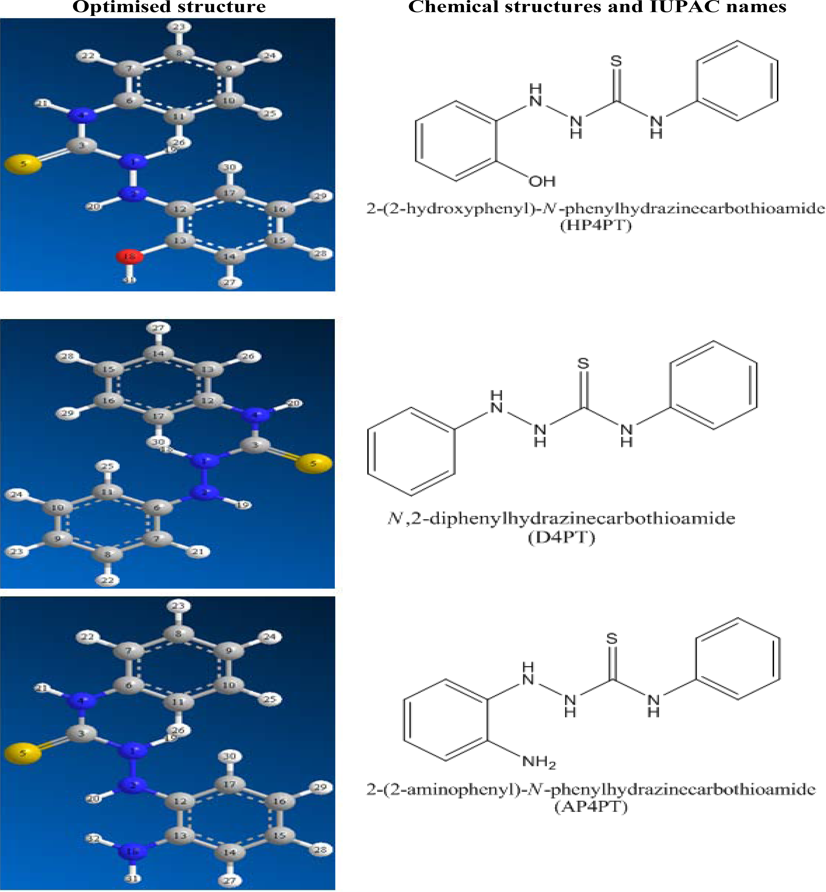
Figure 1 shows the chemical and optimized structures of the inhibitors (AP4PT, HP4PT and D4PT). Table 1 shows the corrosion rates and the % inhibition efficiencies of AP4PT, HP4PT and D4PT in acid media. The corrosion rate of mild steel for the blank solution (1 M H₂SO₄) is higher than those obtained for solutions containing various concentrations of AP4PT, HP4PT and D4PT. This indicates that the corrosion of mild steel in H₂SO₄ solution is inhibited by various concentrations of AP4PT, HP4PT and D4PT. It was also found that the corrosion rate of mild steel decreases with increase in the concentration of the inhibitor, but decreases with increasing temperature, which indicates that the inhibitory potentials of AP4PT, HP4PT and D4PT for mild steel corrosion increase with increasing concentration but decrease with increase in temperature. The values of % inhibition efficiencies obtained from the hydrogen evolution method are close to that obtained using the weight loss method (Table 1). From the calculated values of the inhibition efficiencies of AP4PT, HP4PT and D4PT, it is indicative that these inhibitors are adsorption inhibitors and that their inhibition efficiencies decrease in the following trend, AP4PT > HP4PT > D4PT. Furthermore, from the observed trend for the variation of inhibition efficiency with temperature, it is evident that the mechanism of adsorption of the inhibitors on mild steel surface is by a physical adsorption mechanism. For physical adsorption, the inhibition efficiency is expected to decrease with increasing temperature, but for chemical adsorption, the inhibition efficiency is expected to increase with increasing temperature [25].

The activation energies for the corrosion of mild steel in the absence and presence of the inhibitors were calculated using the logarithmic form of the Arrhenius Equation shown below [25]: (1) log C R 2 C R 1 = E a 2.303 R ( 1 T 1 − 1 T 2 )where CR₁ and CR₂ are the corrosion rates of mild steel at the temperatures T₁ (303 K) and T₂ (333 K), respectively. E_a is the activation energy for the reaction and R is the molar gas constant. Values of the E_a calculated from Equation 1 are presented in Table 2. The activation energies obtained for the inhibited corrosion of mild steel are within the limit expected (<80 KJ/mol) for the mechanism of physical adsorption, hence the adsorption of AP4PT, HP4PT and D4PT on mild steel surface is consistent with the mechanism of charge transfer from the inhibitor to the metal surface [26].

The heats of adsorption of AP4PT, HP4PT and D4PT on mild steel surface were calculated using the following Equation [25]: (2) Q a d s = 2.303 R [ log ( θ 2 1 − θ 2 ) − log ( θ 1 1 − θ 1 ) ] x ( T 1 X T 2 T 2 − T 1 ) k J m o l − 1where Q_ads is the heat of adsorption, R is the gas constant, θ₁ and θ₂ are the degrees of surface coverage of the inhibitors at the temperatures T₁ (303 K) and T₂ (333 K), respectively. Calculated values of Q_ads are negative, indicating that the adsorption of the inhibitors on the mild steel surface is exothermic (see Table 2).

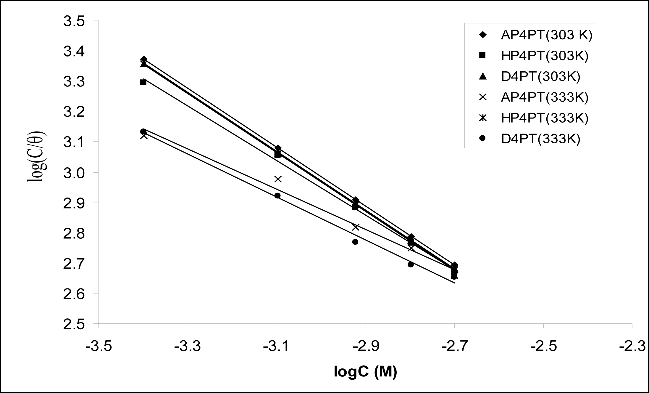
The adsorption characteristics of the inhibitors were investigated by fitting the experimental data obtained for the degrees of surface coverage into different adsorption isotherms. The tests revealed that the adsorption of AP4PT, HP4PT and D4PT can best be described by the Langmuir adsorption isotherm. The Equation for the Langmuir adsorption isotherm can be written as follows [27,28]: (3) θ =   K C   ×   1 / 1   +   K C )where K designates the adsorption equilibrium constant and C is the concentration of the inhibitor in the bulk electrolyte. From the rearrangement of Equation 3, Equations 4 and 5 are obtained.

Figure 2 shows the plots of values of log(C/θ) versus logC. The plots were found to be linear indicating the application of the Langmuir isotherm to the adsorption of AP4PT, HP4PT and D4PT on mild steel surface. Values of adsorption parameters deduced from the Langmuir adsorption isotherms are presented in Table 3. The results obtained indicated that the slopes and R² values were very close to unity, which signifies strong adherence of AP4PT, HP4PT and D4PT to the adsorption of the Langmuir model.

The values of the adsorption equilibrium constant (K) obtained from the intercept of the Langmuir adsorption isotherms are related to the free energy of adsorption according to Equation 6 [28,29]; (6) Δ G a d s 0 = − 2.303 R T   log ( 55.5 K )where ΔG⁰_ads is the free energy of adsorption, R is the gas constant and T is the temperature of the system. Calculated values of the free energies are also presented in Table 3. The free energies ranged from −10.51 to −16.76 kJ/mol and are within the range expected for the transfer of charge from the inhibitor to the metal surface. Therefore, the adsorption of AP4PT, HP4PT and D4PT is spontaneous. Generally, values of ΔG⁰_ads up to −20 kJ/mol signify physisorption, the inhibition acts due to electrostatic interactions between the charged molecules and the charged metal, while values around −40 kJ/mol or less are associated with chemisorption as a result of sharing or transfer of electrons from the organic molecules to the metal surface to form a coordinate type of bond (chemisorption). The values obtained from this study ranged from −10.51 to −16.76 kJ/mol, which support the mechanism of physical adsorption [30].

Quantum chemical calculations have been widely used to study reaction mechanisms [31]. They have also been proved to be a very powerful tool for studying inhibition of the corrosion of metals [32–34]. It has been found that the effectiveness of a corrosion inhibitor can be related to its electronic and spatial molecular structure [35–39]. In this study, the relationship between quantum chemical parameters and inhibition efficiency was investigated.

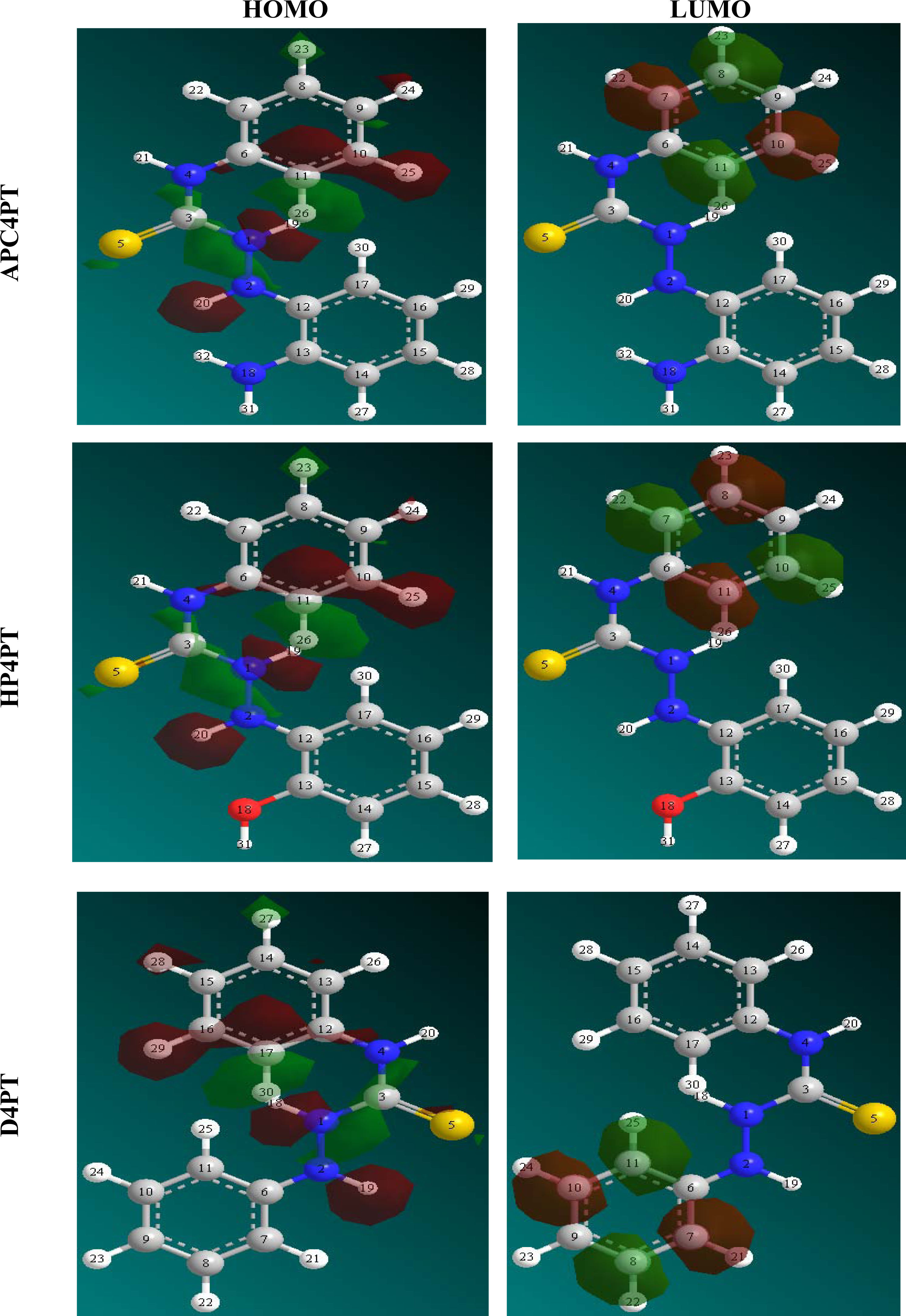
Table 4 shows the values of some quantum chemical parameters, namely the energy of the highest occupied molecular orbital (E_HOMO), energy of the lowest unoccupied molecular orbital (E_LUMO), the energy gap (E_LUMO-HOMO), the total electronic energy of the molecules (EE), core core repulsion (CC), dipole moment (μ), logP (substituent constant - measure of the differential solubility of a compound in two solvents and characterizes the hydrophobicity/hydrophilicity of a molecule), molecular polarizability (pol), cosmo volume (molecular volume) (cosVol) and cosmo area (molecular surface area or solvent accessible molecular surface area) (cosAr). The quantum chemical parameters were computed for five different Hamiltonians, namely, parametric method 6 (PM6), parametric method 3 (PM3), Austin model 1 (AM1), Recife model 1 (RM1) and modified neglect of diatomic overlap (MNDO) [40]. The results obtained from semi empirical computations, are presented in Table 4. As can be seen from Table 4, the E_HOMO, E_LUMO, ΔE and dipole moment values calculated for AP4PT by PM3 method heavily deviate from the data obtained from other Hamiltonians. This can be explained as follows. All the semi empirical methods contain sets of parameters. Atomic and diatomic parameters exist in PM6, while MNDO, AM1, PM3, and MNDO-d use only single-atom parameters. Not all parameters are optimized for all methods; for example, in MNDO and AM1 the two electron one center integrals are normally taken from atomic spectra. Therefore, in AP4PT, atomic and diatomic parameters are very significant. The frontier molecular orbital energies (i.e., E_HOMO and E_LUMO) are significant parameters for the prediction of the reactivity of a chemical species. The E_HOMO is often associated with the electron donating ability of a molecule [36–38]. Therefore, increasing values of E_HOMO indicates higher tendency for the donation of electron(s) to the appropriate acceptor molecule with low energy and empty molecular orbital. According to Eddy and Ebenso [40], increasing values of E_HOMO facilitate the adsorption of the inhibitor. Consequently, the inhibition efficiency of the inhibitor would be enhanced by improving the transport process through the adsorbed layer. From Table 4, it is evident that the E_HOMO for the inhibitors decreases in the order; (AP4PT > HP4PT > D4PT), which is consistent with the experimental % inhibition efficiency results. However, the E_LUMO decreases in a similar order. This can be explained as follows. The E_LUMO indicates the ability of the molecule to accept electrons. Therefore, the lower the value of E_LUMO the more apparent it is that the molecule would accept electrons. Also, the E_LUMO-HOMO (energy gap) was also found to decrease in the order similar to that of the E_LUMO. Literature reveals that a larger value of the energy gap indicates low reactivity to a chemical species because the energy gap is related to the softness or hardness of a molecule. A soft molecule is more reactive than a hard molecule because a hard molecule has a larger energy gap [37,38].

Values of logP (substituent constant) were also found to have a good relationship with the corrosion inhibition efficiencies of the studied inhibitors. Substituent constants are empirical quantities, which account for the variation of the structure and do not depend on the parent structure but vary with the substituent [39]. According to Eddy and Ebenso [40], logP accounts for the hydrophobicity of an actual molecule. Hydrophobicity of an organic molecule increases with decreasing water solubility. In corrosion studies, hydrophobicity is related to the mechanism of formation of the oxide/hydroxide layer on the metal surface (which reduces the corrosion process drastically). From the results obtained, based on the increasing value of logP, the inhibition efficiencies of the studied thiosemicarbazides increase in the following order, AP4PT > HP4PT > D4PT, which is consistent with experimental obtained % inhibition efficiency results.

The dipole moment (μ) is an index that can also be used for the prediction of the direction of a corrosion inhibition process. Dipole moment is the measure of polarity in a bond and is related to the distribution of electrons in a molecule [41]. Although literature is inconsistent on the use of ‘μ’ as a predictor for the direction of a corrosion inhibition reaction, it is generally agreed that the adsorption of polar compounds possessing high dipole moments on the metal surface should lead to better inhibition efficiency. Comparison of the results obtained from quantum chemical calculations with experimental inhibition efficiencies indicated that the % inhibition efficiencies of the inhibitors increase with increasing value of the dipole moment.

El Ashry et al. [42] noted that core core repulsion energy is a quantum chemical parameter that may have excellent correlation with inhibition efficiency. They reported that the inhibition efficiency of some Schiff bases decreased with increasing value of core core repulsion energy. Similarly, the inhibition efficiencies of the studied thiosemicarbazides were found to decrease with increasing values of core core repulsion. This study on quantum chemical descriptors has been extended to include the total and the electronic energies of the molecules. From the results, it is evident that based on the decreasing values of the total energy (TE) and electronic energy (EE), as well as decreasing value of cosmo area and cosmo volume, the trend for the variation of the inhibition efficiency follows the order similar to experimental %inhibition efficiencies (AP4PT > HP4PT > D4PT).

Polarizability is the ratio of induced dipole moment to the intensity of the electric field. The induced dipole moment is proportional to polarizability [43]. Some attempts have been made to relate the polarizability of some corrosion inhibitors to their inhibition efficiency. According to Arslan et al. [38], the minimum polarizability principle (MPP) expects that the natural direction of evolution of any system is towards a state of minimum polarizability. From the results obtained from quantum chemical calculations, the trend for the increase in the inhibition efficiencies of the inhibitors with respect to increasing polarizability correlates well with the order of the experimental % inhibition efficiencies results (AP4PT > HP4PT > D4PT).

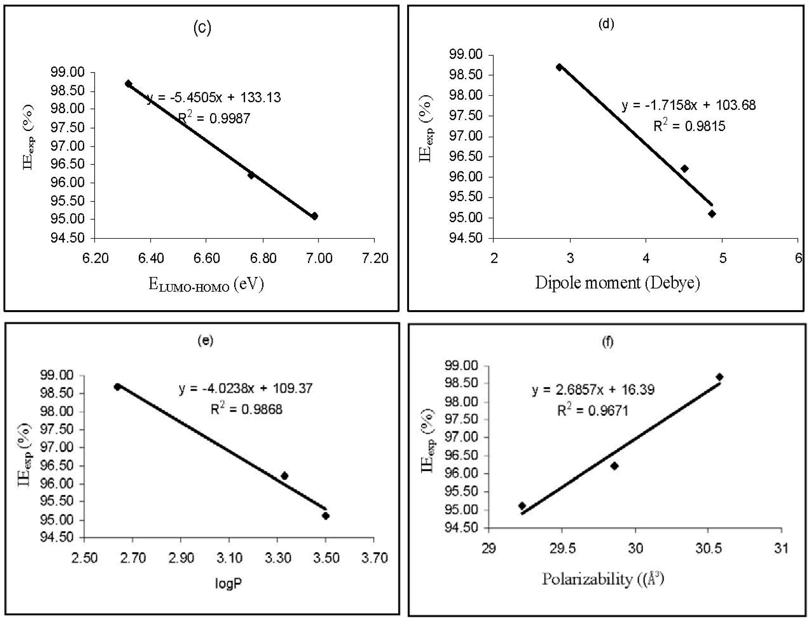
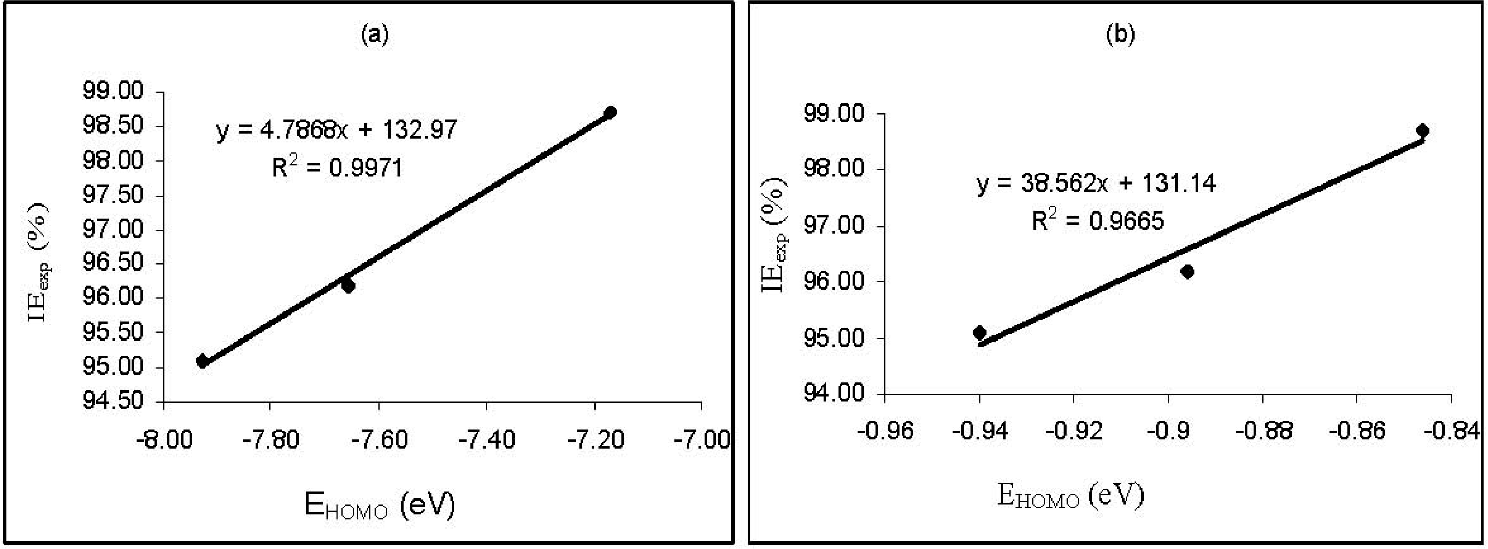
Correlations between the calculated quantum chemical parameters were also carried out. Figure 3 shows plots for the variation of the experimental inhibition efficiencies with some quantum chemical parameters. The figure reveals that the degree of linearity (R²) between the plotted quantum chemical parameters and the experimental inhibition efficiencies were very close to unity, which indicated a high degree of linearity. However, the plots were developed from parameters obtained from PM6 Hamiltonians. R² values for other Hamiltonians are presented in Table 5. From the results obtained, the highest degree of linearity between the experimental inhibition efficiencies and the E_HOMO, E_LUMO, E_LUMO-HOMO and μ were obtained from the AM1, PM6, AM1 and MNDO Hamiltonians, respectively. However, R² values with respect to EE, CC, cosVol and cosAr were relatively low.

According to Karelson and Lobanov [44], quantitative structure-activity and structure property relationship studies are unquestionably of great importance in modern chemistry and biochemistry. The concept of QSAR/QSPR is to transform searches for compounds with desired properties using chemical intuition and experience into mathematically quantified and computed form. Once a correlation between structure and activity/property is found, any number of compounds, including those not yet synthesized, can readily be screened on the computer [45,46].

Most recent studies on the use of QSPR/QSAR for corrosion employ quantum chemical calculations as an attractive source of new molecular descriptor. According to Vera et al. [47], QSAR/QSPR can be used to relate the inhibition efficiency of most inhibitors to structural parameters (quantum and topological), which can be theoretically calculated with the ultimate aim of obtaining a molecular design of new corrosion inhibitors. El Ashry et al. [48] also stated that although the QSAR is a useful tool for the development of new corrosion inhibitors, the development of Equations for calculating the corrosion inhibition efficiency may lead to a prediction of the efficiency of some inhibitors.

Attempts were made to establish the relationship between corrosion inhibition efficiencies and the calculated quantum chemical parameters using linear regression analysis. The linear model approximated the inhibition efficiency (IE_Theor) according to the following Equation [49]: (7) I E Theor = A x i C i + Bwhere A and B are the regression coefficients determined by regression analysis, x_i is a quantum chemical index characteristic of the molecule i, C_i is the experimental concentration of the inhibitor. Equation 7 did not give a good correlation between the experimental and theoretical inhibition efficiencies therefore, a non linear model, which was first proposed by Lukovits et al. [50] for the study of interaction of corrosion inhibitors with metal surface in acidic solutions, was used. This model is based on the Langmuir adsorption isotherm (which assumes that the coverage of the metal surface by the inhibitor’s molecule is the primary cause of corrosion inhibition) and can be written as follows [38]: (8) I E Theor ( % ) = ( A x j + B ) C i 1 + ( A x j + B ) C i ×   100

Using the non linear model, multiple regressions were performed between the inhibition efficiencies of the inhibitors and some quantum chemical parameters/descriptors. The solutions of the above non linear Equation are given by Equations 9 to 13 for PM6, PM3, AM1, RM1 and MNDO, respectively. The corresponding correlation coefficients (r) were 0.821, 0.8589, 0.7500, 0.8155 and 0.8068, respectively. Values of inhibition efficiencies calculated from Equations 9 to 13 are presented in Table 6.

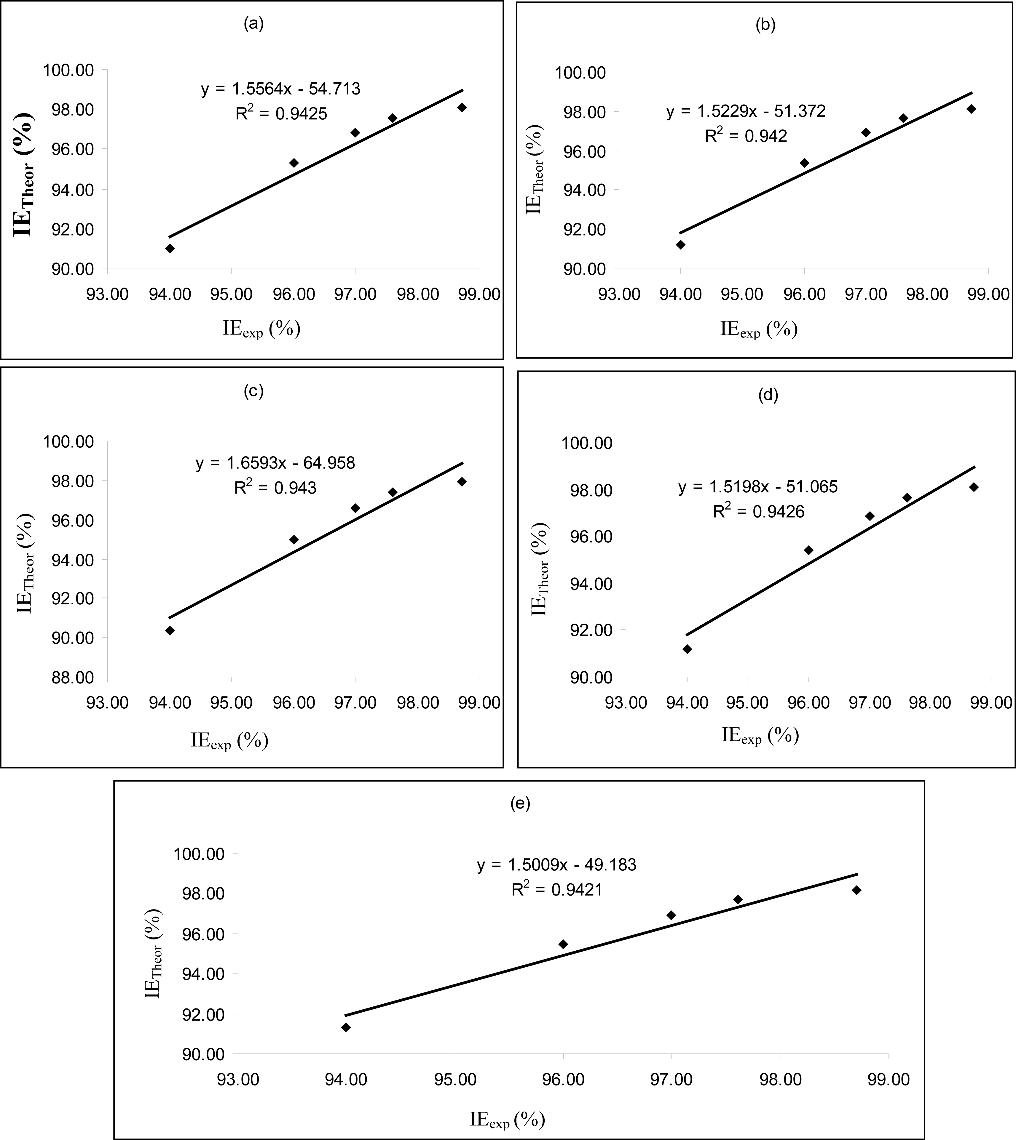
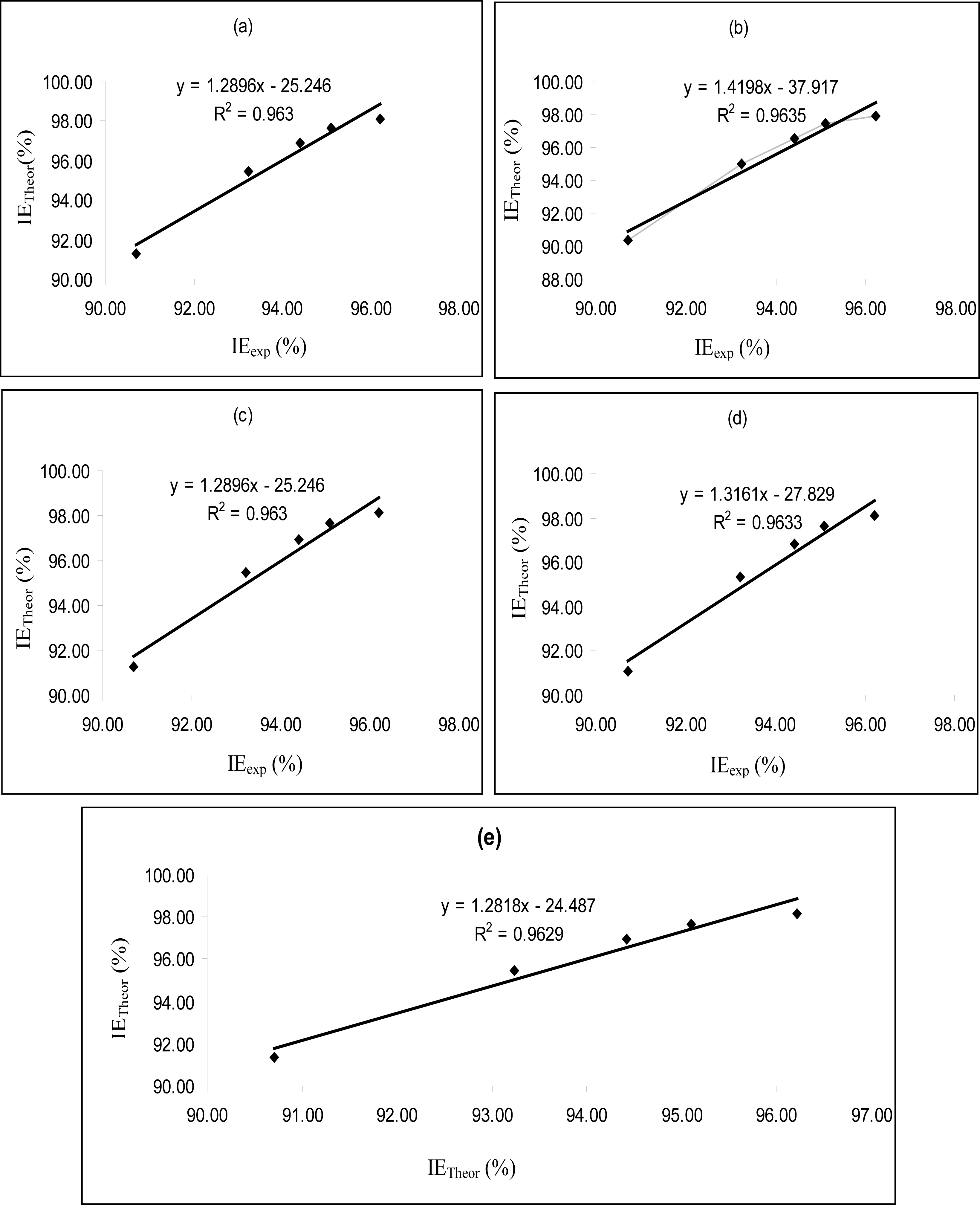
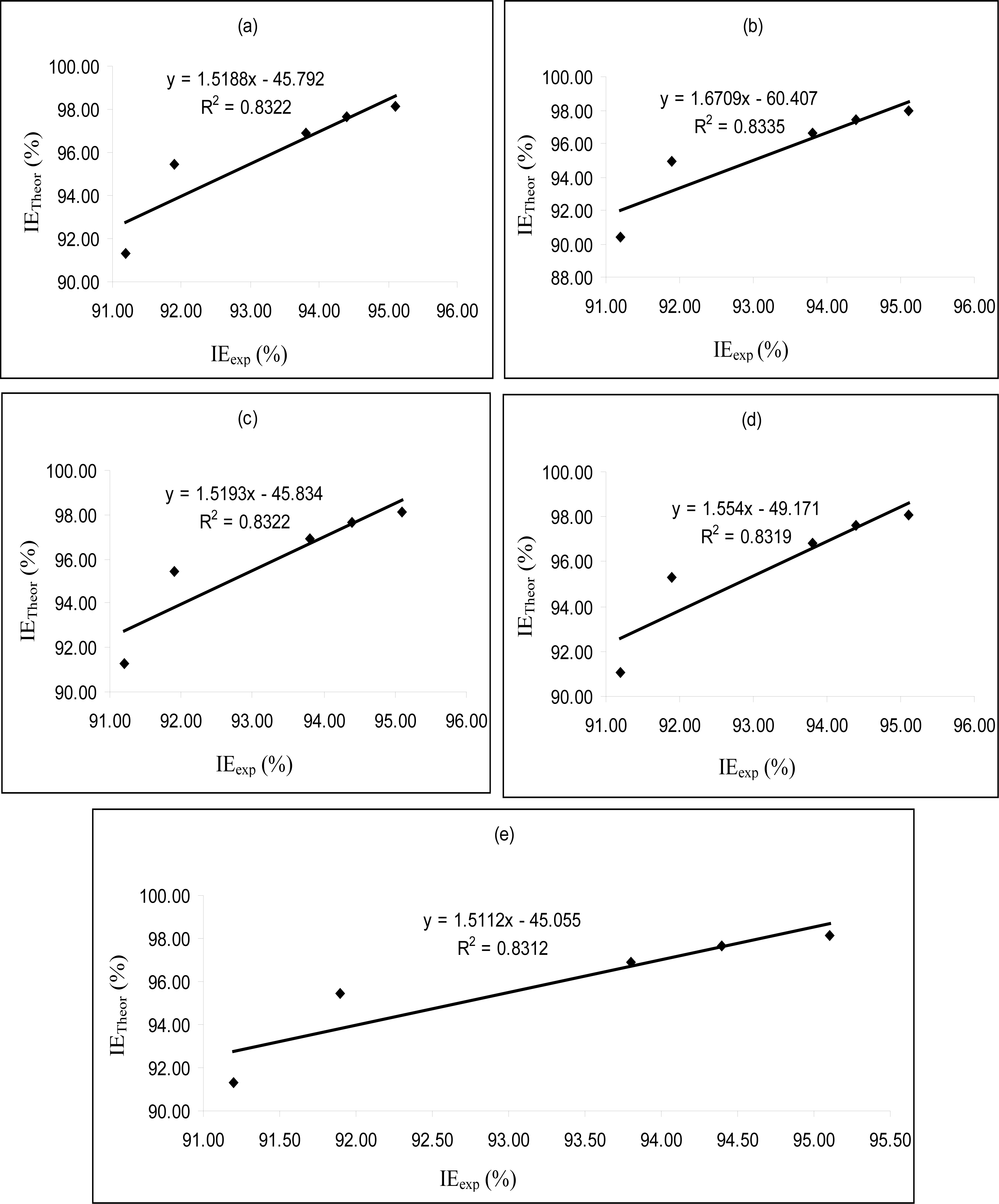
Figures 4–6 are plots showing the variation of experimental inhibition efficiencies with theoretical inhibition efficiencies for AP4PT, HP4PT and D4PT, respectively. From the plots, it is evident that there is a strong relationship between the theoretical and experimental inhibition efficiencies, indicating that these models can be used to predict the inhibition efficiencies of new corrosion inhibitors that are structurally related to the studied thiosemicarbazides.

DFT is based on solving the time independent Schrodinger Equation for the electrons of molecular systems as a function of the positions of the nuclei [51]. The premise behind the density functional theory is that the energy of a molecule can be determined from the electron density instead of a wave function [52]. However, in this study, MP2 method (Moller-Plesset perturbation theory method at level 2) was adopted for computation because of the bulkiness of the studied inhibitors.

Materials used for the study were mild steel sheets of composition (wt %); Mn (0.6), P (0.36), C (0.15) and Si (0.03) and the rest Fe. Each sheet was mechanically pressed cut to form different coupons, each of dimension 5 × 4 × 0.11 cm. Each coupon was degreased by washing with ethanol, dipped in acetone and allowed to air dry before they were preserved in a desiccator. All reagents used for the study were Analar grade and double distilled water was used for their preparation. The inhibitors 2-(2-aminophenyl) Nphenylhydrazinecarbothioamide(AP4PT),N,2diphenylhydrazinecarbothioamide(D4PT) and 2-(2-hydroxyphenyl)- phenylhydrazinecarbothioamide(HP4PT) were synthesized as described earlier by Kittur and Mahajan Shetti [55]. The concentrations of inhibitor used for the study was 4 × 10⁻⁴ to 20 × 10⁻⁴ M in 1L solution of 1M H₂SO₄.

In the gravimetric experiment, a previously weighed mild steel coupon was completely immersed in 250 mL of the test solution in an open beaker. The beaker was inserted into a water bath maintained at 303 K. After every 24 h, each sample was withdrawn from the test solution, washed in a solution containing 50% NaOH and 100 g/L of zinc dust. The washed coupons were dipped in acetone and allowed to air dry before re-weighing. The difference in weight for a period of 168 h (7 days) was taken as total weight loss. The experiments were repeated at 333 K. From the weight loss results, the inhibition efficiency (%I) of the inhibitor, degree of surface coverage and corrosion rates were calculated using Equations 26, 27, and 28. respectively [56]; (26) % IE = ( 1 − W 1 / W 2 ) × 100 (27) θ = 1 − W 1 / W 2 (28) C R ( gh − 1 cm − 2 ) = W / A twhere W₁ and W₂ are the weight losses (g) for mild steel in the presence and absence of the inhibitor in H₂SO₄ solution, θ is the degree of surface coverage of the inhibitor, A is the area of the mild steel coupon (in cm²), t is the period of immersion (in hours) and W is the weight loss of mild steel after time, t. All the measurements were performed in triplicate and the mean value recorded.

The hydrogen evolution technique (gasometric) experiment was carried out at 303 K as described in literature [56]. From the volume of hydrogen evolved per minute, inhibition efficiencies were calculated using Equation 29 below. (29) % IE = ( 1 − V H t 1 V H t o ) x 100where V H t 1 and V H t o are the volumes of H₂ gas evolved at time ‘t’ for inhibited and uninhibited solutions, respectively.

Single point energy calculations were carried out using AM1, PM6, PM3, MNDO and RM1 Hamiltonian in the MOPAC 2008 software for Windows [57]. Calculations were performed on an IBM compatible Intel Pentium IV (2.8 GHz, 4 GB RAM) computer. The following quantum chemical parameters were calculated: the energy of the highest occupied molecular orbital (E_HOMO), the energy of the lowest unoccupied molecular orbital (E_LUMO), the dipole moment (μ), the total energy (TE), the electronic energy (EE), the ionization potential, the cosmo area (cosAr) and the cosmo volume (cosVol). The polarizability (Pol) and logP were also calculated using Hyperchem release 8.0.3 for windows [58]. The Mulliken and Lowdin charges (q) for nucleophilic and electrophilic attacks were computed using GAMES computational software [59]. The correlation type and method used for the calculation was MP2 while the basis set was set to STO3G*.

Statistical analyses were performed using SPSS program version 15.0 for Windows. Non-linear regression analyses were performed by unconstrained sum of squared residuals for loss function and estimation methods of Levenberg-Marquardt using SPSS program version 15.0 for Windows [60].