Additive SMILES-Based Carcinogenicity Models: Probabilistic Principles in the Search for Robust Predictions

Abstract
:
1. Introduction
2. Materials and Methods
- DCWi:=0.5*CWi; Eps:=0.1*DCWi;
- Calculation of TF1; CWi:=CWi + DCWi;
- Calculation of TF2, after modify CWi;
- If TF2 > TF1 then TF1:=TF2; go to 2
- CWi:=CWi - DCWi;
- DCWi:= −0.5*DCWi;
- If absolute value (DCWi) >Eps then go to 2.
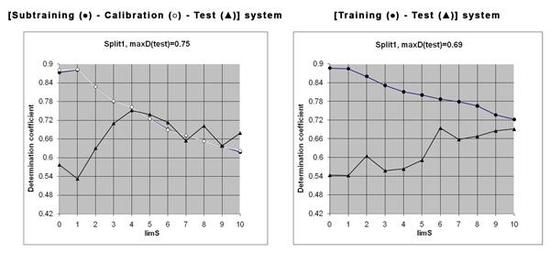
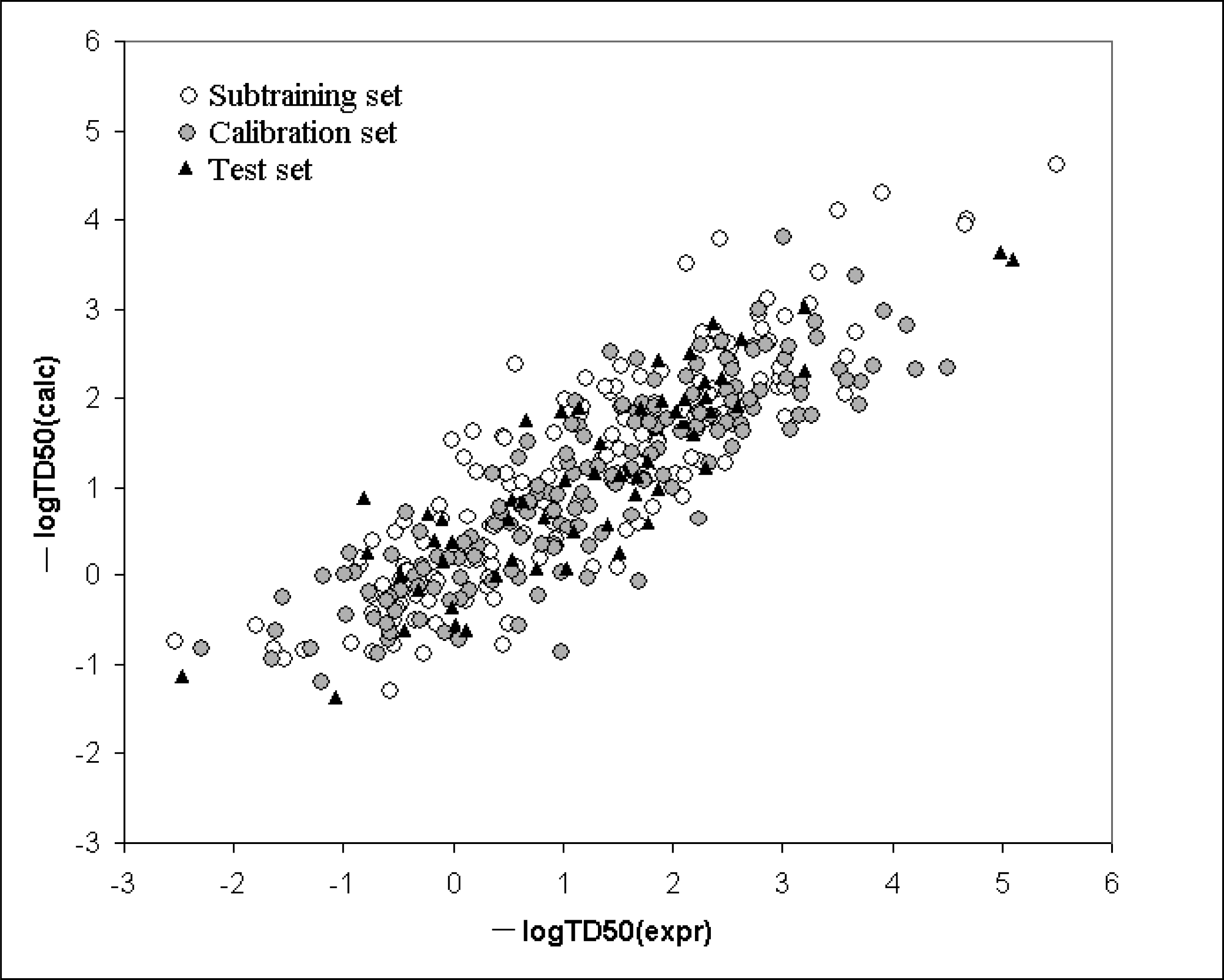
3. Results
- n=165, r2=0.7622, s=0.685, F=522 (subtraining set)
- n=167, r2=0.7620, s=0.734, F=528 (calibration set)
- n=61, r2=0.7541, s=0.682, F=181 (test set)
4. Discussion
5. Conclusions
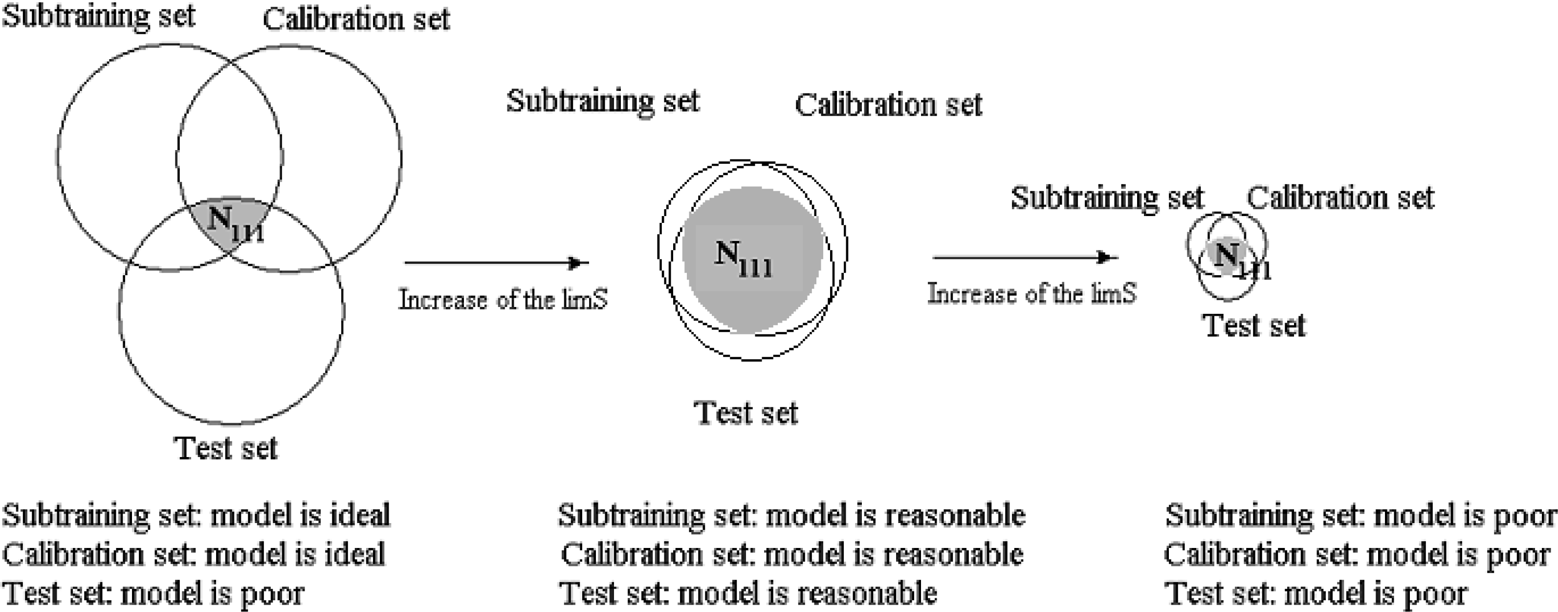
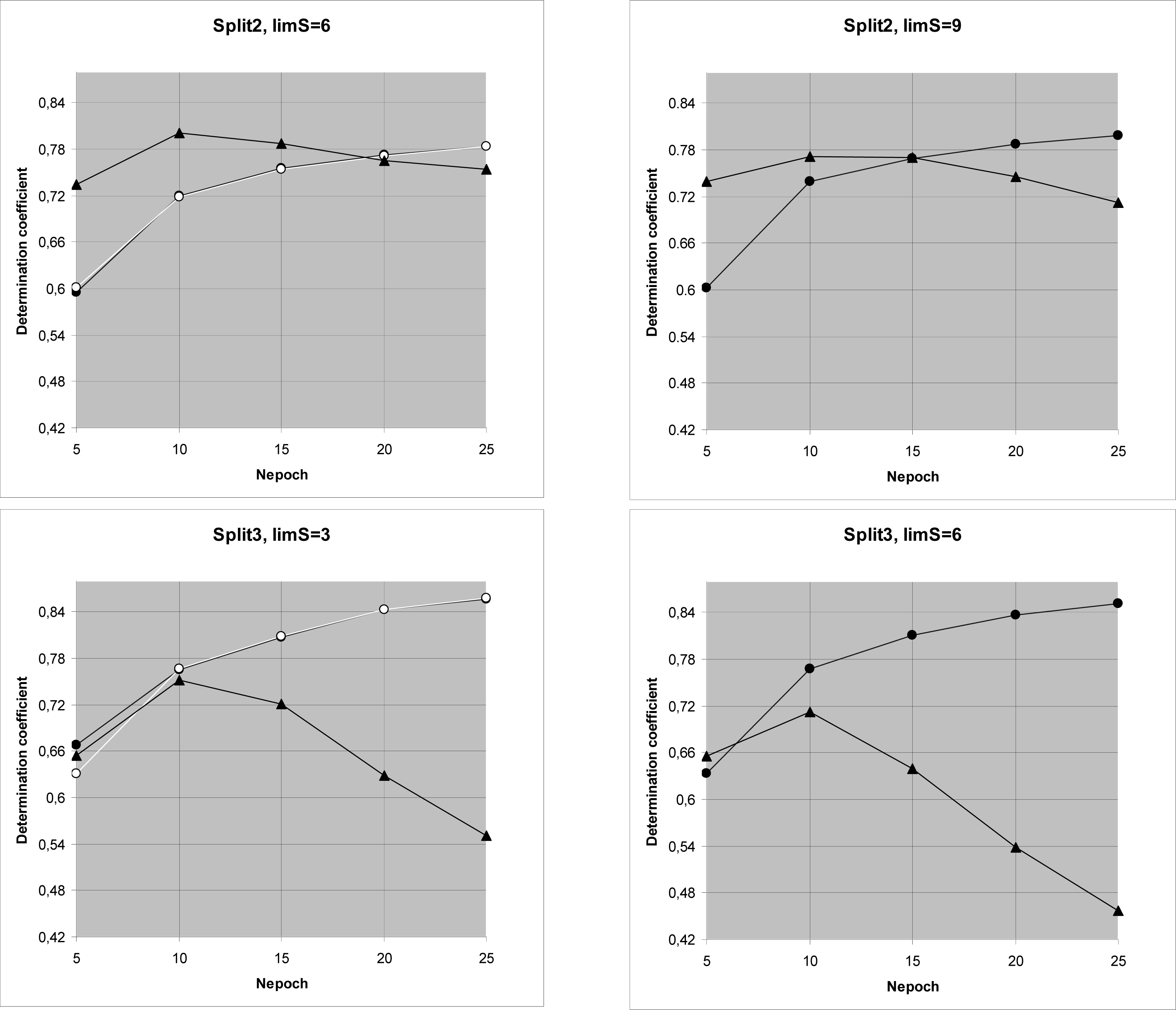
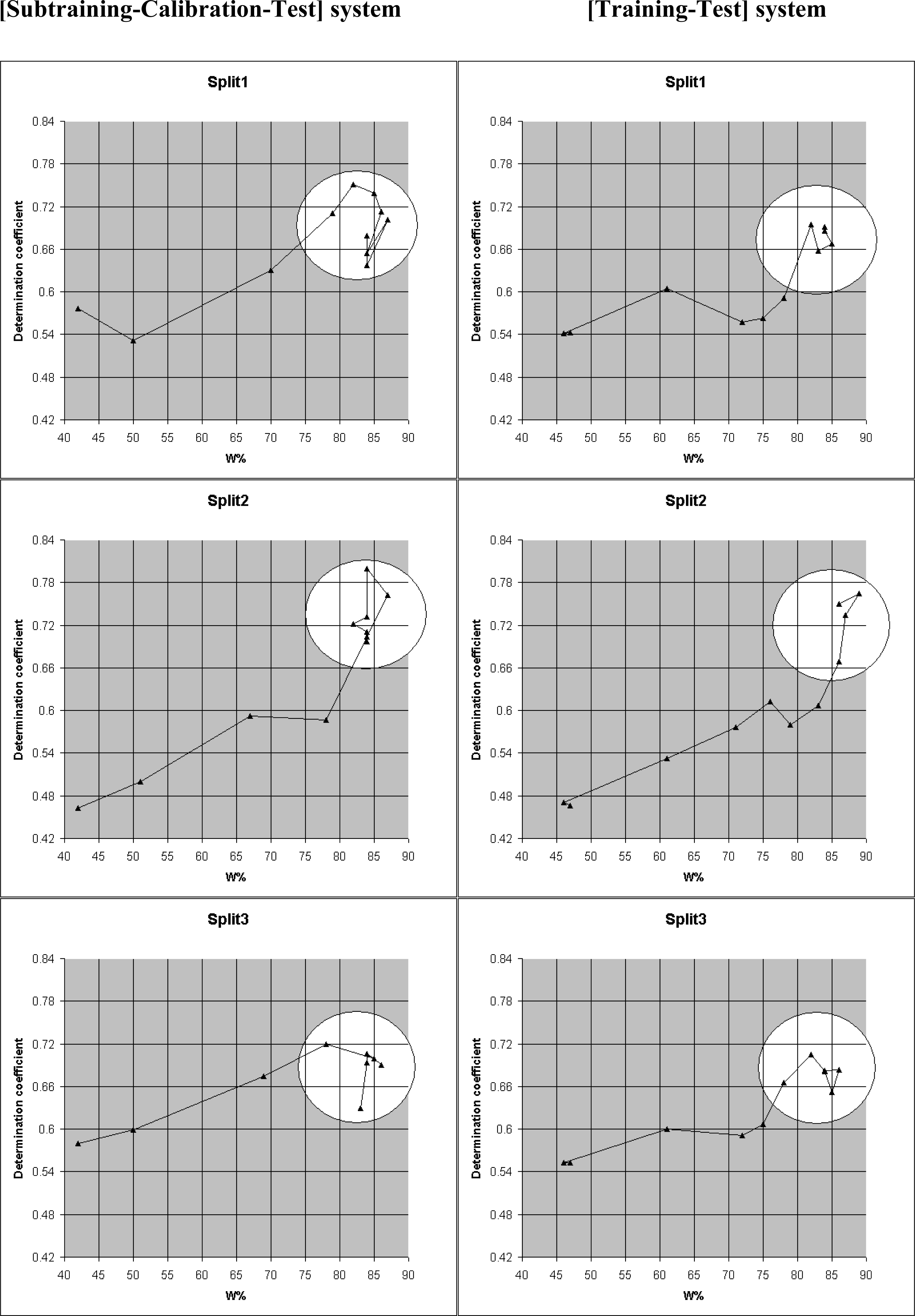
- - Optimal descriptors calculated by the Monte Carlo method can provide reasonable prediction for the carcinogenicity log(TD50).
- - Blocking of rare SMILES attributes can improve statistical quality of the predicting. Splits into subtraining, calibration and test sets, as well splits into the training and test sets have influence to statistical characteristics of the models. In our case, in three splits examined in this study these characteristics are similar.
- - The correlation balance, i.e., the [Subtraining-Calibration-Test] system gave models which are better in comparison with models obtained with the more traditional [Training-Test] system.
Supplementary Materials

| CAS No Split1 | CAS No Split2 | CAS No Split3 | |
|---|---|---|---|
| Subtraining set | |||
| 1. | 75-07-0 | 75-07-0 | 75-07-0 |
| 2. | 60-35-5 | 60-35-5 | 60-35-5 |
| 3. | 34627-78-6 | 53-96-3 | 53-96-3 |
| 4. | 4075-79-0 | 7008-42-6 | 7008-42-6 |
| 5. | 53-96-3 | 79-06-1 | 79-06-1 |
| 6. | 79-06-1 | 3688-53-7 | 107-13-1 |
| 7. | 107-13-1 | 81-49-2 | 3688-53-7 |
| 8. | 3688-53-7 | 3775-55-1 | 81-49-2 |
| 9. | 81-49-2 | 99-57-0 | 3775-55-1 |
| 10. | 3775-55-1 | 117-79-3 | 99-57-0 |
| 11. | 712-68-5 | 97-56-3 | 121-88-0 |
| 12. | 99-57-0 | 10589-74-9 | 117-79-3 |
| 13. | 121-88-0 | 140-57-8 | 2432-99-7 |
| 14. | 117-79-3 | 1912-24-9 | 10589-74-9 |
| 15. | 60142-96-3 | 115-02-6 | 115-02-6 |
| 16. | 2432-99-7 | 17967-53-9 | 17967-53-9 |
| 17. | 10589-74-9 | 50-32-8 | 71-43-2 |
| 18. | 17967-53-9 | 3296-90-0 | 92-87-5 |
| 19. | 30516-87-1 | 542-88-1 | 50-32-8 |
| 20. | 71-43-2 | 2475-45-8 | 14504-15-5 |
| 21. | 92-87-5 | 75-27-4 | 2475-45-8 |
| 22. | 50-32-8 | 51333-22-3 | 74-96-4 |
| 23. | 14504-15-5 | 3068-88-0 | 3068-88-0 |
| 24. | 3296-90-0 | 63-25-2 | 63-25-2 |
| 25. | 85-68-7 | 56-23-5 | 56-23-5 |
| 26. | 3068-88-0 | 120-80-9 | 60391-92-6 |
| 27. | 331-39-5 | 305-03-3 | 305-03-3 |
| 28. | 63-25-2 | 77439-76-0 | 37087-94-8 |
| 29. | 56-23-5 | 37087-94-8 | 5131-60-2 |
| 30. | 305-03-3 | 95-83-0 | 75-88-7 |
| 31. | 37087-94-8 | 150-68-5 | 50892-23-4 |
| 32. | 75-88-7 | 10473-70-8 | 108-90-7 |
| 33. | 50892-23-4 | 1897-45-6 | 107-30-2 |
| 34. | 65089-17-0 | 102-50-1 | 150-68-5 |
| 35. | 108-90-7 | 80-08-0 | 126-99-8 |
| 36. | 107-30-2 | 50-29-3 | 1897-45-6 |
| 37. | 150-68-5 | 53-43-0 | 102-50-1 |
| 38. | 126-99-8 | 853-23-6 | 120-71-8 |
| 39. | 1897-45-6 | 63019-65-8 | 80-08-0 |
| 40. | 102-50-1 | 16338-97-9 | 853-23-6 |
| 41. | 120-71-8 | 720-69-4 | 16338-97-9 |
| 42. | 1163-19-5 | 95-80-7 | 720-69-4 |
| 43. | 853-23-6 | 96-12-8 | 96-12-8 |
| 44. | 16338-97-9 | 10318-26-0 | 10318-26-0 |
| 45. | 720-69-4 | 106-93-4 | 106-93-4 |
| 46. | 4106-66-5 | 1717-00-6 | 106-46-7 |
| 47. | 96-12-8 | 107-06-2 | 107-06-2 |
| 48. | 10318-26-0 | 62-73-7 | 101-90-6 |
| 49. | 106-93-4 | 56-53-1 | 3276-41-3 |
| 50. | 7572-29-4 | 101-90-6 | 119-84-6 |
| 51. | 106-46-7 | 5803-51-0 | 5803-51-0 |
| 52. | 105-55-5 | 59-35-8 | 91-93-0 |
| 53. | 3276-41-3 | 55738-54-0 | 60-11-7 |
| 54. | 91-93-0 | 121-69-7 | 59-35-8 |
| 55. | 4164-28-7 | 26049-69-4 | 513-37-1 |
| 56. | 513-37-1 | 513-37-1 | 106-89-8 |
| 57. | 106-89-8 | 106-89-8 | 150-69-6 |
| 58. | 150-69-6 | 140-88-5 | 16301-26-1 |
| 59. | 16301-26-1 | 64-17-5 | 57497-29-7 |
| 60. | 75-21-8 | 16301-26-1 | 75-21-8 |
| 61. | 117-81-7 | 57497-29-7 | 86386-73-4 |
| 62. | 110559-84-7 | 75-21-8 | 69112-98-7 |
| 63. | 86386-73-4 | 96724-44-6 | 110-00-9 |
| 64. | 69112-98-7 | 86386-73-4 | 67730-11-4 |
| 65. | 93957-54-1 | 363-17-7 | 56-40-6 |
| 66. | 98-01-1 | 3570-75-0 | 87-68-3 |
| 67. | 56-40-6 | 110-00-9 | 319-84-6 |
| 68. | 319-84-6 | 98-01-1 | 67-72-1 |
| 69. | 67-72-1 | 67730-11-4 | 26049-70-7 |
| 70. | 18774-85-1 | 56-40-6 | 122-66-7 |
| 71. | 26049-70-7 | 87-68-3 | 53-95-2 |
| 72. | 122-66-7 | 67-72-1 | 129-43-1 |
| 73. | 53-95-2 | 680-31-9 | 96724-45-7 |
| 74. | 129-43-1 | 26049-70-7 | 13743-07-2 |
| 75. | 96724-45-7 | 53-95-2 | 71752-70-0 |
| 76. | 71752-70-0 | 84545-30-2 | 100643-96-7 |
| 77. | 100643-96-7 | 100643-96-7 | 76180-96-6 |
| 78. | 76180-96-6 | 76180-96-6 | 115-11-7 |
| 79. | 115-11-7 | 15503-86-3 | 542-56-3 |
| 80. | 542-56-3 | 115-11-7 | 54-85-3 |
| 81. | 303-34-4 | 542-56-3 | 303-34-4 |
| 82. | 76956-02-0 | 54-85-3 | 108-78-1 |
| 83. | 148-82-3 | 303-34-4 | 148-82-3 |
| 84. | 149-30-4 | 76956-02-0 | 149-30-4 |
| 85. | 5834-17-3 | 108-78-1 | 934-00-9 |
| 86. | 934-00-9 | 148-82-3 | 298-81-7 |
| 87. | 298-81-7 | 60-56-0 | 598-55-0 |
| 88. | 598-55-0 | 5834-17-3 | 55-80-1 |
| 89. | 21638-36-8 | 298-81-7 | 21638-36-8 |
| 90. | 63412-06-6 | 1634-04-4 | 63412-06-6 |
| 91. | 598-57-2 | 21340-68-1 | 14026-03-0 |
| 92. | 33868-17-6 | 21638-36-8 | 598-57-2 |
| 93. | 443-48-1 | 63412-06-6 | 76014-81-8 |
| 94. | 39801-14-4 | 14026-03-0 | 64091-91-4 |
| 95. | 50-07-7 | 76014-81-8 | 90-94-8 |
| 96. | 3771-19-5 | 64091-91-4 | 2385-85-5 |
| 97. | 2243-62-1 | 90-94-8 | 39801-14-4 |
| 98. | 139-94-6 | 39801-14-4 | 50-07-7 |
| 99. | 99-59-2 | 50-07-7 | 58139-48-3 |
| 100. | 2122-86-3 | 58139-48-3 | 2243-62-1 |
| 101. | 2578-75-8 | 389-08-2 | 139-94-6 |
| 102. | 53757-28-1 | 2243-62-1 | 99-59-2 |
| 103. | 24554-26-5 | 91-59-8 | 91-23-6 |
| 104. | 600-24-8 | 139-94-6 | 600-24-8 |
| 105. | 1836-75-5 | 99-59-2 | 1836-75-5 |
| 106. | 607-57-8 | 59-87-0 | 607-57-8 |
| 107. | 75-52-5 | 75198-31-1 | 555-84-0 |
| 108. | 38777-13-8 | 36133-88-7 | 38777-13-8 |
| 109. | 83335-32-4 | 4812-22-0 | 83335-32-4 |
| 110. | 89911-78-4 | 555-84-0 | 89911-79-5 |
| 111. | 96806-35-8 | 51-75-2 | 89911-78-4 |
| 112. | 56222-35-6 | 38777-13-8 | 96806-35-8 |
| 113. | 760-60-1 | 83335-32-4 | 760-60-1 |
| 114. | 937-25-7 | 89911-78-4 | 937-25-7 |
| 115. | 75881-22-0 | 96806-35-8 | 13256-11-6 |
| 116. | 38347-74-9 | 760-60-1 | 75881-22-0 |
| 117. | 64005-62-5 | 937-25-7 | 38347-74-9 |
| 118. | 1133-64-8 | 13256-11-6 | 91308-70-2 |
| 119. | 51542-33-7 | 38347-74-9 | 1133-64-8 |
| 120. | 60599-38-4 | 1133-64-8 | 60599-38-4 |
| 121. | 62-75-9 | 55-18-5 | 62-75-9 |
| 122. | 156-10-5 | 62-75-9 | 156-10-5 |
| 123. | 10595-95-6 | 156-10-5 | 20917-49-1 |
| 124. | 20917-49-1 | 42579-28-2 | 42579-28-2 |
| 125. | 42579-28-2 | 86451-37-8 | 86451-37-8 |
| 126. | 86451-37-8 | 70415-59-7 | 70415-59-7 |
| 127. | 26921-68-6 | 16219-98-0 | 55984-51-5 |
| 128. | 70415-59-7 | 59-89-2 | 16219-98-0 |
| 129. | 16219-98-0 | 5632-47-3 | 614-00-6 |
| 130. | 614-00-6 | 930-55-2 | 59-89-2 |
| 131. | 59-89-2 | 81795-07-5 | 5632-47-3 |
| 132. | 26541-51-5 | 3096-50-2 | 100-75-4 |
| 133. | 611-23-4 | 101-80-4 | 930-55-2 |
| 134. | 303-47-9 | 60102-37-6 | 26541-51-5 |
| 135. | 3096-50-2 | 62-44-2 | 611-23-4 |
| 136. | 60102-37-6 | 60-80-0 | 303-47-9 |
| 137. | 62-44-2 | 77-09-8 | 3096-50-2 |
| 138. | 77-09-8 | 7227-91-0 | 77-09-8 |
| 139. | 7227-91-0 | 842-07-9 | 7227-91-0 |
| 140. | 90-43-7 | 50-33-9 | 50-33-9 |
| 141. | 51-03-6 | 122-60-1 | 90-43-7 |
| 142. | 29069-24-7 | 51-03-6 | 51-03-6 |
| 143. | 50-24-8 | 1955-45-9 | 1955-45-9 |
| 144. | 671-16-9 | 29069-24-7 | 29069-24-7 |
| 145. | 1120-71-4 | 816-57-9 | 57-57-8 |
| 146. | 57-57-8 | 75-56-9 | 13010-07-6 |
| 147. | 13010-07-6 | 599-79-1 | 81-54-9 |
| 148. | 51-52-5 | 2318-18-5 | 2425-85-6 |
| 149. | 2425-85-6 | 10048-13-2 | 480-54-6 |
| 150. | 480-54-6 | 18883-66-4 | 2318-18-5 |
| 151. | 94-59-7 | 96-09-3 | 10048-13-2 |
| 152. | 2318-18-5 | 95-06-7 | 18883-66-4 |
| 153. | 10048-13-2 | 23031-25-6 | 95-06-7 |
| 154. | 18883-66-4 | 127-18-4 | 116-14-3 |
| 155. | 96-09-3 | 116-14-3 | 109-99-9 |
| 156. | 95-06-7 | 509-14-8 | 509-14-8 |
| 157. | 127-18-4 | 139-65-1 | 52-24-4 |
| 158. | 109-99-9 | 62-56-6 | 139-65-1 |
| 159. | 62-56-6 | 68-76-8 | 88-19-7 |
| 160. | 88-19-7 | 538-23-8 | 68-76-8 |
| 161. | 68-76-8 | 88-06-2 | 76-25-5 |
| 162. | 76-25-5 | 96-18-4 | 75-25-2 |
| 163. | 75-25-2 | 2489-77-2 | 137-17-7 |
| 164. | 51-79-6 | 51-79-6 | 51-79-6 |
| 165. | 88-12-0 | 593-60-2 | 88-12-0 |
| Calibration set | |||
| 1. | 18523-69-8 | 18523-69-8 | 18523-69-8 |
| 2. | 7008-42-6 | 34627-78-6 | 34627-78-6 |
| 3. | 2835-39-4 | 4075-79-0 | 4075-79-0 |
| 4. | 760-56-5 | 107-13-1 | 760-56-5 |
| 5. | 82-28-0 | 1162-65-8 | 82-28-0 |
| 6. | 119-34-6 | 760-56-5 | 712-68-5 |
| 7. | 121-66-4 | 82-28-0 | 119-34-6 |
| 8. | 97-56-3 | 712-68-5 | 121-66-4 |
| 9. | 61-82-5 | 119-34-6 | 97-56-3 |
| 10. | 115-02-6 | 60142-96-3 | 60142-96-3 |
| 11. | 103-33-3 | 61-82-5 | 61-82-5 |
| 12. | 88133-11-3 | 25843-45-2 | 1912-24-9 |
| 13. | 271-89-6 | 30516-87-1 | 103-33-3 |
| 14. | 542-88-1 | 88133-11-3 | 25843-45-2 |
| 15. | 2475-45-8 | 71-43-2 | 30516-87-1 |
| 16. | 75-27-4 | 92-87-5 | 88133-11-3 |
| 17. | 74-96-4 | 271-89-6 | 271-89-6 |
| 18. | 51333-22-3 | 14504-15-5 | 3296-90-0 |
| 19. | 106-99-0 | 2784-94-3 | 542-88-1 |
| 20. | 75-65-0 | 106-99-0 | 2784-94-3 |
| 21. | 60391-92-6 | 75-65-0 | 51333-22-3 |
| 22. | 115-28-6 | 115-28-6 | 106-99-0 |
| 23. | 101-79-1 | 101-79-1 | 75-65-0 |
| 24. | 77439-76-0 | 5131-60-2 | 85-68-7 |
| 25. | 5131-60-2 | 75-88-7 | 115-28-6 |
| 26. | 593-70-4 | 65089-17-0 | 101-79-1 |
| 27. | 54749-90-5 | 107-30-2 | 77439-76-0 |
| 28. | 52214-84-3 | 126-99-8 | 65089-17-0 |
| 29. | 637-07-0 | 52214-84-3 | 593-70-4 |
| 30. | 123-73-9 | 637-07-0 | 10473-70-8 |
| 31. | 50-18-0 | 120-71-8 | 52214-84-3 |
| 32. | 80-08-0 | 123-73-9 | 637-07-0 |
| 33. | 50-29-3 | 50-18-0 | 123-73-9 |
| 34. | 63019-65-8 | 1163-19-5 | 50-18-0 |
| 35. | 95-80-7 | 4106-66-5 | 50-29-3 |
| 36. | 56654-52-5 | 56654-52-5 | 1163-19-5 |
| 37. | 1717-00-6 | 7572-29-4 | 63019-65-8 |
| 38. | 91-94-1 | 106-46-7 | 95-80-7 |
| 39. | 107-06-2 | 91-94-1 | 56654-52-5 |
| 40. | 62-73-7 | 111-46-6 | 1717-00-6 |
| 41. | 685-91-6 | 3276-41-3 | 7572-29-4 |
| 42. | 111-46-6 | 119-84-6 | 91-94-1 |
| 43. | 56-53-1 | 94-58-6 | 62-73-7 |
| 44. | 119-84-6 | 91-93-0 | 685-91-6 |
| 45. | 94-58-6 | 65176-75-2 | 111-46-6 |
| 46. | 5803-51-0 | 60-11-7 | 56-53-1 |
| 47. | 65176-75-2 | 551-92-8 | 94-58-6 |
| 48. | 60-11-7 | 123-91-1 | 65176-75-2 |
| 49. | 59-35-8 | 57-63-6 | 551-92-8 |
| 50. | 551-92-8 | 150-69-6 | 26049-69-4 |
| 51. | 26049-69-4 | 100-41-4 | 123-91-1 |
| 52. | 123-91-1 | 96-45-7 | 13256-06-9 |
| 53. | 13256-06-9 | 117-81-7 | 57-63-6 |
| 54. | 57-63-6 | 110559-84-7 | 140-88-5 |
| 55. | 140-88-5 | 38434-77-4 | 64-17-5 |
| 56. | 64-17-5 | 69112-98-7 | 100-41-4 |
| 57. | 57497-29-7 | 93957-54-1 | 96-45-7 |
| 58. | 100-41-4 | 556-52-5 | 117-81-7 |
| 59. | 96-45-7 | 517-28-2 | 96724-44-6 |
| 60. | 96724-44-6 | 118-74-1 | 110559-84-7 |
| 61. | 38434-77-4 | 319-84-6 | 38434-77-4 |
| 62. | 363-17-7 | 122-66-7 | 363-17-7 |
| 63. | 110-00-9 | 306-83-2 | 93957-54-1 |
| 64. | 67730-11-4 | 129-43-1 | 3570-75-0 |
| 65. | 556-52-5 | 33389-36-5 | 556-52-5 |
| 66. | 517-28-2 | 71752-70-0 | 517-28-2 |
| 67. | 118-74-1 | 5208-87-7 | 118-74-1 |
| 68. | 87-68-3 | 21416-87-5 | 680-31-9 |
| 69. | 680-31-9 | 53-86-1 | 26049-68-3 |
| 70. | 26049-68-3 | 86315-52-8 | 306-83-2 |
| 71. | 306-83-2 | 78-59-1 | 33389-36-5 |
| 72. | 13743-07-2 | 3778-73-2 | 5208-87-7 |
| 73. | 33389-36-5 | 143-50-0 | 21416-87-5 |
| 74. | 5208-87-7 | 5989-27-5 | 84545-30-2 |
| 75. | 84545-30-2 | 77500-04-0 | 53-86-1 |
| 76. | 53-86-1 | 149-30-4 | 15503-86-3 |
| 77. | 15503-86-3 | 57-39-6 | 86315-52-8 |
| 78. | 86315-52-8 | 934-00-9 | 78-59-1 |
| 79. | 54-85-3 | 150-76-5 | 3778-73-2 |
| 80. | 78-59-1 | 598-55-0 | 143-50-0 |
| 81. | 3778-73-2 | 55-80-1 | 5989-27-5 |
| 82. | 143-50-0 | 70-25-7 | 76956-02-0 |
| 83. | 5989-27-5 | 129-15-7 | 57-39-6 |
| 84. | 108-78-1 | 63642-17-1 | 60-56-0 |
| 85. | 57-39-6 | 452-86-8 | 150-76-5 |
| 86. | 60-56-0 | 56-49-5 | 1634-04-4 |
| 87. | 150-76-5 | 101-14-4 | 70-25-7 |
| 88. | 1634-04-4 | 838-88-0 | 129-15-7 |
| 89. | 21340-68-1 | 598-57-2 | 63642-17-1 |
| 90. | 70-25-7 | 33868-17-6 | 98-85-1 |
| 91. | 63642-17-1 | 443-48-1 | 452-86-8 |
| 92. | 98-85-1 | 3771-19-5 | 56-49-5 |
| 93. | 452-86-8 | 139-13-9 | 101-14-4 |
| 94. | 56-49-5 | 2578-75-8 | 838-88-0 |
| 95. | 101-14-4 | 531-82-8 | 33868-17-6 |
| 96. | 838-88-0 | 24554-26-5 | 443-48-1 |
| 97. | 101-61-1 | 91-23-6 | 315-22-0 |
| 98. | 76014-81-8 | 98-95-3 | 3771-19-5 |
| 99. | 64091-91-4 | 600-24-8 | 389-08-2 |
| 100. | 2385-85-5 | 1836-75-5 | 59-87-0 |
| 101. | 315-22-0 | 607-57-8 | 75198-31-1 |
| 102. | 58139-48-3 | 67-20-9 | 2122-86-3 |
| 103. | 389-08-2 | 75-52-5 | 36133-88-7 |
| 104. | 91-59-8 | 551-88-2 | 2578-75-8 |
| 105. | 139-13-9 | 5522-43-0 | 24554-26-5 |
| 106. | 59-87-0 | 607-35-2 | 4812-22-0 |
| 107. | 75198-31-1 | 16813-36-8 | 602-87-9 |
| 108. | 36133-88-7 | 89911-79-5 | 98-95-3 |
| 109. | 4812-22-0 | 92177-50-9 | 67-20-9 |
| 110. | 602-87-9 | 56222-35-6 | 51-75-2 |
| 111. | 91-23-6 | 55090-44-3 | 75-52-5 |
| 112. | 98-95-3 | 75881-20-8 | 551-88-2 |
| 113. | 67-20-9 | 75881-22-0 | 5522-43-0 |
| 114. | 555-84-0 | 684-93-5 | 607-35-2 |
| 115. | 51-75-2 | 55556-92-8 | 16813-36-8 |
| 116. | 551-88-2 | 82018-90-4 | 92177-50-9 |
| 117. | 607-35-2 | 75881-18-4 | 75896-33-2 |
| 118. | 16813-36-8 | 91308-70-2 | 56222-35-6 |
| 119. | 89911-79-5 | 91308-69-9 | 55090-44-3 |
| 120. | 92177-50-9 | 51542-33-7 | 75881-20-8 |
| 121. | 96806-34-7 | 60599-38-4 | 684-93-5 |
| 122. | 55090-44-3 | 924-16-3 | 55556-92-8 |
| 123. | 13256-11-6 | 1116-54-7 | 82018-90-4 |
| 124. | 684-93-5 | 621-64-7 | 75881-18-4 |
| 125. | 92177-49-6 | 10595-95-6 | 91308-69-9 |
| 126. | 55556-92-8 | 614-95-9 | 64005-62-5 |
| 127. | 82018-90-4 | 20917-49-1 | 51542-33-7 |
| 128. | 75881-18-4 | 26921-68-6 | 1116-54-7 |
| 129. | 91308-70-2 | 55984-51-5 | 55-18-5 |
| 130. | 91308-69-9 | 614-00-6 | 621-64-7 |
| 131. | 1116-54-7 | 68107-26-6 | 10595-95-6 |
| 132. | 55-18-5 | 78246-24-9 | 26921-68-6 |
| 133. | 621-64-7 | 303-47-9 | 78246-24-9 |
| 134. | 55984-51-5 | 14698-29-4 | 14698-29-4 |
| 135. | 68107-26-6 | 13752-51-7 | 101-80-4 |
| 136. | 78246-24-9 | 1825-21-4 | 13752-51-7 |
| 137. | 5632-47-3 | 50-24-8 | 60102-37-6 |
| 138. | 14698-29-4 | 671-16-9 | 62-44-2 |
| 139. | 101-80-4 | 1120-71-4 | 842-07-9 |
| 140. | 13752-51-7 | 57-57-8 | 122-60-1 |
| 141. | 1825-21-4 | 13010-07-6 | 50-24-8 |
| 142. | 842-07-9 | 51-52-5 | 671-16-9 |
| 143. | 50-33-9 | 81-54-9 | 1120-71-4 |
| 144. | 122-60-1 | 2425-85-6 | 816-57-9 |
| 145. | 1955-45-9 | 127-47-9 | 51-52-5 |
| 146. | 816-57-9 | 480-54-6 | 127-47-9 |
| 147. | 81-54-9 | 18559-94-9 | 18559-94-9 |
| 148. | 127-47-9 | 533-31-3 | 533-31-3 |
| 149. | 18559-94-9 | 77-46-3 | 96-09-3 |
| 150. | 599-79-1 | 811-97-2 | 77-46-3 |
| 151. | 533-31-3 | 40548-68-3 | 127-18-4 |
| 152. | 77-46-3 | 109-99-9 | 811-97-2 |
| 153. | 23031-25-6 | 52-24-4 | 40548-68-3 |
| 154. | 116-14-3 | 62-55-5 | 62-55-5 |
| 155. | 40548-68-3 | 789-61-7 | 789-61-7 |
| 156. | 509-14-8 | 141-90-2 | 141-90-2 |
| 157. | 52-24-4 | 88-19-7 | 62-56-6 |
| 158. | 62-55-5 | 76-25-5 | 88-06-2 |
| 159. | 789-61-7 | 75-25-2 | 42011-48-3 |
| 160. | 141-90-2 | 137-17-7 | 95-63-6 |
| 161. | 137-17-7 | 95-63-6 | 2489-77-2 |
| 162. | 95-63-6 | 55-63-0 | 55-63-0 |
| 163. | 55-63-0 | 126-72-7 | 126-72-7 |
| 164. | 126-72-7 | 66-22-8 | 66-22-8 |
| 165. | 108-05-4 | 108-05-4 | 108-05-4 |
| 166. | 75-02-5 | 75-02-5 | 75-02-5 |
| 167. | 2832-40-8 | 2832-40-8 | 2832-40-8 |
| Test set | |||
| 1. | 29611-03-8 | 29611-03-8 | 29611-03-8 |
| 2. | 1162-65-8 | 57-06-7 | 1162-65-8 |
| 3. | 57-06-7 | 2835-39-4 | 57-06-7 |
| 4. | 38514-71-5 | 38514-71-5 | 2835-39-4 |
| 5. | 140-57-8 | 121-88-0 | 38514-71-5 |
| 6. | 1912-24-9 | 121-66-4 | 140-57-8 |
| 7. | 25843-45-2 | 2432-99-7 | 33372-39-3 |
| 8. | 33372-39-3 | 103-33-3 | 75-27-4 |
| 9. | 2784-94-3 | 33372-39-3 | 869-01-2 |
| 10. | 869-01-2 | 74-96-4 | 331-39-5 |
| 11. | 120-80-9 | 85-68-7 | 120-80-9 |
| 12. | 95-83-0 | 869-01-2 | 95-83-0 |
| 13. | 10473-70-8 | 331-39-5 | 54749-90-5 |
| 14. | 117-10-2 | 60391-92-6 | 117-10-2 |
| 15. | 1192-28-5 | 50892-23-4 | 1192-28-5 |
| 16. | 53-43-0 | 108-90-7 | 53-43-0 |
| 17. | 79-43-6 | 593-70-4 | 4106-66-5 |
| 18. | 101-90-6 | 54749-90-5 | 79-43-6 |
| 19. | 55738-54-0 | 117-10-2 | 105-55-5 |
| 20. | 121-69-7 | 1192-28-5 | 55738-54-0 |
| 21. | 106-88-7 | 79-43-6 | 121-69-7 |
| 22. | 13073-35-3 | 685-91-6 | 4164-28-7 |
| 23. | 398-32-3 | 105-55-5 | 106-88-7 |
| 24. | 32852-21-4 | 4164-28-7 | 13073-35-3 |
| 25. | 3570-75-0 | 13256-06-9 | 398-32-3 |
| 26. | 67730-10-3 | 106-88-7 | 32852-21-4 |
| 27. | 26049-71-8 | 13073-35-3 | 98-01-1 |
| 28. | 21416-87-5 | 398-32-3 | 67730-10-3 |
| 29. | 77500-04-0 | 32852-21-4 | 18774-85-1 |
| 30. | 55-80-1 | 67730-10-3 | 26049-71-8 |
| 31. | 129-15-7 | 18774-85-1 | 77500-04-0 |
| 32. | 14026-03-0 | 26049-71-8 | 5834-17-3 |
| 33. | 90-94-8 | 26049-68-3 | 21340-68-1 |
| 34. | 531-82-8 | 96724-45-7 | 101-61-1 |
| 35. | 51325-35-0 | 13743-07-2 | 91-59-8 |
| 36. | 62-23-7 | 98-85-1 | 139-13-9 |
| 37. | 5522-43-0 | 101-61-1 | 53757-28-1 |
| 38. | 75896-33-2 | 2385-85-5 | 531-82-8 |
| 39. | 75881-20-8 | 315-22-0 | 51325-35-0 |
| 40. | 88208-16-6 | 2122-86-3 | 62-23-7 |
| 41. | 91308-71-3 | 53757-28-1 | 96806-34-7 |
| 42. | 53609-64-6 | 51325-35-0 | 92177-49-6 |
| 43. | 924-16-3 | 602-87-9 | 88208-16-6 |
| 44. | 40580-89-0 | 62-23-7 | 91308-71-3 |
| 45. | 614-95-9 | 96806-34-7 | 53609-64-6 |
| 46. | 100-75-4 | 75896-33-2 | 924-16-3 |
| 47. | 930-55-2 | 92177-49-6 | 40580-89-0 |
| 48. | 81795-07-5 | 88208-16-6 | 614-95-9 |
| 49. | 60-80-0 | 91308-71-3 | 68107-26-6 |
| 50. | 75-56-9 | 64005-62-5 | 81795-07-5 |
| 51. | 22571-95-5 | 53609-64-6 | 1825-21-4 |
| 52. | 811-97-2 | 40580-89-0 | 60-80-0 |
| 53. | 139-65-1 | 100-75-4 | 75-56-9 |
| 54. | 538-23-8 | 26541-51-5 | 94-59-7 |
| 55. | 88-06-2 | 611-23-4 | 599-79-1 |
| 56. | 96-18-4 | 90-43-7 | 22571-95-5 |
| 57. | 42011-48-3 | 94-59-7 | 23031-25-6 |
| 58. | 2489-77-2 | 22571-95-5 | 538-23-8 |
| 59. | 66-22-8 | 42011-48-3 | 96-18-4 |
| 60. | 593-60-2 | 75-01-4 | 593-60-2 |
| 61. | 75-01-4 | 88-12-0 | 75-01-4 |
| CAS No | SMILES | DCW(4) | Expr | Calc |
|---|---|---|---|---|
| Subtraining set | ||||
| 75-07-0 | CC=O | −1.6442255 | −0.541 | −0.782 |
| 60-35-5 | CC(N)=O | 2.4339941 | −0.484 | −0.326 |
| 34627-78-6 | CC(=O)OC(C=C)c1ccc2OCOc2c1 | 8.9723429 | 0.945 | 0.405 |
| 4075-79-0 | O=C(C)Nc1ccc(cc1)c2ccccc2 | 16.8254890 | 2.253 | 1.283 |
| 53-96-3 | CC(=O)NC1C=CC2=C3C=CC=CC3=CC2=C1 | 23.7041967 | 2.263 | 2.052 |
| 79-06-1 | C=CC(N)=O | 6.1553307 | 1.278 | 0.090 |
| 107-13-1 | C=CC#N | 0.4363647 | 0.497 | −0.549 |
| 3688-53-7 | O=[N+]([O−])c2ccc(/C=C(\c1ccco1)C(N)=O)o2 | 19.7219116 | 0.926 | 1.607 |
| 81-49-2 | O=C2c1ccccc1C(=O)c3c2c(N)c(Br)cc3Br | 10.6082785 | 0.918 | 0.588 |
| 3775-55-1 | Nc1nnc(o1)c2oc(cc2)[N+]([O−])=O | 19.5286009 | 1.728 | 1.585 |
| 712-68-5 | Nc1nnc(s1)c2oc(cc2)[N+]([O−])=O | 21.4765044 | 2.506 | 1.803 |
| 99-57-0 | Nc1cc(ccc1O)[N+]([O−])=O | 8.7582849 | −0.736 | 0.381 |
| 121-88-0 | Nc1ccc(cc1O)[N+]([O−])=O | 8.7582849 | 0.143 | 0.381 |
| 117-79-3 | Nc2ccc3C(=O)c1ccccc1C(=O)c3c2 | 10.4267880 | 0.344 | 0.568 |
| 60142-96-3 | NCC1(CC(=O)O)CCCCC1 | −3.0738151 | −1.533 | −0.942 |
| 2432-99-7 | O=C(O)CCCCCCCCCCN | −2.3822437 | −0.737 | −0.864 |
| 10589-74-9 | CCCCCN(N=O)C(N)=O | 28.9999825 | 2.462 | 2.644 |
| 17967-53-9 | CC(C)[N+](\[O−])=N/C(C)C | 41.1617896 | 4.686 | 4.004 |
| 30516-87-1 | CC1=CN(C(=O)NC1=O)C2CC(/N=[N+]=[N−])C(CO)O2 | −2.1058355 | −1.637 | −0.834 |
| 71-43-2 | c1ccccc1 | 3.2902364 | −0.335 | −0.230 |
| 92-87-5 | Nc1ccc(cc1)c2ccc(N)cc2 | 15.6117993 | 2.027 | 1.147 |
| 50-32-8 | c1cc2c3ccc4cccc5ccc(cc2cc1)c3c45 | 28.9921674 | 2.421 | 2.643 |
| 14504-15-5 | NC(=O)Cc2c([O−])on[n+]2Cc1ccccc1 | 4.7178230 | −0.260 | −0.071 |
| 3296-90-0 | OCC(CBr)(CBr)CO | 10.1582969 | 0.373 | 0.538 |
| 85-68-7 | O=C(OCc1ccccc1)c2ccccc2C(=O)OCCCC | 9.6647886 | −0.522 | 0.482 |
| 3068-88-0 | O=C1CC(C)O1 | 7.0229065 | 0.795 | 0.187 |
| 331-39-5 | Oc1ccc(/C=C/C(=O)O)cc1O | 2.7387186 | −0.217 | −0.292 |
| 63-25-2 | CNC(=O)Oc2cccc1ccccc12 | 12.8497971 | 1.154 | 0.839 |
| 56-23-5 | ClC(Cl)(Cl)Cl | 12.2869593 | 1.827 | 0.776 |
| 305-03-3 | O=C(O)CCCc1ccc(cc1)N(CCCl)CCCl | 26.8564822 | 2.531 | 2.404 |
| 37087-94-8 | CC1CC(C)CN(C1)S(=O)(=O)c2cc(C(=O)O)c(Cl)cc2 | 22.7615129 | 1.835 | 1.947 |
| 75-88-7 | ClCC(F)(F)F | 11.1755831 | 0.133 | 0.651 |
| 50892-23-4 | Cc2cccc(Nc1cc(Cl)nc(SCC(=O)O)n1)c2C | 19.0894905 | 1.871 | 1.536 |
| 65089-17-0 | Cc2cccc(Nc1cc(Cl)nc(SCC(=O)NCCO)n1)c2C | 17.8867308 | 1.752 | 1.402 |
| 108-90-7 | Clc1ccccc1 | 0.8393418 | −0.341 | −0.504 |
| 107-30-2 | COCCl | 21.7058832 | 1.166 | 1.829 |
| 150-68-5 | Clc1ccc(NC(=O)N(C)C)cc1 | 7.6668178 | 0.181 | 0.259 |
| 126-99-8 | C=C(Cl)C=C | 0.3865032 | −0.150 | −0.555 |
| 1897-45-6 | Clc1c(C#N)c(Cl)c(C#N)c(Cl)c1Cl | −1.4730550 | −0.931 | −0.763 |
| 102-50-1 | Nc1ccc(OC)cc1C | 3.4796799 | −0.535 | −0.209 |
| 120-71-8 | Nc1cc(C)ccc1OC | 6.7795818 | 0.146 | 0.160 |
| 1163-19-5 | Brc2c(Oc1c(Br)c(Br)c(Br)c(Br)c1Br)c(Br)c(Br)c(Br)c2 Br | 0.8059877 | −0.542 | −0.508 |
| 853-23-6 | CC(=O)OC2CCC3(C)C4CCC1(C)C(CCC1=O)C4CC=C 3C2 | 23.1543517 | 1.022 | 1.991 |
| 16338-97-9 | C=CCN(CC=C)N=O | 26.5787909 | 0.571 | 2.373 |
| 720-69-4 | O=[N+]([O−])c1ccc(o1)c2nc(N)nc(N)n2 | 15.5122743 | 2.114 | 1.136 |
| 4106-66-5 | Nc1ccc2c3ccccc3oc2c1 | 18.8006239 | 1.869 | 1.504 |
| 96-12-8 | BrC(CBr)CCl | 24.2664740 | 2.960 | 2.115 |
| 10318-26-0 | OC(C(O)CBr)C(O)C(O)CBr | 21.0738102 | 1.566 | 1.758 |
| 106-93-4 | BrCCBr | 13.4511485 | 2.092 | 0.906 |
| 7572-29-4 | ClC#CCl | 24.1260754 | 1.423 | 2.099 |
| 106-46-7 | Clc1ccc(Cl)cc1 | 4.3705653 | −0.642 | −0.109 |
| 105-55-5 | CCNC(=S)NCC | 12.9520877 | 0.741 | 0.850 |
| 3276-41-3 | O=NN1CC=CCO1 | 17.2055032 | 0.100 | 1.325 |
| 91-93-0 | COc1cc(ccc1/N=C=O)c2ccc(\N=C=O)c(OC)c2 | 1.4504491 | −0.740 | −0.436 |
| 4164-28-7 | CN(C)[N+]([O−])=O | 20.1348499 | 2.217 | 1.653 |
| 513-37-1 | C/C(C)=C\Cl | 19.4680508 | 0.455 | 1.578 |
| 106-89-8 | ClCC1CO1 | 15.6927349 | 1.495 | 1.156 |
| 150-69-6 | CCOc1ccc(cc1)NC(N)=O | 4.9437759 | −0.474 | −0.045 |
| 16301-26-1 | [O−]\[N+](CC)=N\CC | 29.8573580 | 3.667 | 2.740 |
| 75-21-8 | C1CO1 | 4.1677964 | 0.316 | −0.132 |
| 117-81-7 | CCC(CCCC)COC(=O)c1ccccc1C(=O)OCC(CC)CCCC | −2.5987356 | −0.263 | −0.889 |
| 110559-84-7 | O=C(NCC(C)=O)N(CC)N=O | 25.1884351 | 2.981 | 2.218 |
| 86386-73-4 | OC(Cn1cncn1)(Cn2cncn2)c3ccc(F)cc3F | 6.0321942 | 0.579 | 0.076 |
| 69112-98-7 | NC(=O)N(CCF)N=O | 24.3033326 | 3.034 | 2.119 |
| 93957-54-1 | O=C(O)CC(O)CC(O)/C=C/c2c(c1ccccc1n2C(C)C)c3ccc (F)cc3 | 14.6992645 | 0.517 | 1.045 |
| 98-01-1 | O=Cc1ccco1 | 6.3091859 | −0.852 | 0.107 |
| 56-40-6 | NCC(=O)O | −1.3873663 | −2.534 | −0.753 |
| 319-84-6 | ClC1C(Cl)C(Cl)C(Cl)C(Cl)C1Cl | 18.2269649 | 1.414 | 1.440 |
| 67-72-1 | ClC(Cl)(Cl)C(Cl)(Cl)Cl | 14.7243688 | 0.631 | 1.048 |
| 18774-85-1 | CCCCCCN(N=O)C(N)=O | 28.1722194 | 2.529 | 2.552 |
| 26049-70-7 | NNc1nc(cs1)c2ccc(cc2)[N+]([O−])=O | 20.6520759 | 1.867 | 1.711 |
| 122-66-7 | N(Nc1ccccc1)c2ccccc2 | 18.1209496 | 1.518 | 1.428 |
| 53-95-2 | CC(=O)N(O)C1C=CC2=C3C=CC=CC3=CC2=C1 | 23.9896850 | 2.384 | 2.084 |
| 129-43-1 | O=C3c1ccccc1C(=O)c2c3cccc2O | 2.8757163 | 0.380 | −0.277 |
| 96724-45-7 | O=C(NCC)N(N=O)CCO | 21.7630490 | 2.458 | 1.835 |
| 71752-70-0 | O=C(N)N(N=O)CCCO | 17.2624478 | 2.177 | 1.332 |
| 100643-96-7 | O=C2Nc1ccc(cc1C2(C)C)C=3CCC(=O)NN=3 | 22.0312469 | 2.107 | 1.865 |
| 76180-96-6 | Nc3nc2c(ccc1ncccc12)n3C | 21.3468133 | 2.388 | 1.788 |
| 115-11-7 | C=C(C)C | 0.3184457 | −1.801 | −0.562 |
| 542-56-3 | CC(C)CON=O | 8.3162583 | 0.280 | 0.332 |
| 303-34-4 | CC(C)(O)C(O)(C(C)OC)C(=O)OCC1=CCN2CCC(OC(=O)C(\C)=C\C)C12 | 31.4970206 | 3.024 | 2.923 |
| 76956-02-0 | OCc3nc(NCCCOc2cc(CN1CCCCC1)ccc2)n(C)n3 | 12.5193481 | −0.125 | 0.802 |
| 148-82-3 | O=C(O)C(N)Cc1ccc(cc1)N(CCCl)CCCl | 41.9895654 | 3.512 | 4.096 |
| 149-30-4 | S=C1Nc2ccccc2S1 | 4.9343382 | −0.313 | −0.046 |
| 5834-17-3 | COc1cc2c3ccccc3oc2cc1N | 15.3424654 | 0.866 | 1.117 |
| 934-00-9 | COc1cccc(O)c1O | −1.6426353 | 0.459 | −0.782 |
| 298-81-7 | COc1c3occc3cc2C=CC(=O)Oc12 | 12.9007718 | 0.824 | 0.844 |
| 598-55-0 | NC(=O)OC | 2.7475976 | 0.123 | −0.291 |
| 21638-36-8 | O=[N+]([O−])c2ccc(/C=N/N1CC(C)NC1=O)o2 | 15.3657507 | 1.649 | 1.120 |
| 63412-06-6 | O=C(N(C)N=O)c1ccccc1 | 25.3611674 | 1.706 | 2.237 |
| 598-57-2 | [O−][N+](=O)CN | 9.4966339 | 0.641 | 0.464 |
| 33868-17-6 | N#CN(C)N=O | 24.8721377 | 2.249 | 2.183 |
| 443-48-1 | Cc1ncc([N+]([O−])=O)n1CCO | 2.0019404 | −0.501 | −0.374 |
| 39801-14-4 | ClC13C5(Cl)C2(Cl)C4C(Cl)(C(Cl)(Cl)C12Cl)C3(Cl)C4 (Cl)C5(Cl)Cl | 23.6405290 | 2.544 | 2.045 |
| 50-07-7 | NC(=O)OCC3C=1C(=O)C(N)=C(C)C(=O)C=1N4CC2 NC2C34OC | 46.6793245 | 5.509 | 4.621 |
| 3771-19-5 | O=C(O)C(C)(C)Oc1ccc(cc1)C3CCCc2ccccc23 | 15.0473711 | 1.451 | 1.084 |
| 2243-62-1 | Nc2cccc1c2cccc1N | 6.3106925 | 0.357 | 0.107 |
| 139-94-6 | O=C(Nc1ncc(s1)[N+]([O−])=O)NCC | 6.7942596 | 0.218 | 0.161 |
| 99-59-2 | Nc1cc(ccc1OC)[N+]([O−])=O | 15.7194316 | 0.494 | 1.159 |
| 2122-86-3 | O=C1NN=C(O1)c2oc(cc2)[N+]([O−])=O | 17.1616511 | 1.360 | 1.321 |
| 2578-75-8 | O=C(C)Nc1nnc(s1)c2ccc(o2)[N+]([O−])=O | 19.6066702 | 1.459 | 1.594 |
| 53757-28-1 | [O−][N+](=O)c1ccc(o1)c2cscn2 | 17.5109445 | 1.407 | 1.360 |
| 24554-26-5 | O=CNc1nc(cs1)c2ccc(o2)[N+]([O−])=O | 18.1182161 | 1.750 | 1.428 |
| 600-24-8 | CC(CC)[N+]([O−])=O | 10.7916363 | −0.443 | 0.608 |
| 1836-75-5 | Clc2cc(Cl)ccc2Oc1ccc(cc1)[N+]([O−])=O | 5.0065304 | −0.170 | −0.038 |
| 607-57-8 | [O−][N+](=O)C1C=CC2=C3C=CC=CC3=CC2=C1 | 33.1141590 | 2.870 | 3.104 |
| 75-52-5 | [O−][N+](C)=O | 19.9552121 | 0.179 | 1.633 |
| 38777-13-8 | CC(C)Oc1ccccc1OC(=O)N(C)N=O | 30.1163221 | 2.816 | 2.769 |
| 83335-32-4 | FC(F)(F)CCCN(CCCC(F)(F)F)N=O | 20.6003220 | 2.551 | 1.705 |
| 89911-78-4 | O=NN(CCO)CC(O)CO | 23.8214739 | 1.439 | 2.065 |
| 96806-35-8 | O=C(NCCCl)N(N=O)CC(C)O | 30.0147037 | 2.380 | 2.758 |
| 56222-35-6 | CC(O)CN(CCO)N=O | 22.4227138 | 1.181 | 1.909 |
| 760-60-1 | CC(C)CN(N=O)C(=O)N | 24.4205969 | 1.487 | 2.132 |
| 937-25-7 | O=NN(C)c1ccc(F)cc1 | 31.5388819 | 2.781 | 2.928 |
| 75881-22-0 | CN(CCCCCCCCCC)N=O | 21.5702225 | 2.201 | 1.813 |
| 38347-74-9 | O=C1OCCN1N=O | 16.7506150 | 2.479 | 1.275 |
| 64005-62-5 | O=NN(CCCCC)C(=O)OCC | 29.8114261 | 2.270 | 2.735 |
| 1133-64-8 | O=NN2CCCCC2c1cccnc1 | 25.2879439 | 1.206 | 2.229 |
| 51542-33-7 | CN(N=O)C(=O)Nc1nc2ccccc2s1 | 28.6323803 | 2.320 | 2.603 |
| 60599-38-4 | O=C(C)CN(CC(=O)C)N=O | 28.7233886 | 2.508 | 2.613 |
| 62-75-9 | CN(C)N=O | 28.9349431 | 2.888 | 2.637 |
| 156-10-5 | O=Nc2ccc(Nc1ccccc1)cc2 | 18.9993753 | −0.006 | 1.526 |
| 10595-95-6 | CCN(C)N=O | 32.7168392 | 3.244 | 3.060 |
| 20917-49-1 | O=NN1CCCCCCC1 | 23.6797366 | 3.575 | 2.049 |
| 42579-28-2 | O=C1NC(=O)CN1N=O | 19.2961524 | 0.469 | 1.559 |
| 86451-37-8 | CN(N=O)CC(O)CO | 21.1388672 | 2.317 | 1.765 |
| 26921-68-6 | CN(N=O)CCO | 25.9729565 | 1.907 | 2.306 |
| 70415-59-7 | CN(N=O)CCCO | 20.2587809 | 1.852 | 1.667 |
| 16219-98-0 | O=NN(C)c1ccccn1 | 24.9818346 | 2.807 | 2.195 |
| 614-00-6 | O=NN(C)c1ccccc1 | 26.3316239 | 2.982 | 2.346 |
| 59-89-2 | O=NN1CCOCC1 | 21.4019649 | 3.028 | 1.795 |
| 26541-51-5 | O=NN1CCSCC1 | 24.3742548 | 1.390 | 2.127 |
| 611-23-4 | Cc1ccccc1N=O | 10.7414983 | 0.378 | 0.603 |
| 303-47-9 | O=C(O)C(Cc1ccccc1)NC(=O)c2cc(Cl)c3CC(C)OC(=O) c3c2O | 27.3969214 | 3.593 | 2.465 |
| 3096-50-2 | CC(=O)Nc2ccc3c1ccccc1C(=O)c3c2 | 9.8204373 | 1.585 | 0.500 |
| 60102-37-6 | CN1CCC2OC(=O)C3(CC(C)C(C)(O)C(=O)OCC(=CC1)C2=O)OC3C | 22.8541422 | 2.617 | 1.957 |
| 62-44-2 | CCOc1ccc(cc1)NC(C)=O | 6.9861875 | −0.843 | 0.183 |
| 77-09-8 | Oc1ccc(cc1)C3(OC(=O)c2ccccc23)c4ccc(O)cc4 | 6.3745131 | −0.452 | 0.115 |
| 7227-91-0 | CN(C)/N=N/c1ccccc1 | 15.5075709 | 1.810 | 1.136 |
| 90-43-7 | Oc2ccccc2c1ccccc1 | 4.7845818 | −0.134 | −0.063 |
| 51-03-6 | CCCc1cc2OCOc2cc1COCCOCCOCCCC | 8.6169629 | −0.272 | 0.365 |
| 29069-24-7 | ClCCN(CCCl)c1ccc(cc1)CCCC(=O)OCC(=O)C5(O)CC C4C3CCC2=CC(=O)C=CC2(C)C3C(O)CC45C | 26.4791878 | 1.527 | 2.362 |
| 50-24-8 | OCC(=O)C4(O)CCC3C2CCC1=CC(=O)C=CC1(C)C2C (O)CC34C | 24.1947047 | 2.372 | 2.107 |
| 671-16-9 | CC(C)NC(=O)c1ccc(CNNC)cc1 | 15.0574555 | 1.742 | 1.085 |
| 1120-71-4 | O=S1(=O)CCCO1 | 6.0564342 | 1.503 | 0.079 |
| 57-57-8 | O=C1CCO1 | 10.5571479 | 1.693 | 0.582 |
| 13010-07-6 | N/C(=N/[N+]([O−])=O)N(CCC)N=O | 36.6885548 | 2.126 | 3.504 |
| 51-52-5 | S=C1NC(CCC)=CC(=O)N1 | 10.2034731 | 1.094 | 0.543 |
| 2425-85-6 | [O−][N+](=O)c3cc(C)ccc3N\N=C1\c2ccccc2C=CC1=O | −6.2022200 | −0.581 | −1.292 |
| 480-54-6 | O=C1OCC3=CCN2CCC(OC(=O)C(/CC(C)C1(O)CO)=C\C)C23 | 4.9508078 | −0.390 | −0.045 |
| 94-59-7 | C=CCc1ccc2OCOc2c1 | 5.7835004 | −0.434 | 0.048 |
| 2318-18-5 | O=C1OC2CCN(C)CC=C(COC(=O)C(C)(O)C(C)C\C1=C\C)C2=O | 23.6803007 | 2.332 | 2.049 |
| 10048-13-2 | Oc2cccc3Oc1c4C5C=COC5Oc4cc(OC)c1C(=O)c23 | 35.8981610 | 3.329 | 3.415 |
| 18883-66-4 | OC1OC(CO)C(O)C(O)C1NC(=O)N(C)N=O | 39.1285358 | 2.440 | 3.776 |
| 96-09-3 | c1ccccc1C2CO2 | 7.7920177 | 0.336 | 0.273 |
| 95-06-7 | C=C(Cl)CSC(=S)N(CC)CC | 8.2349252 | 0.933 | 0.323 |
| 127-18-4 | Cl/C(Cl)=C(\Cl)Cl | 15.8707394 | 0.215 | 1.176 |
| 109-99-9 | C1CCCO1 | 3.2078794 | −0.752 | −0.239 |
| 62-56-6 | NC(N)=S | 11.0889155 | −0.112 | 0.642 |
| 88-19-7 | Cc1ccccc1S(=O)(N)=O | −2.1709891 | −1.364 | −0.841 |
| 68-76-8 | O=C1C=C(C(=O)C(=C1N2CC2)N3CC3)N4CC4 | 40.6549214 | 4.662 | 3.947 |
| 76-25-5 | OCC(=O)C54OC(C)(C)OC5CC3C2CCC1=CC(=O)C=C C1(C)C2(F)C(O)CC34C | 43.7916285 | 3.914 | 4.298 |
| 75-25-2 | BrC(Br)Br | 5.8279398 | −0.409 | 0.053 |
| 51-79-6 | NC(=O)OCC | 5.1255209 | 0.334 | −0.025 |
| 88-12-0 | O=C1CCCN1C=C | 16.7959985 | 0.967 | 1.280 |
| Calibration set | ||||
| 18523-69-8 | C\C(C)=N\Nc1ncc(s1)c2ccc(o2)[N+]([O−])=O | 15.7962887 | 1.644 | 1.168 |
| 7008-42-6 | CN3c2c(c(cc1OC(C)(C)C=Cc12)OC)C(=O)c4ccccc34 | 23.9804592 | 2.804 | 2.083 |
| 2835-39-4 | CC(C)CC(=O)OCC=C | 4.9735733 | 0.063 | −0.042 |
| 760-56-5 | NC(=O)N(CC=C)N=O | 21.9012133 | 2.578 | 1.850 |
| 82-28-0 | O=C3c1ccccc1C(=O)c2c3ccc(C)c2N | 17.3450396 | 0.603 | 1.341 |
| 119-34-6 | O=[N+]([O−])c1cc(N)ccc1O | 9.7056304 | −0.302 | 0.487 |
| 121-66-4 | [O−][N+](=O)c1cnc(N)s1 | 10.4559636 | 0.513 | 0.571 |
| 97-56-3 | Cc2cc(/N=N/c1ccccc1C)ccc2N | 14.9214206 | 1.746 | 1.070 |
| 61-82-5 | Nc1nncn1 | 8.4764466 | 0.927 | 0.350 |
| 115-02-6 | N#[N+]\C=C(/[O−])OCC(N)C(=O)O | 16.6905834 | 2.339 | 1.268 |
| 103-33-3 | N(=N/c1ccccc1)\c2ccccc2 | 13.6683807 | 0.879 | 0.930 |
| 88133-11-3 | Nc1nc(c(CCOCC)c2ncnn12)c3ccccc3 | 6.2415469 | −0.286 | 0.100 |
| 271-89-6 | c1cccc2occc12 | 7.3775200 | −0.555 | 0.227 |
| 542-88-1 | ClCOCCl | 26.3207801 | 4.507 | 2.345 |
| 2475-45-8 | Nc3ccc(N)c2C(=O)c1c(N)ccc(N)c1C(=O)c23 | 8.2016002 | 0.235 | 0.319 |
| 75-27-4 | BrC(Cl)Cl | 15.6604646 | 0.354 | 1.153 |
| 74-96-4 | BrCC | 7.1144910 | −0.136 | 0.197 |
| 51333-22-3 | OCC(=O)C53OC(OC5CC2C1CCC4=CC(=O)C=CC4(C)C1C(O)CC23C)CCC | 24.6288783 | 3.170 | 2.155 |
| 106-99-0 | C=CC=C | −2.4847352 | −0.683 | −0.876 |
| 75-65-0 | CC(C)(C)O | −1.1616802 | 0.060 | −0.728 |
| 60391-92-6 | O=C(N)N(N=O)CC(=O)O | 22.4120388 | 1.533 | 1.908 |
| 115-28-6 | ClC2(Cl)C1(Cl)C(Cl)=C(Cl)C2(Cl)C(C1C(=O)O)C(=O) O | 10.5026263 | 0.979 | 0.576 |
| 101-79-1 | Clc2ccc(Oc1ccc(N)cc1)cc2 | 13.5687773 | 0.767 | 0.919 |
| 77439-76-0 | ClC=1C(=O)OC(O)C=1C(Cl)Cl | 24.3423352 | 2.572 | 2.123 |
| 5131-60-2 | Nc1ccc(Cl)c(N)c1 | 5.3139941 | −0.344 | −0.004 |
| 593-70-4 | ClCF | 10.5959992 | 0.396 | 0.587 |
| 54749-90-5 | OC1OC(CO)C(O)C(O)C1NC(=O)N(CCCl)N=O | 31.9896113 | 3.923 | 2.978 |
| 52214-84-3 | ClC2(Cl)CC2c1ccc(OC(C)(C)C(=O)O)cc1 | 20.0158390 | 2.123 | 1.640 |
| 637-07-0 | Clc1ccc(OC(C)(C)C(=O)OCC)cc1 | 3.8349646 | 0.157 | −0.169 |
| 123-73-9 | C\C=C\C=O | 4.9703123 | 1.222 | −0.042 |
| 50-18-0 | O=P1(NCCCO1)N(CCCl)CCCl | 19.9930944 | 2.072 | 1.637 |
| 80-08-0 | Nc1ccc(cc1)S(=O)(=O)c2ccc(N)cc2 | 10.1590864 | 1.045 | 0.538 |
| 50-29-3 | Clc1ccc(cc1)C(c2ccc(Cl)cc2)C(Cl)(Cl)Cl | 9.0943378 | 0.622 | 0.419 |
| 63019-65-8 | CC(=O)N(C(C)=O)C2C=CC=C1c3ccccc3C=C12 | 20.4197854 | 1.145 | 1.685 |
| 95-80-7 | Nc1cc(N)c(C)cc1 | 4.6373599 | 1.694 | −0.080 |
| 56654-52-5 | O=C(NCCCC)N(CCCC)N=O | 21.9450360 | 1.672 | 1.855 |
| 1717-00-6 | CC(Cl)(Cl)F | −3.0596285 | −1.653 | −0.940 |
| 91-94-1 | Nc1ccc(cc1Cl)c2ccc(N)c(Cl)c2 | 13.5727307 | 0.955 | 0.919 |
| 107-06-2 | ClCCCl | 20.7099520 | 1.090 | 1.717 |
| 62-73-7 | COP(=O)(OC)O\C=C(\Cl)Cl | 22.6999204 | 1.725 | 1.940 |
| 685-91-6 | CCN(CC)C(C)=O | 12.0480263 | 1.115 | 0.749 |
| 111-46-6 | OCCOCCO | −5.3166083 | −1.194 | −1.192 |
| 56-53-1 | Oc1ccc(cc1)C(\CC)=C(\CC)c2ccc(O)cc2 | 20.1502302 | 3.080 | 1.655 |
| 119-84-6 | O=C1CCc2ccccc2O1 | −2.0947876 | −1.302 | −0.832 |
| 94-58-6 | CCCc1ccc2OCOc2c1 | 7.0532301 | 0.060 | 0.190 |
| 5803-51-0 | COc2ccc(cc2/C=C/c1ccc(N)cc1)OC | 18.2640447 | 2.549 | 1.444 |
| 65176-75-2 | COc5c(OC)cc(O)c2c5Oc1c3C4C=COC4Oc3cc(OC)c1C 2=O | 27.2013851 | 3.024 | 2.443 |
| 60-11-7 | CN(C)c2ccc(/N=N/c1ccccc1)cc2 | 25.0188899 | 1.833 | 2.199 |
| 59-35-8 | O=[N+]([O−])c1ccc(o1)c2nc(C)cc(C)n2 | 23.6523030 | 2.198 | 2.046 |
| 551-92-8 | O=[N+]([O−])c1cnc(C)n1C | 11.8799028 | 0.919 | 0.730 |
| 26049-69-4 | CN(C)Nc1nc(cs1)c2ccc(o2)[N+]([O−])=O | 32.0887363 | 2.793 | 2.989 |
| 123-91-1 | C1COCCO1 | 3.8263120 | −0.481 | −0.170 |
| 13256-06-9 | CCCCCN(CCCCC)N=O | 20.8293992 | 1.665 | 1.731 |
| 57-63-6 | Oc3cc4CCC2C(CCC1(C)C2CCC1(O)C#C)c4cc3 | 23.6026061 | 3.171 | 2.041 |
| 140-88-5 | C=CC(=O)OCC | −0.4544704 | −0.075 | −0.649 |
| 64-17-5 | CCO | −2.0986452 | −2.296 | −0.833 |
| 57497-29-7 | [O−]\[N+](CC)=N\C | 35.5286934 | 3.669 | 3.374 |
| 100-41-4 | CCc1ccccc1 | −0.2763213 | −1.612 | −0.629 |
| 96-45-7 | S=C1NCCN1 | 15.6987509 | 1.099 | 1.157 |
| 96724-44-6 | O=NN(CC)C(=O)NCCO | 24.0147978 | 2.490 | 2.087 |
| 38434-77-4 | N#CN(CC)N=O | 27.9326312 | 1.430 | 2.525 |
| 363-17-7 | FC(F)(F)C(=O)NC1C=CC2=C3C=CC=CC3=CC2=C1 | 21.8934039 | 2.233 | 1.850 |
| 110-00-9 | c1ccco1 | 11.1441338 | 2.235 | 0.648 |
| 67730-11-4 | Cc1cccn2c3nc(N)ccc3nc12 | 17.7533734 | 1.626 | 1.387 |
| 556-52-5 | OCC1CO1 | 8.2028179 | 1.238 | 0.319 |
| 517-28-2 | Oc2cc3CC4(O)COc1c(O)c(O)ccc1C4c3cc2O | 1.6535029 | −0.520 | −0.413 |
| 118-74-1 | Clc1c(Cl)c(Cl)c(Cl)c(Cl)c1Cl | 18.0729350 | 1.868 | 1.422 |
| 87-68-3 | Cl/C(Cl)=C(/Cl)\C(\Cl)=C(/Cl)Cl | 5.0800268 | 0.598 | −0.030 |
| 680-31-9 | CN(C)P(=O)(N(C)C)N(C)C | 24.8394682 | 3.717 | 2.179 |
| 26049-68-3 | NNc1nc(cs1)c2oc(cc2)[N+]([O−])=O | 20.4685616 | 1.851 | 1.690 |
| 306-83-2 | ClC(Cl)C(F)(F)F | 5.3073777 | −1.190 | −0.005 |
| 13743-07-2 | NC(=O)N(N=O)CCO | 22.3036387 | 2.737 | 1.895 |
| 33389-36-5 | O=[N+]([O−])c1ccc(s1)c2nc(NCCO)c3ccccc3n2 | 20.5124644 | 2.228 | 1.695 |
| 5208-87-7 | C=CC(O)c1ccc2OCOc2c1 | 5.6164087 | 0.986 | 0.030 |
| 84545-30-2 | FC(F)(F)C\N=C(/N)Nc1ccn(CCCCC(N)=O)n1 | −1.1528528 | −0.582 | −0.727 |
| 53-86-1 | Clc1ccc(cc1)C(=O)n3c2ccc(cc2c(CC(=O)O)c3C)OC | 20.8646978 | 2.493 | 1.735 |
| 15503-86-3 | [O−][N+]13CC=C2COC(=O)[C@@](O)(CO)[C@H](C)C/C (=C\C)C(=O)OC(CC1)C23 | 23.0174870 | 2.710 | 1.975 |
| 86315-52-8 | CS(=O)c3ccc(c1nc2cnccc2n1)c(OC)c3 | 12.4221377 | 0.610 | 0.791 |
| 54-85-3 | O=C(NN)c1ccncc1 | 6.9743574 | −0.039 | 0.182 |
| 78-59-1 | O=C1C=C(C)CC(C)(C)C1 | 7.5076649 | −0.942 | 0.241 |
| 3778-73-2 | O=P1(NCCCl)OCCCN1CCCl | 22.8638696 | 2.548 | 1.958 |
| 143-50-0 | O=C2C1(Cl)C3(Cl)C5(Cl)C1(Cl)C4(Cl)C2(Cl)C3(Cl)C 4(Cl)C5(Cl)Cl | 20.4516977 | 2.219 | 1.688 |
| 5989-27-5 | CC1=CCC(CC1)C(C)=C | 4.0566866 | −0.175 | −0.145 |
| 108-78-1 | Nc1nc(N)nc(N)n1 | 3.6878686 | −0.765 | −0.186 |
| 57-39-6 | CC1CN1P(=O)(N2CC2C)N3CC3C | 27.2097154 | 1.684 | 2.444 |
| 60-56-0 | S=C1NC=CN1C | 14.2653106 | 2.001 | 0.997 |
| 150-76-5 | Oc1ccc(OC)cc1 | 0.9123388 | −0.724 | −0.496 |
| 1634-04-4 | CC(C)(C)OC | 5.6530612 | −0.901 | 0.034 |
| 21340-68-1 | Clc1ccc(cc1)c2ccc(OC(C)(C)C(=O)OC)cc2 | 17.6806284 | 1.805 | 1.379 |
| 70-25-7 | O=[N+]([O−])\N=C(\N)N(C)N=O | 28.6725181 | 2.263 | 2.607 |
| 63642-17-1 | NC(CCCNC(=O)N(C)N=O)C(=O)O | 28.8570438 | 2.443 | 2.628 |
| 98-85-1 | CC(O)c1ccccc1 | −0.4434130 | −0.574 | −0.648 |
| 452-86-8 | Cc1cc(O)c(O)cc1 | 0.8376489 | −0.301 | −0.504 |
| 56-49-5 | Cc2ccc3cc1c5ccccc5ccc1c4CCc2c34 | 28.4179889 | 2.738 | 2.579 |
| 101-14-4 | Nc2ccc(Cc1ccc(N)c(Cl)c1)cc2Cl | 10.3247375 | 1.141 | 0.556 |
| 838-88-0 | Cc2cc(Cc1ccc(N)c(C)c1)ccc2N | 14.6440072 | 1.487 | 1.039 |
| 101-61-1 | CN(C)c2ccc(Cc1ccc(cc1)N(C)C)cc2 | 19.3590719 | 1.191 | 1.566 |
| 76014-81-8 | OC(CCCN(C)N=O)c1cccnc1 | 30.8490216 | 3.308 | 2.851 |
| 64091-91-4 | O=C(CCCN(C)N=O)c1cccnc1 | 29.2949689 | 3.317 | 2.677 |
| 2385-85-5 | ClC53C1(Cl)C4(Cl)C2(Cl)C1(Cl)C(Cl)(Cl)C5(Cl)C2(Cl)C3(Cl)C4(Cl)Cl | 27.1109046 | 2.489 | 2.433 |
| 315-22-0 | O=C1OCC3=CCN2CCC(OC(=O)C(C)C(C)(O)C1(C)O) C23 | 26.1356689 | 2.539 | 2.324 |
| 58139-48-3 | O=[N+]([O−])c1ccc(s1)c3nc(N2CCOCC2)c4ccccc4n3 | 22.4025459 | 1.833 | 1.907 |
| 389-08-2 | O=C(O)C2=CN(CC)c1nc(C)ccc1C2=O | 2.9489805 | 0.063 | −0.268 |
| 91-59-8 | Nc1ccc2ccccc2c1 | 4.7774007 | 0.366 | −0.064 |
| 139-13-9 | OC(=O)CN(CC(=O)O)CC(=O)O | 1.4031307 | −0.967 | −0.441 |
| 59-87-0 | O=[N+]([O−])c1ccc(/C=N/NC(N)=O)o1 | 15.4159812 | 1.453 | 1.125 |
| 75198-31-1 | O=[N+]([O−])c1ccc(o1)c2cnc3ccccn23 | 16.2049151 | 1.227 | 1.214 |
| 36133-88-7 | [O−][N+](=O)c1ccc(o1)c2nc(CNC(C)=O)on2 | 12.4300126 | 0.627 | 0.792 |
| 4812-22-0 | CC\C=C(/CC)[N+]([O−])=O | 13.7273230 | 1.174 | 0.937 |
| 602-87-9 | [O−][N+](=O)c1ccc2CCc3cccc1c23 | 9.4562186 | 1.361 | 0.459 |
| 91-23-6 | COc1ccccc1[N+]([O−])=O | −2.4235018 | 0.992 | −0.869 |
| 98-95-3 | [O−][N+](=O)c1ccccc1 | 11.5415934 | 0.684 | 0.692 |
| 67-20-9 | O=[N+]([O−])c2ccc(/C=N/N1CC(=O)NC1=O)o2 | 9.0897766 | 0.165 | 0.418 |
| 555-84-0 | O=[N+]([O−])c2ccc(/C=N/N1CCNC1=O)o2 | 11.4825719 | 1.630 | 0.686 |
| 51-75-2 | ClCCN(C)CCCl | 30.5203075 | 4.137 | 2.814 |
| 551-88-2 | CCC(CC)[N+]([O−])=O | 12.8577847 | 0.694 | 0.839 |
| 607-35-2 | [O−][N+](=O)c1cccc2cccnc12 | 12.5000850 | 1.249 | 0.799 |
| 16813-36-8 | O=C1NC(=O)N(N=O)CC1 | 21.4966956 | 3.163 | 1.805 |
| 89911-79-5 | O=NN(CC(C)O)CC(O)CO | 26.1835997 | 3.523 | 2.329 |
| 92177-50-9 | OC(CNCC(C)=O)C(O)N=O | 22.4907916 | 3.699 | 1.916 |
| 96806-34-7 | O=C(NCCCl)N(N=O)CCO | 28.0419947 | 2.740 | 2.537 |
| 55090-44-3 | CN(CCCCCCCCCCCC)N=O | 20.6335287 | 2.629 | 1.709 |
| 13256-11-6 | CN(CCc1ccccc1)N=O | 26.1136794 | 4.216 | 2.321 |
| 684-93-5 | NC(=O)N(C)N=O | 25.2656253 | 3.046 | 2.227 |
| 92177-49-6 | O=C(N=O)CCNCCO | 15.4212329 | 1.910 | 1.126 |
| 55556-92-8 | O=NN1CC=CCC1 | 21.4577569 | 3.271 | 1.801 |
| 82018-90-4 | FC(F)(F)CN(CC)N=O | 20.7170961 | 1.792 | 1.718 |
| 75881-18-4 | CC1CN(N=O)CC(C)N1C | 39.3778121 | 3.018 | 3.804 |
| 91308-70-2 | CC(O)CN(CC=C)N=O | 26.6342790 | 2.216 | 2.380 |
| 91308-69-9 | C=CCN(N=O)CCO | 19.8460294 | 2.423 | 1.621 |
| 1116-54-7 | OCCN(N=O)CCO | 16.1731320 | 1.627 | 1.210 |
| 55-18-5 | CCN(CC)N=O | 25.0720908 | 3.586 | 2.205 |
| 621-64-7 | CCCN(CCC)N=O | 28.5592505 | 2.845 | 2.595 |
| 55984-51-5 | CC(=O)CN(C)N=O | 26.5154639 | 3.829 | 2.366 |
| 68107-26-6 | CN(CCCCCCCCCCC)N=O | 21.1018756 | 1.956 | 1.761 |
| 78246-24-9 | O=NN2CCCC2c1c[n+]([O−])ccc1 | 21.5748823 | 2.344 | 1.814 |
| 5632-47-3 | O=NN1CCNCC1 | 22.9448185 | 1.118 | 1.967 |
| 14698-29-4 | O=C(O)C2=CN(CC)c1cc3OCOc3cc1C2=O | 7.1612743 | 0.194 | 0.203 |
| 101-80-4 | Nc1ccc(cc1)Oc2ccc(N)cc2 | 16.4624683 | 1.323 | 1.242 |
| 13752-51-7 | S=C(SN1CCOCC1)N2CCOCC2 | 11.7032524 | 0.437 | 0.710 |
| 1825-21-4 | Clc1c(OC)c(Cl)c(Cl)c(Cl)c1Cl | 16.7076547 | 1.053 | 1.270 |
| 842-07-9 | O=C3C=Cc1ccccc1/C3=N\Nc2ccccc2 | 8.1054887 | 0.927 | 0.308 |
| 50-33-9 | O=C3C(CCCC)C(=O)N(c1ccccc1)N3c2ccccc2 | 3.0841934 | −0.575 | −0.253 |
| 122-60-1 | c2ccc(OCC1CO1)cc2 | 5.8485539 | 0.533 | 0.056 |
| 1955-45-9 | O=C1OCC1(C)C | 4.2138276 | −0.324 | −0.127 |
| 816-57-9 | NC(=O)N(CCC)N=O | 22.6119432 | 1.541 | 1.930 |
| 81-54-9 | O=C2c1ccccc1C(=O)c3c2c(O)cc(O)c3O | 11.7313515 | −0.423 | 0.713 |
| 127-47-9 | CC=1CCCC(C)(C)C=1/C=CC(\C)=C\C=C\C(\C)=C\CO C(C)=O | 12.3716885 | 0.420 | 0.785 |
| 18559-94-9 | OCc1cc(ccc1O)C(O)CNC(C)(C)C | 3.2247443 | 0.777 | −0.238 |
| 599-79-1 | O=S(=O)(Nc1ccccn1)c3ccc(N\N=C2/C=CC(=O)C(=C2) C(=O)O)cc3 | 2.6830187 | −0.601 | −0.298 |
| 533-31-3 | Oc1ccc2OCOc2c1 | 5.4856314 | −0.990 | 0.015 |
| 77-46-3 | O=S(=O)(c1ccc(NC(C)=O)cc1)c2ccc(NC(C)=O)cc2 | 14.4156550 | 0.777 | 1.014 |
| 23031-25-6 | Oc1cc(cc(O)c1)C(O)CNC(C)(C)C | 6.0019117 | −0.260 | 0.073 |
| 116-14-3 | F/C(F)=C(\F)F | 2.7326963 | −0.029 | −0.293 |
| 40548-68-3 | O=NN1CCCCO1 | 18.8342347 | 0.679 | 1.508 |
| 509-14-8 | O=[N+]([O−])C([N+]([O−])=O)([N+](=O)[O−])[N+]([O−])=O | 19.9621805 | 2.642 | 1.634 |
| 52-24-4 | S=P(N1CC1)(N2CC2)N3CC3 | 28.4599896 | 3.062 | 2.584 |
| 62-55-5 | CC(N)=S | 8.4251325 | 0.815 | 0.344 |
| 789-61-7 | NC=3Nc2c(ncn2C1CC(O)C(CO)O1)C(=S)N=3 | 25.3320122 | 2.130 | 2.234 |
| 141-90-2 | O=C1C=CNC(=S)N1 | 17.6865810 | 1.032 | 1.379 |
| 137-17-7 | Cc1cc(C)c(N)cc1C | 0.3523384 | 0.605 | −0.559 |
| 95-63-6 | Cc1cc(C)c(C)cc1 | 3.1538748 | −1.559 | −0.245 |
| 55-63-0 | O=[N+]([O−])OC(CO[N+]([O−])=O)CO[N+](=O)[O−] | 8.5730907 | 0.094 | 0.360 |
| 126-72-7 | BrCC(Br)COP(=O)(OCC(Br)CBr)OCC(Br)CBr | 21.6072056 | 2.260 | 1.818 |
| 108-05-4 | CC(=O)OC=C | 0.4943662 | −0.598 | −0.543 |
| 75-02-5 | C=CF | −0.6009610 | 0.362 | −0.665 |
| 2832-40-8 | O=C2C=CC(C)=C\C2=N\Nc1ccc(NC(C)=O)cc1 | 5.1582118 | −0.149 | −0.021 |
| Test set | ||||
| 29611-03-8 | O=C2Oc1c4C5C=COC5Oc4cc(OC)c1C=3CCC(O)C2=3 | 37.2419668 | 5.102 | 3.566 |
| 1162-65-8 | O=C2Oc1c4C5C=COC5Oc4cc(OC)c1C=3CCC(=O)C2 =3 | 37.9690087 | 4.991 | 3.647 |
| 57-06-7 | C=CC\N=C=S | 0.5282930 | 0.014 | −0.539 |
| 38514-71-5 | Nc1nc(cs1)c2oc(cc2)[N+]([O−])=O | 16.1535617 | 1.558 | 1.208 |
| 140-57-8 | CC(C)(C)c1ccc(OCC(C)OS(=O)OCCCl)cc1 | 6.9764303 | 0.539 | 0.182 |
| 1912-24-9 | Clc1nc(NCC)nc(NC(C)C)n1 | 11.2226837 | 0.833 | 0.657 |
| 25843-45-2 | [O−]\[N+](C)=N\C | 32.4681999 | 3.201 | 3.032 |
| 33372-39-3 | O=[N+]([O−])c1ccc(s1)c2nc(N(CCO)CCO)c3ccccc3n2 | 22.0260018 | 2.060 | 1.864 |
| 2784-94-3 | CNc1ccc(cc1[N+]([O−])=O)N(CCO)CCO | −0.0656579 | −0.439 | −0.605 |
| 869-01-2 | O=C(N)N(CCCC)N=O | 25.3510763 | 2.448 | 2.236 |
| 120-80-9 | Oc1ccccc1O | −0.0151194 | 0.114 | −0.600 |
| 95-83-0 | Nc1cc(Cl)ccc1N | 8.8914505 | −0.176 | 0.396 |
| 10473-70-8 | Clc1ccc(NC(=O)N(C)C)cc1 | 7.6668178 | 1.512 | 0.259 |
| 117-10-2 | Oc3cccc2C(=O)c1cccc(O)c1C(=O)c23 | 2.2118706 | −0.009 | −0.351 |
| 1192-28-5 | O\N=C1\CCCC1 | 5.4517784 | 0.385 | 0.011 |
| 53-43-0 | O=C2CCC1C3CC=C4CC(O)CCC4(C)C3CCC12C | 13.1419721 | 0.538 | 0.871 |
| 79-43-6 | ClC(Cl)C(=O)O | 6.7872450 | −0.096 | 0.161 |
| 101-90-6 | c1ccc(cc1OCC2CO2)OCC3CO3 | 17.1281712 | 1.769 | 1.317 |
| 55738-54-0 | CN(C)CNc2nnc(/C=C/c1ccc(o1)[N+]([O−])=O)o2 | 9.7862431 | 1.096 | 0.496 |
| 121-69-7 | CN(C)c1ccccc1 | 8.7503763 | −0.013 | 0.380 |
| 106-88-7 | CCC1CO1 | 5.3651210 | −0.484 | 0.002 |
| 13073-35-3 | OC(=O)C(N)CCSCC | 15.6037032 | 1.517 | 1.146 |
| 398-32-3 | O=C(C)Nc1ccc(cc1)c2ccc(F)cc2 | 22.0327470 | 2.356 | 1.865 |
| 32852-21-4 | O=CNNc1nc(C)cs1 | 6.1212428 | 1.038 | 0.086 |
| 3570-75-0 | O=CNNc1nc(cs1)c2ccc(o2)[N+]([O−])=O | 22.4332160 | 1.701 | 1.910 |
| 67730-10-3 | Nc1ccc2nc3ccccn3c2n1 | 13.0355578 | 0.639 | 0.859 |
| 26049-71-8 | NNc1nc(cs1)c2ccc(N)cc2 | 16.3483477 | 2.302 | 1.230 |
| 21416-87-5 | O=C2CN(CC(C)N1CC(=O)NC(=O)C1)CC(=O)N2 | 10.5466160 | 1.399 | 0.581 |
| 77500-04-0 | Cc1nc3c(nc1)ccc2c3nc(N)n2C | 23.2794448 | 2.109 | 2.005 |
| 55-80-1 | CN(C)c2ccc(/N=N/c1cc(C)ccc1)cc2 | 27.2082826 | 1.863 | 2.444 |
| 129-15-7 | [O−][N+](=O)c3c(C)ccc2C(=O)c1ccccc1C(=O)c23 | 11.1318117 | 0.499 | 0.646 |
| 14026-03-0 | CC1CCCCN1N=O | 22.1230424 | 0.987 | 1.875 |
| 90-94-8 | CN(C)c1ccc(cc1)C(=O)c2ccc(cc2)N(C)C | 15.4754897 | 1.677 | 1.132 |
| 531-82-8 | O=C(C)Nc1nc(cs1)c2ccc(o2)[N+]([O−])=O | 22.4493722 | 1.153 | 1.912 |
| 51325-35-0 | O=[N+]([O−])c1ccc(o1)c2nc(NC(C)=O)nc(NC(C)=O)n2 | 18.7810092 | 1.337 | 1.502 |
| 62-23-7 | O=[N+]([O−])c1ccc(cc1)C(=O)O | 11.6562372 | −0.235 | 0.705 |
| 5522-43-0 | [O−][N+](=O)c4ccc1ccc2cccc3ccc4c1c23 | 14.2090349 | 1.871 | 0.990 |
| 75896-33-2 | OC1CCN(N=O)C1 | 27.8276236 | 2.162 | 2.513 |
| 75881-20-8 | CN(CCCCCCCCCCCCCC)N=O | 19.6968349 | 2.192 | 1.604 |
| 88208-16-6 | O=NN(CC=C)CC(O)CO | 24.1429095 | 2.288 | 2.101 |
| 91308-71-3 | C=CCN(CC(=O)C)N=O | 29.3465230 | 2.628 | 2.683 |
| 53609-64-6 | CC(O)CN(CC(C)O)N=O | 24.7848396 | 2.283 | 2.173 |
| 924-16-3 | CCCCN(CCCC)N=O | 30.8956853 | 2.360 | 2.856 |
| 40580-89-0 | O=NN1CCCCCCCCCCCC1 | 15.8409546 | 1.290 | 1.173 |
| 614-95-9 | O=NN(CC)C(=O)OCC | 26.0539800 | 3.209 | 2.315 |
| 100-75-4 | O=NN1CCCCC1 | 23.0864884 | 1.902 | 1.983 |
| 930-55-2 | O=NN1CCCC1 | 21.0203400 | 2.098 | 1.752 |
| 81795-07-5 | CC1SC(C)SC(C)N1N=O | 22.5025937 | 2.600 | 1.918 |
| 60-80-0 | O=C2C=C(C)N(C)N2c1ccccc1 | 13.3054506 | −0.815 | 0.889 |
| 75-56-9 | CC1CO1 | 11.0792966 | −0.107 | 0.641 |
| 22571-95-5 | CC(C)C(O)(C(C)O)C(=O)OCC1=CCN2CCC(OC(=O)C (\C)=C\C)C12 | 23.3746230 | 2.300 | 2.015 |
| 811-97-2 | FCC(F)(F)F | −4.6111637 | −2.467 | −1.114 |
| 139-65-1 | Nc1ccc(cc1)Sc2ccc(N)cc2 | 10.6556332 | 1.766 | 0.593 |
| 538-23-8 | O=C(CCCCCCC)OC(COC(=O)CCCCCCC)COC(=O)C CCCCCC | −6.8111993 | −1.067 | −1.360 |
| 88-06-2 | Clc1cc(Cl)cc(Cl)c1O | 4.0429184 | −0.312 | −0.146 |
| 96-18-4 | ClCC(Cl)CCl | 22.1125091 | 2.038 | 1.874 |
| 42011-48-3 | O=C(Nc1nc(cs1)c2ccc(o2)[N+]([O−])=O)C(F)(F)F | 13.7807006 | 1.656 | 0.943 |
| 2489-77-2 | CN(C)C(=S)NC | 21.0749620 | 0.661 | 1.758 |
| 66-22-8 | O=C1C=CNC(=O)N1 | 7.6978985 | −0.777 | 0.263 |
| 593-60-2 | BrC=C | 6.2037631 | 0.762 | 0.095 |
| 75-01-4 | C=CCl | 15.1872444 | 1.010 | 1.100 |
Acknowledgments
References and Notes
- Benfenati, E; Benigni, R; Demarini, DM; Helma, C; Kirkland, D; Martin, TM; Mazzatorta, P; Ouedraogo-Arras, G; Richard, AM; Schilter, B; Schoonen, WG; Snyder, RD; Yang, C. Predictive Models for Carcinogenicity and Mutagenicity: Frameworks, State-of-the-Art, and Perspectives. J. Environ. Sci. Health C Environ. Carcinog. Ecotoxicol. Rev 2009, 27, 57–90. [Google Scholar]
- Benigni, R; Netzeva, T; Benfenati, E; Bossa, C; Franke, R; Helma, C; Hulzebos, E; Marchant, C; Richard, A; Woo, Y-T; Yang, C. The expanding role of predictive toxicology: An update on the (Q)SAR models for mutagens and carcinogens. J. Environ. Sci. Health C 2007, 25, 53–97. [Google Scholar]
- Benigni, R. Structure-activity relationship studies of chemical mutagens and carcinogens: Mechanistic investigations and prediction approaches. Chem. Rev 2005, 105, 1767–1800. [Google Scholar]
- Contrera, JF; MacLaughlin, P; Hall, LH; Kier, LB. QSAR modeling of carcinogenic risk using discriminant analysis and topological molecular descriptors. Curr. Drug Dis. Technol 2005, 2, 55–67. [Google Scholar]
- Weininger, D. SMILES, a chemical language and information system. 1. Introduction to methodology and encoding rules. J. Chem. Inf. Comput. Sci 1988, 28, 31–36. [Google Scholar]
- Weininger, D; Weininger, A; Weininger, JL. SMILES. 2. Algorithm for generation of unique SMILES notation. J Chem Inf Comput Sci 1989, 29, 97–101. [Google Scholar]
- Weininger, D. SMILES. 3. DEPICT. Graphical depiction of chemical structures. J. Chem. Inf. Comput. Sci 1990, 30, 237–243. [Google Scholar]
- Vidal, D; Thormann, M; Pons, M. LINGO, an efficient holographic text based method to calculate biophysical properties and intermolecular similarities. J. Chem. Inf. Model 2005, 45, 386–393. [Google Scholar]
- Toropov, AA; Benfenati, E. Optimisation of correlation weights of SMILES invariants for modelling oral quail toxicity. Eur J Med Chem 2007, 42, 606–613. [Google Scholar]
- Toropov, AA; Benfenati, E. Additive SMILES-based optimal descriptors in QSAR modelling bee toxicity: Using rare SMILES attributes to define the applicability domain. Bioorg Med Chem 2008, 16, 4801–4809. [Google Scholar]
- Toropov, AA; Rasulev, BF; Leszczynski, J. QSAR modeling of acute toxicity by balance of correlations. Bioorg. Med. Chem 2008, 16, 5999–6008. [Google Scholar]
- Toropov, AA; Toropova, AP. QSAR Modeling of Mutagenicity Based on Graphs of Atomic Orbitals. Internet Electron J Mol Des 2002, 1, 108–114. [Google Scholar]
- Marino, DJG; Peruzzo, PJ; Castro, EA; Toropov, AA. QSAR Carcinogenic Study of Methylated Polycyclic Aromatic Hydrocarbons Based on Topological Descriptors Derived from Distance Matrices and Correlation Weights of Local Graph Invariants. Internet Electron. J. Mol. Des 2002, 1, 115–133. [Google Scholar]
- Peruzzo, PJ; Marino, DJG; Castro, EA; Toropov, AA. QSPR Modeling of Lipophilicity by Means of Correlation Weights of Local Graph Invariants. Internet Electron. J. Mol. Des 2003, 2, 334–347. [Google Scholar]
- Available online: http://chem.sis.nlm.nih.gov/chemidplus/.
- Available online: http://webbook.nist.gov/chemistry/.
- Available online: http://www.epa.gov/ncct/dsstox/sdf_cpdbas.html/.
- Toropov, AA; Toropova, AP; Benfenati, E; Manganaro, A. QSAR modelling of carcinogenicity by balance of correlations. Mol Divers 2009, in press. [Google Scholar]
- Mazzatorta, P; Smiesko, M; Piparo, E; Benfenati, E. QSAR model for predicting pesticide aquatic toxicity. J. Chem. Inf. Model 2005, 45, 1767–1774. [Google Scholar]
- Fatemi, MH; Haghdadi, M. Quantitative structure-property relationship prediction of permeability coefficients for some organic compounds through polyethylene membrane. J Mol Struct 2008, 886, 43–50. [Google Scholar]


| Number | Structure | CAS | Chemical name |
|---|---|---|---|
| 1 | 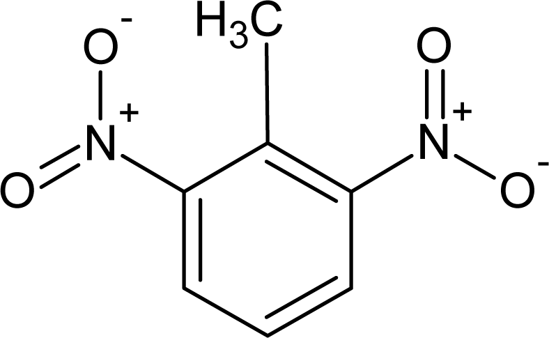 | 606-20-2 | 2,6-Dinitrotoluene |
| 2 | 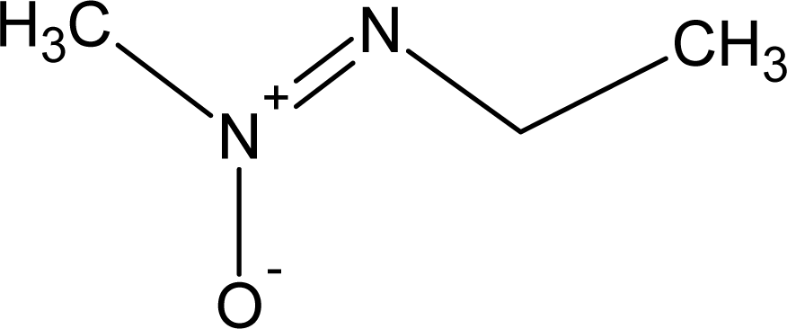 | 57497-34-4 | Z-Methyl-O,N,N-azoxyethane |
| 3 |  | 17608-59-2 | N-Nitrosoephedrine |
| 4 | 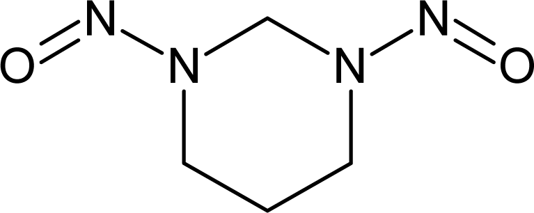 | 15973-99-6 | Di(N-nitroso)-perhydropyrimidine |
| 5 | 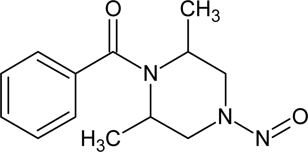 | 61034-40-0 | 1-Nitroso-4-benzoyl-3,5-dimethylpiperazine |
| 6 |  | 99-80-9 | N,4-Dinitrosomethylaniline |
| 7 | 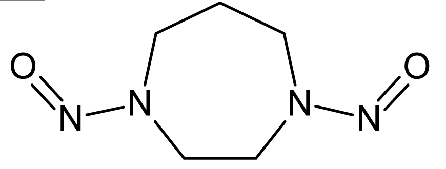 | 55557-00-1 | N,N-Dinitrosohomopiperazine |
| 8 | 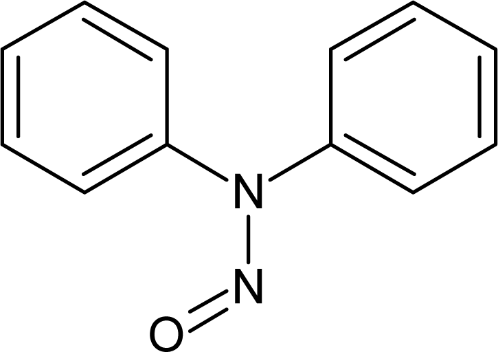 | 86-30-6 | N-Nitrosodiphenylamine |
| 1Sk | CW(1Sk) | 2Sk | CW(2Sk) | dC | CW(dC) |
|---|---|---|---|---|---|
| C........... | −0.0156855 | ||||
| O=C........... | −2.8475657 | O=C.C....... | 0.0 | !-02........ | 1.2190257 |
| [Subtraining-Calibration-Test] system | |||
|---|---|---|---|
| Nepoch | r2subtraining | r2calibration | r2test |
| Split-1 | |||
| 5 | 0.5850 | 0.6043 | 0.5513 |
| 10 | 0.7629 | 0.7675 | 0.7601 |
| 15 | 0.7939 | 0.8006 | 0.7187 |
| 20 | 0.8154 | 0.8243 | 0.6827 |
| 25 | 0.8300 | 0.8262 | 0.6076 |
| Split-2 | |||
| 5 | 0.5947 | 0.6017 | 0.7347 |
| 10 | 0.7195 | 0.7190 | 0.8011 |
| 15 | 0.7551 | 0.7538 | 0.7870 |
| 20 | 0.7732 | 0.7719 | 0.7659 |
| 25 | 0.7839 | 0.7834 | 0.7538 |
| Split-3 | |||
| 5 | 0.6673 | 0.6303 | 0.6548 |
| 10 | 0.7656 | 0.7669 | 0.7519 |
| 15 | 0.8077 | 0.8080 | 0.7205 |
| 20 | 0.8436 | 0.8428 | 0.6288 |
| 25 | 0.8562 | 0.8581 | 0.5503 |
| [Training-Test] system | |||
| Split-1 | |||
| 5 | 0.6255 | 0.6003 | |
| 10 | 0.7761 | 0.7098 | |
| 15 | 0.8124 | 0.6579 | |
| 20 | 0.8386 | 0.5826 | |
| 25 | 0.8521 | 0.5158 | |
| Split-2 | |||
| 5 | 0.6028 | 0.7397 | |
| 10 | 0.7396 | 0.7719 | |
| 15 | 0.7687 | 0.7705 | |
| 20 | 0.7872 | 0.7452 | |
| 25 | 0.7985 | 0.7123 | |
| Split-3 | |||
| 5 | 0.6328 | 0.6559 | |
| 10 | 0.7682 | 0.7127 | |
| 15 | 0.8109 | 0.6397 | |
| 20 | 0.8368 | 0.5378 | |
| 25 | 0.8519 | 0.4573 | |
| SPLIT1 | |||
|---|---|---|---|
| Subtraining set, n=165 | Calibration set, n=167 | Test set, n=61 | SAk distribution |
| [Subtraining-Calibration-Test] system | ||||||||||||
|---|---|---|---|---|---|---|---|---|---|---|---|---|
| limS | Nact | R2 | s | F | R2 | s | F | R2 | s | F | W% | N111 |
| 0 | 797 | 0.8731 | 0.500 | 1125 | 0.8805 | 0.619 | 1217 | 0.5769 | 0.893 | 81 | 42 | 333 |
| 1 | 622 | 0.8807 | 0.485 | 1203 | 0.8821 | 0.621 | 1235 | 0.5319 | 0.942 | 67 | 50 | 314 |
| 2 | 407 | 0.8275 | 0.583 | 783 | 0.8268 | 0.703 | 789 | 0.6305 | 0.832 | 101 | 70 | 285 |
| 3 | 321 | 0.7801 | 0.658 | 579 | 0.7806 | 0.730 | 588 | 0.7102 | 0.732 | 145 | 79 | 255 |
| 4–1 | 266 | 0.7622 | 0.685 | 522 | 0.7620 | 0.734 | 528 | 0.7541 | 0.682 | 181 | 82 | 217 |
| 4–2 | 0.7593 | 0.689 | 514 | 0.7592 | 0.746 | 520 | 0.7483 | 0.692 | 175 | |||
| 4–3 | 0.7643 | 0.682 | 529 | 0.7647 | 0.729 | 536 | 0.7519 | 0.678 | 179 | |||
| average | 0.7619 | 0.685 | 522 | 0.7619 | 0.736 | 528 | 0.7514 | 0.684 | 178 | |||
| 5 | 233 | 0.7247 | 0.737 | 429 | 0.7241 | 0.770 | 433 | 0.7387 | 0.711 | 167 | 85 | 197 |
| 6 | 203 | 0.6901 | 0.781 | 363 | 0.6888 | 0.814 | 365 | 0.7129 | 0.738 | 148 | 86 | 174 |
| 7 | 182 | 0.6704 | 0.806 | 332 | 0.6710 | 0.830 | 337 | 0.6541 | 0.812 | 112 | 84 | 153 |
| 8 | 164 | 0.6528 | 0.827 | 307 | 0.6530 | 0.844 | 311 | 0.7015 | 0.753 | 139 | 87 | 142 |
| 9 | 152 | 0.6356 | 0.847 | 284 | 0.6348 | 0.864 | 287 | 0.6378 | 0.822 | 105 | 84 | 128 |
| 10 | 139 | 0.6178 | 0.868 | 263 | 0.6218 | 0.875 | 271 | 0.6788 | 0.777 | 126 | 84 | 117 |
| Training set, n=332 | Calibration set, n=0 | Test set, n=61 | SAk distribution | |||
| [Training-Test] system | ||||||||||||
|---|---|---|---|---|---|---|---|---|---|---|---|---|
| limS | Nact | R2 | s | F | R2 | s | F | R2 | s | F | W% | N101 |
| 0 | 797 | 0.8868 | 0.472 | 2593 | 0.5429 | 1.002 | 71 | 47 | 376 | |||
| 1 | 777 | 0.8851 | 0.475 | 2542 | 0.5418 | 0.984 | 71 | 46 | 356 | |||
| 2 | 542 | 0.8602 | 0.524 | 2032 | 0.6042 | 0.910 | 91 | 61 | 330 | |||
| 3 | 432 | 0.8313 | 0.576 | 1626 | 0.5575 | 0.917 | 74 | 72 | 309 | |||
| 4 | 385 | 0.8109 | 0.610 | 1417 | 0.5628 | 0.910 | 76 | 75 | 289 | |||
| 5 | 344 | 0.8007 | 0.626 | 1327 | 0.5913 | 0.871 | 86 | 78 | 267 | |||
| 6–1 | 312 | 0.7902 | 0.642 | 1243 | 0.6744 | 0.769 | 122 | 82 | 255 | |||
| 6–2 | 0.7875 | 0.646 | 1223 | 0.7138 | 0.721 | 147 | ||||||
| 6–3 | 0.7843 | 0.651 | 1200 | 0.6947 | 0.744 | 134 | ||||||
| average | 0.7873 | 0.647 | 1222 | 0.6943 | 0.745 | 135 | ||||||
| 7 | 288 | 0.7788 | 0.659 | 1162 | 0.6579 | 0.789 | 114 | 83 | 238 | |||
| 8 | 268 | 0.7659 | 0.678 | 1080 | 0.6677 | 0.777 | 121 | 85 | 227 | |||
| 9 | 246 | 0.7363 | 0.720 | 922 | 0.6853 | 0.757 | 129 | 84 | 207 | |||
| 10 | 234 | 0.7224 | 0.739 | 859 | 0.6909 | 0.750 | 133 | 84 | 196 | |||
| SPLIT2 | |||
|---|---|---|---|
| Subtraining set, n=165 | Calibration set, n=167 | Test set, n=61 | SAk distribution |
| [Subtraining-Calibration-Test] system Split2 | ||||||||||||
|---|---|---|---|---|---|---|---|---|---|---|---|---|
| limS | Nact | R2 | s | F | R2 | s | F | R2 | s | F | W% | N111 |
| 0 | 797 | 0.8743 | 0.507 | 1134 | 0.8737 | 0.540 | 1142 | 0.4630 | 1.055 | 51 | 42 | 337 |
| 1 | 632 | 0.8740 | 0.507 | 1131 | 0.8736 | 0.551 | 1140 | 0.5003 | 0.995 | 59 | 51 | 320 |
| 2 | 425 | 0.8377 | 0.576 | 841 | 0.8367 | 0.580 | 846 | 0.5919 | 0.820 | 86 | 67 | 286 |
| 3 | 335 | 0.8048 | 0.632 | 673 | 0.8041 | 0.633 | 678 | 0.5862 | 0.861 | 84 | 78 | 261 |
| 4 | 284 | 0.7843 | 0.664 | 593 | 0.7842 | 0.663 | 600 | 0.7042 | 0.711 | 141 | 84 | 239 |
| 5 | 247 | 0.7458 | 0.721 | 478 | 0.7448 | 0.728 | 482 | 0.7627 | 0.671 | 190 | 87 | 214 |
| 6–1 | 224 | 0.7315 | 0.741 | 444 | 0.7314 | 0.748 | 449 | 0.7937 | 0.604 | 227 | 84 | 189 |
| 6–2 | 0.7234 | 0.752 | 426 | 0.7234 | 0.760 | 431 | 0.7922 | 0.605 | 225 | |||
| 6–3 | 0.7384 | 0.731 | 460 | 0.7384 | 0.740 | 466 | 0.8136 | 0.593 | 258 | |||
| average | 0.7311 | 0.741 | 444 | 0.7310 | 0.749 | 449 | 0.7998 | 0.600 | 236 | |||
| 7 | 195 | 0.6978 | 0.786 | 376 | 0.7007 | 0.781 | 386 | 0.7318 | 0.657 | 161 | 84 | 164 |
| 8 | 178 | 0.6878 | 0.799 | 359 | 0.6880 | 0.801 | 364 | 0.7223 | 0.682 | 153 | 82 | 146 |
| 9 | 158 | 0.6659 | 0.826 | 325 | 0.6692 | 0.831 | 334 | 0.7104 | 0.709 | 145 | 84 | 133 |
| 10 | 149 | 0.6472 | 0.849 | 299 | 0.6550 | 0.847 | 313 | 0.6970 | 0.723 | 136 | 84 | 125 |
| Training set, n=332 | Calibration set, N=0 | Test set, n=61 | SAk distribution |
| [Training-Test] system Split2 | ||||||||||||
|---|---|---|---|---|---|---|---|---|---|---|---|---|
| limS | Nact | R2 | s | F | R2 | s | F | R2 | s | F | W% | N101 |
| 0 | 797 | 0.8922 | 0.468 | 2734 | 0.4665 | 1.013 | 52 | 47 | 372 | |||
| 1 | 785 | 0.8950 | 0.462 | 2815 | 0.4711 | 1.029 | 53 | 46 | 360 | |||
| 2 | 546 | 0.8740 | 0.506 | 2290 | 0.5329 | 0.887 | 67 | 61 | 335 | |||
| 3 | 442 | 0.8456 | 0.561 | 1807 | 0.5767 | 0.845 | 81 | 71 | 315 | |||
| 4 | 388 | 0.8194 | 0.606 | 1497 | 0.6130 | 0.805 | 94 | 76 | 296 | |||
| 5 | 350 | 0.8122 | 0.618 | 1428 | 0.5802 | 0.873 | 82 | 79 | 278 | |||
| 6 | 321 | 0.8103 | 0.621 | 1412 | 0.6074 | 0.840 | 92 | 83 | 267 | |||
| 7 | 287 | 0.7848 | 0.662 | 1204 | 0.6689 | 0.753 | 120 | 86 | 247 | |||
| 8 | 263 | 0.7594 | 0.700 | 1042 | 0.7345 | 0.655 | 164 | 87 | 229 | |||
| 9–1 | 243 | 0.7397 | 0.728 | 938 | 0.7472 | 0.653 | 174 | 89 | 216 | |||
| 9–2 | 0.7370 | 0.732 | 925 | 0.7862 | 0.602 | 217 | ||||||
| 9–3 | 0.7456 | 0.720 | 967 | 0.7604 | 0.642 | 187 | ||||||
| average | 0.7408 | 0.726 | 943 | 0.7646 | 0.632 | 193 | ||||||
| 10 | 228 | 0.7294 | 0.742 | 890 | 0.7502 | 0.655 | 178 | 86 | 196 | |||
| SPLIT3 | |||
|---|---|---|---|
| Subtraining set, n=165 | Calibration set, n=167 | Test set, n=61 | SAk distribution |
| [Subtraining-Calibration-Test] system Split3 | ||||||||||||
|---|---|---|---|---|---|---|---|---|---|---|---|---|
| limS | Nact | R2 | s | F | R2 | s | F | R2 | s | F | W% | N111 |
| 0 | 797 | 0.8690 | 0.518 | 1084 | 0.8909 | 0.516 | 1353 | 0.5794 | 0.929 | 82 | 42 | 332 |
| 1 | 614 | 0.8742 | 0.508 | 1134 | 0.8946 | 0.513 | 1402 | 0.5995 | 0.896 | 89 | 50 | 309 |
| 2 | 402 | 0.8266 | 0.597 | 778 | 0.8331 | 0.614 | 826 | 0.6748 | 0.800 | 122 | 69 | 278 |
| 3–1 | 324 | 0.7963 | 0.647 | 637 | 0.7982 | 0.633 | 652 | 0.7176 | 0.729 | 150 | 78 | 254 |
| 3–2 | 0.7919 | 0.654 | 620 | 0.7937 | 0.639 | 635 | 0.6969 | 0.758 | 136 | |||
| 3–3 | 0.7930 | 0.652 | 624 | 0.7944 | 0.641 | 637 | 0.7431 | 0.698 | 171 | |||
| average | 0.7937 | 0.651 | 627 | 0.7954 | 0.638 | 642 | 0.7192 | 0.728 | 152 | |||
| 4 | 264 | 0.7439 | 0.725 | 474 | 0.7462 | 0.703 | 485 | 0.6992 | 0.765 | 138 | 85 | 224 |
| 5 | 227 | 0.7127 | 0.768 | 404 | 0.7136 | 0.738 | 411 | 0.6900 | 0.774 | 133 | 86 | 195 |
| 6 | 198 | 0.6945 | 0.792 | 371 | 0.7013 | 0.756 | 388 | 0.6899 | 0.770 | 133 | 86 | 171 |
| 7 | 181 | 0.6790 | 0.812 | 345 | 0.6843 | 0.780 | 358 | 0.6995 | 0.758 | 137 | 85 | 154 |
| 8 | 159 | 0.6432 | 0.856 | 294 | 0.6493 | 0.815 | 306 | 0.7061 | 0.749 | 142 | 84 | 134 |
| 9 | 147 | 0.6219 | 0.881 | 268 | 0.6533 | 0.820 | 311 | 0.6934 | 0.775 | 134 | 84 | 123 |
| 10 | 140 | 0.5952 | 0.911 | 240 | 0.6269 | 0.849 | 277 | 0.6300 | 0.842 | 101 | 83 | 116 |
| Training set, n=332 | Calibration set, n=0 | Test set, n=61 | SAk distribution |
| [Training-Test] system Split3 | ||||||||||||
|---|---|---|---|---|---|---|---|---|---|---|---|---|
| limS | Nact | R2 | s | F | R2 | s | F | R2 | s | F | W% | N101 |
| 0 | 797 | 0.8930 | 0.457 | 2756 | 0.5532 | 1.009 | 73 | 47 | 377 | |||
| 1 | 776 | 0.8932 | 0.457 | 2763 | 0.5529 | 0.996 | 73 | 46 | 356 | |||
| 2 | 540 | 0.8699 | 0.504 | 2209 | 0.5998 | 0.922 | 89 | 61 | 327 | |||
| 3 | 434 | 0.8349 | 0.568 | 1674 | 0.5908 | 0.896 | 88 | 72 | 311 | |||
| 4 | 388 | 0.8220 | 0.590 | 1528 | 0.6068 | 0.865 | 92 | 75 | 291 | |||
| 5 | 348 | 0.8030 | 0.620 | 1346 | 0.6650 | 0.796 | 117 | 78 | 272 | |||
| 6–1 | 320 | 0.7773 | 0.660 | 1152 | 0.7017 | 0.751 | 139 | 82 | 261 | |||
| 6–2 | 0.7942 | 0.634 | 1273 | 0.6967 | 0.761 | 136 | ||||||
| 6–3 | 0.7834 | 0.651 | 1193 | 0.7171 | 0.735 | 150 | ||||||
| average | 0.7850 | 0.648 | 1206 | 0.7051 | 0.749 | 141 | ||||||
| 7 | 288 | 0.7598 | 0.685 | 1045 | 0.6807 | 0.778 | 126 | 84 | 241 | |||
| 8 | 271 | 0.7637 | 0.679 | 1067 | 0.6520 | 0.817 | 112 | 85 | 229 | |||
| 9 | 244 | 0.7318 | 0.724 | 901 | 0.6833 | 0.778 | 127 | 86 | 210 | |||
| 10 | 232 | 0.7288 | 0.728 | 887 | 0.6826 | 0.781 | 127 | 84 | 196 | |||
| SMILES-Attributes (SA) | CW(SA) probe 1 | CW(SA) probe 2 | CW(SA) probe 3 | N(Subtr) | N(Calib) | N(Test) |
|---|---|---|---|---|---|---|
| dC | ||||||
| !-01........ | 2.7522274 | 2.8704615 | 3.5346711 | 5 | 4 | 0 |
| !-02........ | 1.2190257 | 2.1277910 | 1.8790680 | 10 | 9 | 3 |
| !-03........ | 6.6784389 | 8.0311759 | 7.1271958 | 15 | 10 | 3 |
| !-04........ | 1.4326102 | 1.6702225 | 1.9340790 | 17 | 22 | 8 |
| !-05........ | 3.9671055 | 4.0344924 | 4.1729635 | 9 | 11 | 6 |
| !-06........ | 5.8564637 | 5.8794012 | 6.4409754 | 8 | 11 | 7 |
| !-07........ | 5.4970475 | 5.1611240 | 5.2308474 | 5 | 3 | 0 |
| !-08........ | 9.1295923 | 9.5122328 | 9.0035813 | 4 | 3 | 1 |
| !-21........ | −1.6383248 | 1.8781962 | 0.0037831 | 4 | 0 | 0 |
| !000........ | 3.6271821 | 4.6894405 | 3.7495506 | 6 | 7 | 1 |
| !002........ | 1.5603260 | 1.7450611 | 1.4951171 | 4 | 4 | 1 |
| !003........ | −1.2514096 | −1.3248590 | −1.1256941 | 5 | 8 | 2 |
| !004........ | 0.7359726 | 1.0643522 | 1.2450258 | 11 | 8 | 1 |
| !005........ | 0.9702817 | 0.6240636 | 1.2144260 | 13 | 9 | 4 |
| !006........ | 4.1543029 | 4.9338830 | 4.9975361 | 7 | 5 | 2 |
| !007........ | −3.7770327 | −3.5039029 | −3.0945823 | 4 | 3 | 3 |
| !010........ | 0.5049355 | −0.2636435 | 0.3157527 | 6 | 8 | 3 |
| !012........ | 3.2511213 | 3.2471578 | 4.5049864 | 6 | 3 | 1 |
| 1SAk | ||||||
| #........... | 3.3706294 | 3.3739877 | 2.0643948 | 5 | 3 | 0 |
| (........... | −1.6866726 | −1.3666396 | −1.5485382 | 708 | 780 | 260 |
| /........... | −0.4913426 | 0.1880630 | −1.0975733 | 17 | 24 | 4 |
| 1........... | −1.4970879 | −0.8440743 | −0.0771659 | 222 | 222 | 88 |
| 2........... | −0.1050677 | −1.1891334 | −1.1138329 | 130 | 132 | 48 |
| 3........... | −1.3433340 | 0.0456678 | −0.1828115 | 60 | 60 | 20 |
| 4........... | 3.4954870 | 3.1562107 | 3.5453447 | 20 | 18 | 8 |
| 5........... | 2.8128037 | 3.3899959 | 1.6902086 | 10 | 10 | 4 |
| =........... | −1.8660845 | −2.1441609 | −1.8865449 | 77 | 79 | 23 |
| C........... | −0.0156855 | 0.0453525 | 0.2198595 | 765 | 736 | 290 |
| Br.......... | 0.5327181 | 0.2779344 | 0.8454938 | 23 | 8 | 1 |
| Cl.......... | 2.9838590 | 2.1906970 | 3.1890603 | 61 | 85 | 13 |
| F........... | −0.4680666 | −1.0425952 | 0.2836492 | 15 | 19 | 8 |
| O=C......... | −2.8475657 | −2.4376628 | −2.9332073 | 33 | 21 | 13 |
| O=.......... | 0.7369372 | 0.0037805 | 1.4086398 | 140 | 132 | 47 |
| N........... | 1.1227501 | 1.1982965 | 1.4193640 | 196 | 201 | 76 |
| O........... | −1.2649109 | −0.4408418 | −0.1501499 | 138 | 143 | 45 |
| S........... | 2.3712714 | 2.6251760 | 2.5313565 | 13 | 12 | 7 |
| [N+]........ | 1.9345689 | 1.6543771 | 3.0457447 | 26 | 31 | 12 |
| [O−]........ | 5.9250900 | 5.6230564 | 6.9653600 | 26 | 32 | 12 |
| [........... | −2.1531745 | −2.8080919 | −1.9966710 | 4 | 6 | 0 |
| \........... | 3.3565892 | 3.4338813 | 2.9027414 | 14 | 29 | 7 |
| c........... | −0.0357264 | 0.0373181 | 0.0419142 | 653 | 679 | 247 |
| n........... | −0.6564241 | −0.1251570 | −1.4184164 | 37 | 44 | 23 |
| o........... | −1.0665085 | −1.3777640 | −0.2485470 | 16 | 12 | 7 |
| s........... | −0.0527175 | −0.9991370 | −1.0040993 | 7 | 6 | 7 |
| 2SAk | ||||||
| (...(....... | −0.0735964 | −0.1751550 | −0.4970432 | 18 | 28 | 4 |
| /...(....... | −0.9972903 | −1.5270762 | −0.7479799 | 7 | 10 | 2 |
| 1...(....... | 2.3733452 | 2.4975765 | 2.4084744 | 37 | 45 | 15 |
| 2...(....... | 0.0608136 | 0.1227718 | −0.1848792 | 14 | 15 | 6 |
| 2...1....... | 5.7529509 | 6.6287931 | 7.4713129 | 5 | 6 | 2 |
| 3...(....... | −1.6283079 | −0.2528134 | −2.0499858 | 6 | 3 | 0 |
| 3...2....... | −1.5915226 | −1.5268568 | −1.9365673 | 4 | 6 | 3 |
| =...(....... | 1.8468333 | 2.3079839 | 2.4377851 | 14 | 17 | 3 |
| =...1....... | 2.5039102 | −0.5608527 | −0.0325572 | 7 | 5 | 1 |
| =...2....... | −3.2847055 | −2.5042239 | −2.0658154 | 7 | 5 | 2 |
| =...3....... | 3.4389111 | 0.8278003 | 3.5625409 | 6 | 5 | 4 |
| C...#....... | −0.1836222 | −0.9385750 | −0.4107562 | 6 | 3 | 0 |
| C...(....... | −0.7573851 | 0.0280162 | 0.7466835 | 443 | 456 | 163 |
| C.../....... | 1.1245359 | 0.0042443 | 0.8873189 | 13 | 13 | 2 |
| C...1....... | −0.4566262 | 0.0357389 | −1.3911620 | 74 | 73 | 30 |
| C...2....... | 0.3115003 | 1.0911890 | 0.8401947 | 46 | 47 | 12 |
| C...3....... | 3.6534836 | 3.4678053 | 2.9866499 | 40 | 22 | 8 |
| C...4....... | −0.7152591 | −0.7967591 | −1.2502575 | 17 | 13 | 5 |
| C...5....... | 3.6909807 | 4.4229382 | 4.3015822 | 10 | 7 | 6 |
| C...=....... | −0.5319093 | −0.5807285 | −0.4569253 | 98 | 101 | 29 |
| C...C....... | −0.4098212 | −0.6663667 | −0.4722713 | 244 | 211 | 113 |
| Br..(....... | −1.2467411 | −0.7804139 | −0.9676602 | 24 | 7 | 0 |
| Br..C....... | 5.8039394 | 6.6601591 | 5.9721683 | 9 | 5 | 1 |
| Cl..(....... | −0.2165917 | −0.6443513 | −0.7389015 | 68 | 104 | 11 |
| Cl..C....... | 6.8768666 | 7.6839570 | 7.4343341 | 17 | 18 | 5 |
| F...(....... | 0.2020867 | −0.0538118 | −0.1868874 | 24 | 22 | 12 |
| O=C.(....... | 0.7311485 | −1.6257029 | 0.2188934 | 18 | 8 | 5 |
| O=C.1....... | 4.3778160 | 4.7809340 | 4.0011131 | 9 | 6 | 1 |
| O=..(....... | −0.5612999 | −1.5272716 | −1.1454337 | 177 | 158 | 60 |
| O=..1....... | −2.5019413 | −3.3715192 | −4.0028237 | 4 | 2 | 0 |
| N...#....... | −3.8725309 | −4.4992215 | −3.7843832 | 4 | 2 | 0 |
| N...(....... | 0.0666245 | 0.7453778 | −0.1289674 | 140 | 165 | 56 |
| N.../....... | 0.8133323 | 0.0606093 | −0.1893841 | 9 | 12 | 2 |
| N...1....... | 1.8744868 | 1.0335496 | 1.5038557 | 23 | 17 | 10 |
| N...2....... | 1.4979132 | 1.4959901 | 1.4961647 | 6 | 9 | 3 |
| N...=....... | −1.3157419 | 0.1537739 | −0.3882898 | 12 | 16 | 5 |
| N...C....... | 1.4051238 | 0.9827410 | 1.0619180 | 63 | 70 | 24 |
| N...O=...... | 6.1270291 | 7.3000058 | 4.8170313 | 39 | 34 | 13 |
| N...N....... | 3.1922498 | 3.5013150 | 4.1321688 | 14 | 8 | 8 |
| O...(....... | −0.1195150 | −0.1976562 | −0.7838811 | 106 | 111 | 31 |
| O...1....... | −0.7620380 | −1.4388311 | −1.9361803 | 19 | 13 | 5 |
| O...2....... | −2.5618134 | −3.2668394 | −2.8747322 | 9 | 5 | 3 |
| O...C....... | 1.0444154 | 1.0339726 | 0.9105754 | 90 | 96 | 29 |
| S...(....... | −0.7479741 | 0.4990928 | −0.0132133 | 7 | 8 | 4 |
| S...=....... | 1.5009045 | 0.6752299 | −0.2807681 | 5 | 7 | 2 |
| S...C....... | 0.2470117 | −1.2535030 | −0.5349209 | 6 | 1 | 4 |
| [N+](....... | 3.2516821 | 1.6524330 | 1.3748828 | 40 | 37 | 17 |
| [O−](....... | −0.4532482 | −0.8221590 | −1.3547359 | 39 | 48 | 18 |
| [O−][N+].... | 0.2616708 | 0.6284804 | −1.2536848 | 5 | 6 | 2 |
| \...(....... | 0.2506876 | −0.8700648 | −1.1268254 | 5 | 11 | 1 |
| \...C....... | 2.1710329 | 2.6262343 | 1.7619375 | 11 | 26 | 6 |
| \...N....... | −3.1201815 | −3.8706242 | −3.0325970 | 4 | 12 | 3 |
| c...(....... | 0.3275817 | −0.1910585 | −0.5343311 | 183 | 238 | 94 |
| c...1....... | 0.5127781 | 0.1714980 | 0.8236519 | 196 | 204 | 75 |
| c...2....... | 0.1139969 | 1.4331593 | 2.2509927 | 129 | 122 | 38 |
| c...3....... | 1.5045372 | 1.4375414 | 0.1592669 | 41 | 50 | 15 |
| c...4....... | 0.9391582 | 0.2451376 | 0.7605772 | 9 | 10 | 10 |
| c...C....... | −1.6459258 | 0.0580657 | −0.4333240 | 15 | 19 | 1 |
| c...Cl...... | −1.9973422 | −2.7517912 | −3.6905785 | 5 | 7 | 3 |
| c...N....... | 1.0896408 | 0.1897391 | 0.7548234 | 26 | 19 | 12 |
| c...O....... | 2.4331156 | 1.2515997 | 0.9178503 | 22 | 18 | 6 |
| c...c....... | −0.2252497 | −0.6284915 | −0.8624749 | 316 | 305 | 106 |
| n...(....... | 0.8765637 | −0.9401023 | 0.2494319 | 11 | 8 | 6 |
| n...1....... | 1.6235455 | 1.2765370 | 1.8586068 | 16 | 15 | 10 |
| n...2....... | 2.0303385 | 3.9797145 | 3.5009942 | 6 | 11 | 8 |
| n...3....... | 4.1295873 | 3.5576218 | 4.1220666 | 4 | 6 | 3 |
| n...c....... | 2.3101715 | 1.5599987 | 1.7164852 | 25 | 40 | 17 |
| o...(....... | −3.9990305 | −2.9953875 | −3.7613936 | 8 | 9 | 6 |
| o...1....... | 5.8875962 | 7.1857177 | 6.8437068 | 5 | 5 | 2 |
| o...2....... | −0.6199000 | −0.1044473 | −0.2658548 | 7 | 6 | 5 |
| o...c....... | 5.5725605 | 4.2549084 | 3.0289124 | 8 | 3 | 1 |
| s...1....... | 0.9407152 | 1.9765325 | 2.0040980 | 6 | 6 | 7 |
| s...c....... | −0.4960014 | 0.0005352 | 0.0003709 | 4 | 2 | 6 |
| 3SAk | ||||||
| (...C...(... | 3.9980286 | 3.5630634 | 2.4208800 | 95 | 102 | 42 |
| (...Br..(... | 0.0004754 | 0.5262619 | −1.7321140 | 9 | 3 | 0 |
| (...Cl..(... | 0.6233843 | −0.3777470 | 1.3569611 | 29 | 44 | 5 |
| (...F...(... | 1.9216525 | 2.4994253 | 1.1337512 | 11 | 9 | 5 |
| (...O=..(... | 1.2586684 | 0.9193678 | 0.2775945 | 71 | 68 | 28 |
| (...N...(... | 2.1549141 | 1.5500875 | 1.3741232 | 29 | 40 | 11 |
| (...O...(... | 1.3921586 | 0.5590769 | 0.3741692 | 33 | 34 | 8 |
| (...[N+](... | 2.2543551 | 4.4491588 | 4.0323477 | 15 | 8 | 5 |
| (...[O−](... | −1.5354823 | −1.4737180 | −3.3779724 | 19 | 23 | 9 |
| (...c...(... | −1.0930229 | −0.9342219 | 0.4332127 | 12 | 18 | 0 |
| /...C...(... | 4.4970818 | 4.0048287 | 3.0000737 | 5 | 4 | 0 |
| 1...C...(... | 4.2142525 | 2.8161885 | 3.1850279 | 16 | 16 | 5 |
| 1...O...(... | 2.2528410 | 0.3797661 | 1.4952742 | 4 | 2 | 0 |
| 1...c...(... | 0.9335129 | 0.5288083 | 0.8716499 | 18 | 35 | 12 |
| 2...C...(... | −2.2544539 | −1.0919167 | −2.6427067 | 10 | 13 | 4 |
| 2...c...(... | 2.9972422 | 3.4417285 | 3.8400379 | 29 | 28 | 12 |
| 2...c...1... | 1.9960734 | 0.5619955 | −0.0932258 | 7 | 8 | 2 |
| 2...o...(... | 1.0110528 | 1.4973281 | 1.0603210 | 4 | 4 | 4 |
| 3...C...(... | −2.2814415 | −2.8156671 | −1.9977117 | 7 | 6 | 1 |
| 3...C...2... | 6.4980735 | 8.0020020 | 8.2529271 | 4 | 0 | 0 |
| 3...c...(... | −0.2171379 | 1.0578016 | 1.2483687 | 9 | 9 | 4 |
| 3...c...2... | 5.2502023 | 4.2226554 | 4.7487134 | 8 | 7 | 2 |
| 4...C...(... | 1.7464204 | −0.6210801 | −0.2842473 | 6 | 4 | 0 |
| =...C...3... | 7.0029958 | 7.5641676 | 6.7549811 | 8 | 4 | 0 |
| =...C...1... | 2.9999456 | 2.8474909 | 4.2545986 | 12 | 8 | 4 |
| =...C...(... | 1.5713076 | 0.9521538 | 0.5309943 | 18 | 18 | 2 |
| =...C.../... | 5.2495800 | 5.4994084 | 6.0049990 | 6 | 7 | 2 |
| =...N.../... | 5.8119346 | 5.5954944 | 6.3789368 | 7 | 8 | 2 |
| C...(...C... | 0.5513380 | −0.2378199 | −1.0864076 | 69 | 64 | 24 |
| C...(...1... | −1.1216831 | −3.3768328 | −2.4951909 | 9 | 10 | 3 |
| C...(...=... | 6.2535976 | 5.1587497 | 4.4360925 | 9 | 11 | 3 |
| C...(...(... | −0.3146880 | −1.6918223 | −1.2834724 | 11 | 22 | 3 |
| C.../...(... | −3.0637430 | −1.8160468 | −2.9987839 | 5 | 4 | 1 |
| C...1...C... | 5.4954661 | 3.9189550 | 4.6140280 | 8 | 10 | 5 |
| C...1...(... | 1.3718529 | 1.3079333 | 1.4795097 | 8 | 13 | 1 |
| C...1...=... | 0.2476856 | 1.3169467 | 0.9333222 | 6 | 4 | 1 |
| C...2...(... | −0.6449419 | −0.8430901 | −0.7370108 | 5 | 9 | 0 |
| C...2...C... | 5.9965379 | 5.9966533 | 6.0017257 | 8 | 6 | 1 |
| C...2...=... | 0.0028591 | −0.8747150 | −0.3764369 | 7 | 5 | 2 |
| C...3...(... | 6.5045056 | 6.2477966 | 5.7492216 | 5 | 3 | 0 |
| C...3...=... | 5.6231609 | 6.0002916 | 5.1293498 | 5 | 3 | 2 |
| C...3...C... | −3.5000076 | −2.9954231 | −3.0028309 | 11 | 2 | 3 |
| C...4...C... | −3.0021372 | −4.5016046 | −2.9968826 | 4 | 1 | 1 |
| C...=...1... | 0.4331526 | 2.6582434 | 1.9050556 | 7 | 5 | 1 |
| C...=...(... | −2.4953051 | −0.6283873 | −0.7473193 | 8 | 11 | 1 |
| C...=...C... | 1.6093540 | 2.7975919 | 2.1897927 | 33 | 34 | 11 |
| C...=...3... | 0.2971809 | 1.5013043 | −0.9639603 | 5 | 3 | 2 |
| C...=...2... | 1.6275637 | 3.7172258 | 1.7773288 | 7 | 4 | 0 |
| C...C...3... | 5.0746157 | 4.6119002 | 4.5908880 | 16 | 8 | 5 |
| C...C...=... | −0.4018420 | −1.0583619 | −1.0977818 | 36 | 26 | 5 |
| C...C...1... | 1.8775937 | 0.9384077 | 1.3828674 | 31 | 27 | 17 |
| C...C...2... | 0.7079969 | −0.1879112 | 0.6274962 | 21 | 19 | 3 |
| C...C...(... | 1.0123078 | 0.7924398 | 0.4047303 | 109 | 109 | 42 |
| C...C...4... | −1.4024533 | −0.7803070 | −0.3715353 | 7 | 5 | 2 |
| C...C...C... | −0.0428402 | 0.1882515 | −0.1515135 | 77 | 58 | 59 |
| C...Br..(... | 1.6298040 | 2.5038504 | 1.0267176 | 4 | 1 | 0 |
| C...Cl..(... | −1.4962815 | −0.4993582 | −1.2516847 | 4 | 4 | 1 |
| C...N...1... | −0.2691219 | −0.3795019 | −1.0000894 | 8 | 8 | 1 |
| C...N...(... | 1.4422504 | 0.9731136 | 0.4339815 | 36 | 35 | 18 |
| C...O...2... | 5.1236472 | 4.0895698 | 3.5121038 | 5 | 3 | 1 |
| C...O...(... | 3.2515162 | 2.2843408 | 2.5780816 | 28 | 32 | 12 |
| C...O...C... | 4.3741698 | 4.3105041 | 3.0634685 | 8 | 10 | 4 |
| C...O...1... | 2.8733789 | 3.1267319 | 2.9673439 | 13 | 9 | 3 |
| C...\...C... | −2.8461979 | −3.8759584 | −2.2789129 | 4 | 8 | 1 |
| C...c...2... | 6.0006860 | 4.5315715 | 5.2468516 | 4 | 5 | 0 |
| C...c...1... | 2.4356912 | 0.4351720 | 1.2472872 | 10 | 13 | 1 |
| Br..(...C... | 2.0615855 | 1.1437599 | 1.9040185 | 4 | 6 | 0 |
| Br..C...(... | 1.4981969 | 0.6256406 | 0.0009660 | 7 | 3 | 0 |
| Cl..(...(... | −1.2075807 | −0.6362162 | −1.9255180 | 9 | 6 | 0 |
| Cl..(...C... | −1.1526609 | −0.2476848 | −1.8147825 | 27 | 32 | 4 |
| Cl..(...Cl.. | 0.5049208 | 3.2539441 | 0.6886852 | 4 | 7 | 0 |
| Cl..C...C... | −0.0014586 | 0.0039516 | −1.2464369 | 9 | 10 | 2 |
| Cl..c...1... | −0.2533902 | 1.6295626 | 2.2512123 | 4 | 6 | 3 |
| F...(...C... | 1.6863754 | 1.5015167 | 0.5346605 | 5 | 8 | 2 |
| F...(...(... | −1.7457403 | −2.1139078 | −1.1982770 | 6 | 8 | 4 |
| O=C.1...C... | 5.1279970 | 2.8669862 | 3.6914477 | 4 | 3 | 1 |
| O=..(...C... | 0.8107109 | 0.7780984 | −0.4033174 | 92 | 68 | 31 |
| O=..1...C... | −3.7510578 | −4.1255552 | −4.1222938 | 4 | 2 | 0 |
| O=..N...(... | 9.5435183 | 10.0636543 | 10.0315899 | 24 | 28 | 6 |
| N...#...C... | −4.5000318 | −4.5014930 | −4.5004055 | 4 | 1 | 0 |
| N...(...N... | 1.1916803 | 0.9983579 | 1.6288201 | 12 | 10 | 2 |
| N...(...1... | −0.1264931 | −0.7538114 | 0.0454142 | 5 | 7 | 0 |
| N...(...C... | 3.5018836 | 2.2822748 | 3.0336305 | 55 | 62 | 30 |
| N...(...O=.. | −2.3138510 | −2.3145054 | −1.5031092 | 23 | 14 | 5 |
| N...(...O=C. | −1.4990141 | −0.8704228 | −1.2494712 | 6 | 5 | 2 |
| N...1...C... | 2.6914072 | 2.5647275 | 2.7184638 | 12 | 13 | 4 |
| N...2...C... | −0.4978517 | −0.0000051 | 1.0021092 | 5 | 6 | 1 |
| N...C...(... | −0.8104915 | −0.4341890 | −0.9684013 | 25 | 24 | 8 |
| N...C...C... | −1.2520104 | −0.7226801 | −1.0008159 | 22 | 26 | 6 |
| N...O=..(... | 2.6715972 | 1.6272171 | 3.6550784 | 11 | 11 | 1 |
| N...N...1... | 0.0042593 | 1.4970138 | 1.1825822 | 5 | 3 | 3 |
| N...N...O=.. | 4.2459870 | 3.7466101 | 3.2221499 | 10 | 6 | 5 |
| N...N...(... | 4.7536740 | 5.4055258 | 4.6294702 | 6 | 4 | 2 |
| N...c...2... | −3.6269860 | −2.8792235 | −4.2532265 | 5 | 3 | 1 |
| N...c...1... | −0.1899251 | 0.2338572 | 0.2627307 | 20 | 15 | 11 |
| O...(...O=.. | −0.6219316 | 1.4395827 | 1.2532594 | 19 | 17 | 5 |
| O...(...C... | 0.9395840 | −0.4347300 | 0.4467587 | 52 | 40 | 17 |
| O...(...(... | 11.5040533 | 12.0049318 | 11.9989881 | 4 | 4 | 1 |
| O...(...O=C. | 4.9368982 | 4.9994000 | 4.7472261 | 7 | 2 | 0 |
| O...C...1... | −0.4987416 | 0.4978181 | 0.9413176 | 4 | 4 | 3 |
| O...C...C... | −2.6559832 | −3.2412835 | −3.2024047 | 35 | 37 | 10 |
| O...C...(... | −0.1201364 | −0.3106109 | −1.2477221 | 27 | 31 | 10 |
| O...c...1... | −2.7623334 | −2.0920952 | −2.1242060 | 14 | 8 | 3 |
| O...c...2... | −1.4980614 | −3.5286748 | −3.6223778 | 7 | 6 | 0 |
| S...C...C... | −0.0034408 | 1.5042803 | 0.7537994 | 4 | 0 | 2 |
| [N+](...C... | 9.2539066 | 9.4417355 | 7.5006239 | 6 | 4 | 1 |
| [N+](...2... | 5.4109375 | 4.6273127 | 3.2821267 | 6 | 3 | 4 |
| [N+](...O=.. | −0.3787790 | 0.3109436 | 0.1872916 | 4 | 7 | 2 |
| [O−](...[N+] | −3.8743809 | −1.4388021 | −1.2453181 | 18 | 22 | 9 |
| [O−](...O=.. | −4.0585677 | −2.6242009 | −2.5577359 | 15 | 11 | 6 |
| [O−][N+](... | −3.5045096 | −1.4982980 | −2.4892797 | 5 | 5 | 2 |
| \...C...=... | −1.3136029 | −1.8755430 | −1.2854492 | 4 | 11 | 1 |
| \...C...(... | −3.5018378 | −4.4994516 | −3.8096741 | 5 | 7 | 2 |
| c...(...[O−] | 3.9992170 | 4.0612326 | 4.4978479 | 4 | 10 | 3 |
| c...(...c... | 1.7523875 | 2.5921235 | 0.9359654 | 24 | 19 | 13 |
| c...(...Br.. | 1.3392341 | 0.5340779 | 1.1889034 | 17 | 0 | 0 |
| c...(...C... | 1.0002010 | 0.2472155 | −0.2478234 | 19 | 41 | 13 |
| c...(...Cl.. | 1.1825597 | 2.5039425 | 0.9088978 | 15 | 23 | 7 |
| c...(...O... | 1.1553993 | 0.9107402 | 1.8401083 | 10 | 34 | 6 |
| c...(...N... | −0.4647652 | −0.5109250 | 0.5049629 | 13 | 41 | 11 |
| c...(...1... | 3.2546395 | 1.6826438 | 1.7521385 | 17 | 17 | 10 |
| c...(...O=.. | 2.0008786 | 2.9044603 | 2.8172049 | 15 | 17 | 7 |
| c...(...F... | 2.5615727 | 2.2483847 | 2.9956341 | 6 | 0 | 2 |
| c...1...O... | 0.3157218 | 0.2460029 | 0.0026575 | 7 | 3 | 3 |
| c...1...C... | −0.3426326 | −0.4053179 | −0.0587013 | 10 | 10 | 4 |
| c...1...(... | 4.1291472 | 3.7385617 | 4.5010102 | 15 | 17 | 6 |
| c...1...c... | 2.5270201 | 4.1254591 | 1.6392878 | 64 | 69 | 24 |
| c...2...c... | 3.1834674 | 3.5765233 | 2.5649848 | 46 | 41 | 10 |
| c...2...O... | −2.1902681 | −0.8169002 | −1.5600959 | 6 | 5 | 0 |
| c...2...C... | 2.0599980 | 3.3166075 | 2.0508240 | 6 | 4 | 2 |
| c...2...(... | −3.4837706 | −2.7454921 | −2.2497303 | 5 | 2 | 2 |
| c...3...c... | 0.5671953 | 0.3280375 | 2.5577465 | 14 | 15 | 6 |
| c...C...C... | −0.4968006 | −1.0630716 | −0.7464899 | 4 | 6 | 0 |
| c...N...(... | 4.1212930 | 5.1280879 | 3.2342653 | 9 | 3 | 3 |
| c...O...(... | 7.8795041 | 8.7529500 | 8.5448576 | 5 | 2 | 0 |
| c...O...C... | 0.4969760 | 1.0602889 | 1.0035994 | 10 | 8 | 0 |
| c...c...2... | −1.0046754 | −0.7477295 | −1.3148992 | 59 | 58 | 20 |
| c...c...c... | −0.9189229 | −1.1362229 | −0.9886103 | 171 | 148 | 50 |
| c...c...1... | 0.9684404 | 1.0961687 | 1.0267859 | 111 | 101 | 36 |
| c...c...3... | −1.4056269 | −2.8661586 | −1.7490548 | 18 | 24 | 6 |
| c...c...4... | −1.2498300 | 0.6278968 | 0.4997288 | 5 | 5 | 4 |
| c...c...(... | −0.5592802 | −0.7452834 | −0.2831183 | 87 | 110 | 45 |
| c...n...1... | 0.4037274 | 0.7545182 | 1.8635708 | 8 | 9 | 8 |
| n...1...c... | 1.1446162 | 1.1906216 | 0.1368885 | 11 | 8 | 8 |
| n...c...c... | −4.4951810 | −4.4955509 | −4.2500468 | 5 | 11 | 1 |
| n...c...(... | −1.7475062 | −0.9098866 | −0.0016730 | 10 | 13 | 13 |
| o...(...c... | 1.9983265 | −0.3077248 | 1.1610603 | 5 | 5 | 5 |
| o...1...(... | −0.8795536 | −0.8151611 | −1.4961309 | 4 | 3 | 2 |
| s...1...(... | 3.0007359 | 3.3126224 | 2.8719278 | 5 | 5 | 6 |
| Structure | CAS and SMILES | logTD50 |
|---|---|---|
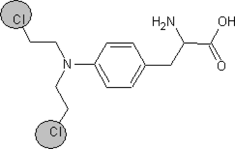 | 148-82-3
O=C(O)C(N)Cc1ccc(cc1)N(CCCl)CCCl | 3.512 |
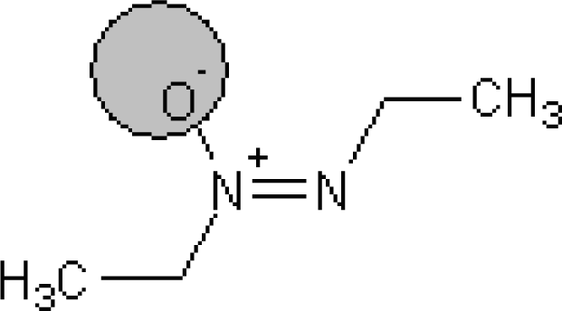 | 16301-26-1
[O−]\[N+](CC)=N\CC | 3.667 |
 | 1163-19-5
Brc2c(Oc1c(Br)c(Br)c(Br)c(Br)c1Br)c(Br)c(Br)c(Br)c2Br | −0.542* |
 | 91-93-0
COc1cc(ccc1/N=C=O)c2ccc(\N=C=O)c(OC)c2 | −0.740* |
© 2009 by the authors; licensee Molecular Diversity Preservation International, Basel, Switzerland. This article is an open-access article distributed under the terms and conditions of the Creative Commons Attribution license (http://creativecommons.org/licenses/by/3.0/).
Share and Cite
Toropov, A.A.; Toropova, A.P.; Benfenati, E. Additive SMILES-Based Carcinogenicity Models: Probabilistic Principles in the Search for Robust Predictions. Int. J. Mol. Sci. 2009, 10, 3106-3127. https://doi.org/10.3390/ijms10073106
Toropov AA, Toropova AP, Benfenati E. Additive SMILES-Based Carcinogenicity Models: Probabilistic Principles in the Search for Robust Predictions. International Journal of Molecular Sciences. 2009; 10(7):3106-3127. https://doi.org/10.3390/ijms10073106
Chicago/Turabian StyleToropov, Andrey A., Alla P. Toropova, and Emilio Benfenati. 2009. "Additive SMILES-Based Carcinogenicity Models: Probabilistic Principles in the Search for Robust Predictions" International Journal of Molecular Sciences 10, no. 7: 3106-3127. https://doi.org/10.3390/ijms10073106