Composition-Dependent Dielectric Properties of DMF-Water Mixtures by Molecular Dynamics Simulations

Abstract
:1. Introduction
2. Methodology
2.1. Force fielids and simulation details
3. Results and Discussion
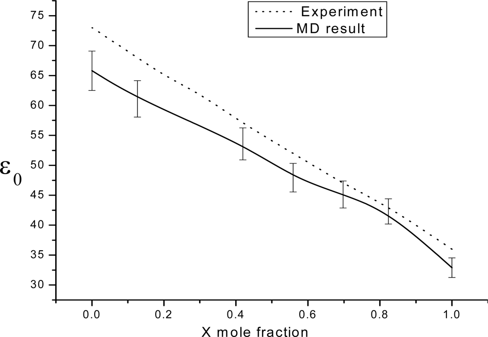
3.1. Theoretical framework
4. Dynamic Dielectric Properties
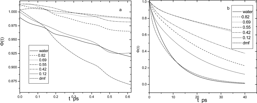
4.1. Dipole density time correlations
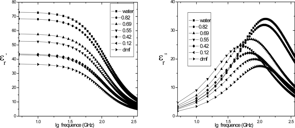
4.2. Dielectric relaxation
5. Summary
Acknowledgments
References and Notes
- Lampreia, I; Magalhaes, S; Rodrigues, S; Mendonca, A. Solubility of proline–leucine dipeptide in water and in aqueous sodium chloride solutions from T = (288.15 to 313.15) K. J.Chem. Thermodyn 2006, 38, 240–244. [Google Scholar]
- de la Hoz, A; Díaz-Ortiz, Á; Moreno, A. Microwaves in organic synthesis. Thermal and nonthermal microwave effects. Chem. Soc. Rev 2005, 34, 164–178. [Google Scholar]
- Pieter, AC; Quist, JS; Marc, MK; Tom, JS; Laurens, DAS. Formation and decay of charge carriers in bulk heterojunctions of MDMO-PPV or P3HT with new n-type conjugated polymers. J. Phys. Chem. C 2007, 111, 4452–4457. [Google Scholar]
- Desiraju, GR; Stdiner, T. The Weak Hydrogen Bond in StructuralChemistry and Biology; Oxford University Press: Oxford, UK, 1999. [Google Scholar]
- Ryouta, T; Koji, O; Hiroyuki, S; Hiro, N; Masahiko, I; Takumi, N. FTIR Study on the hydrogen bond structure of a key tyrosine residue in the flavin-binding blue light sensor TePixD from thermosynechococcus elongatus. Biochemistry 2007, 46, 6459–6467. [Google Scholar]
- Wang, SX; Pu, JZ; Alexander, D; MacKerell, J; Gao, JL. Development of a polarizable intermolecular potential function (PIPF) for liquid amides and alkanes. J. Chem. Theory Comput 2007, 3, 1878–1889. [Google Scholar]
- Hideharu, M; Motonobu, M; Kazuhiko, S; Takeshi, E. RAFT polymerization of acrylamide derivatives containing l-phenylalanine moiety. Macromolecules 2006, 39, 4351–4360. [Google Scholar]
- Yousuke, T; Hiroshi, T; Noriyuki, K; Eiji, N; Itaru, H. Molecular logic: A half-subtractor based on tetraphenylporphyrin. J. Am. Chem. Soc 2003, 125, 11198–11199. [Google Scholar]
- Yousuke, A; Hiroshi, T; Noriyuki, K; Eiji, N; Itaru, H. One-pot and sequential organic chemistry on an enzyme surface to tether a fluorescent probe at the proximity of the active site with restoring enzyme activity. J. Am. Chem. Soc 2006, 128, 3273–3280. [Google Scholar]
- Luzzio, FA; Chen, J. Efficient preparation and processing of the 4-methoxybenzyl (PMB) group for phenolic protection using ultrasound (1). J. Org. Chem 2008, 73, 5621–5624. [Google Scholar]
- Lei, Y; Li, HR; Pan, HH; Han, SJ. Structures and hydrogen bonding analysis of N,Ndimethylformamide and N,N dimethylformamide - water mixtures by molecular dynamics simulations. J. Phys. Chem. A 2003, 107, 1574–1583. [Google Scholar]
- Wallqvist, A; Berne, BJ. Molecular dynamics study of the dependence of water solvation free energy on solute curvature and surface area. J. Phys. Chem 1995, 99, 2885–2892. [Google Scholar]
- Glasstone, S; Laidle, KJ; Eyring, H. The Theory of Rate Processes; McGraw-Hill: New York, NY, USA, 1941. [Google Scholar]
- Shikata, T; Takahashi, R; Onji, T; Satokawa, Y; Harada, A. Solvation and dynamic behavior of cyclodextrins in dimethyl sulfoxide solution. J. Phys. Chem. B 2006, 110, 18112–18114. [Google Scholar]
- Gaiduk, VI. Dielectric Relaxation and Dynamics of Polar Molecules; World Scientific: Singapore, 1999. [Google Scholar]
- Seiichi, S; Noriaki, O; Naoki, S; Shin, YA. Dielectric properties of ethyleneglycol-1,4-dioxane mixtures using TDR method. J. Phys. Chem. A 2007, 111, 2993–2998. [Google Scholar]
- Seiichi, S; Naoki, S; Yusuke, K; Shin, Y. Dielectric relaxation time and relaxation time distribution of alcohol-water mixtures. J. Phys. Chem. A 2002, 106, 458–464. [Google Scholar]
- Saiz, L; Guàrdia, E; Padró, JÀ. Dielectric properties of liquid ethanol. A computer simulation study. J. Chem. Phys 2000, 113, 2814–2816. [Google Scholar]
- Kumbharkhane, AC; Puranik, SM; Mehrotra, SC. Dielectric relaxation studies of aqueous N,N-dimethylformamide using a picosecond time domain technique. J. Solut. Chem 1993, 23, 219–229. [Google Scholar]
- Munir, SS. Molecular dynamics simulations of dielectric properties of dimethylsulfoxide: Comparison between available potentials. J. Chem. Phys 1997, 107, 7996–8003. [Google Scholar]
- Thomas, MN; Per, L. Molecular dynamics simulations of polarizable water at different boundary conditions. J. Chem. Phys 2000, 112, 6386–6388. [Google Scholar]
- Akira, Y; Tyler, JFD; Patey, GN. An investigation of dynamical density functional theory for solvation in simple mixtures. J. Chem. Phys 1998, 108, 6378–6386. [Google Scholar]
- Chandra, A. Dielectric relaxation of binary dipolar liquids. Chem. Phys 1995, 195, 93–105. [Google Scholar]
- Hansen, JP; McDonald, IR. Theory of Simple Liquids, 2nd ed; Academic Press: London, UK, 1969. [Google Scholar]
- Richard, MS; Mark, M. Nonreactive dynamics in solution: The emerging molecular view of solvation dynamicsand vibrational relaxation. J. Phys. Chem 1996, 100, 12981–12996. [Google Scholar]
- Munir, SS. Molecular dynamics study of dielectric properties of water-dimethyl sulfoxide mixtures. J. Phys. Chem. A 1999, 103, 10719–10729. [Google Scholar]


| ɛ/kJmol−1 | σ/nm | q/e | |
|---|---|---|---|
| WATER O | 0.6694 | 0.3120 | 0 |
| H | 0 | 0 | 0.2410 |
| Lp | 0 | 0 | −0.2410 |
| DMF OF | 0.210 | 0.2960 | −0.500 |
| C (C = O) | 0.105 | 0.3750 | 0.500 |
| HF (C = O) | 0.015 | 0.2420 | 0 |
| N | 0.170 | 0.3250 | −0.140 |
| CM (N–CH3) | 0.066 (0.087) | 0.3500 (0.3300) | −0.240 |
| HM (N–CH3) | 0.030 | 0.2500 | 0.060 |
| DMF | H2O | Concentratioṇ mol/l) | ρ/(g/cm3) (T = 298K) | Lbox |
|---|---|---|---|---|
| 0 | 216 | 0 | 0.9971 | 1.8645 |
| 30 | 115 | 0.2068 | 0.9959 | 1.9230 |
| 40 | 84 | 0.3226 | 0.9893 | 1.9529 |
| 50 | 61 | 0.4505 | 0.9799 | 2.0046 |
| 60 | 26 | 0.6976 | 0.9615 | 2.0314 |
| 70 | 12 | 0.8235 | 0.9533 | 2.1092 |
| xD | a1 | τ1/ps | a2 | τ2/ps | τD/ps | τEXP/ps |
|---|---|---|---|---|---|---|
| 0 | 0.99 | 8.8 | 0 | 0 | 8.2 | 8.6 |
| 0.1266 | 0.93 | 28.3 | 0.09 | 1.2 | 15.4 | 16.2 |
| 0.4226 | 0.93 | 93.0 | 0.08 | 2.6 | 16.7 | 18.0 |
| 0.5505 | 0.92 | 102.0 | 0.09 | 3.2 | 25.1 | 27.2 |
| 0.6976 | 0.90 | 46.0 | 0.12 | 2.4 | 23.4 | 26.2 |
| 0.8235 | 0.87 | 20.4 | 0.13 | 1.3 | 19.0 | 22.5 |
| 1.0 | 0.81 | 10.4 | 0.21 | 0.85 | 9.8 | 10.2 |
© 2009 by the authors; licensee Molecular Diversity Preservation International, Basel, Switzerland. This article is an open-access article distributed under the terms and conditions of the Creative Commons Attribution license (http://creativecommons.org/licenses/by/3.0/).
Share and Cite
Jia, G.-Z.; Huang, K.-M.; Yang, L.-J.; Yang, X.-Q. Composition-Dependent Dielectric Properties of DMF-Water Mixtures by Molecular Dynamics Simulations. Int. J. Mol. Sci. 2009, 10, 1590-1600. https://doi.org/10.3390/ijms10041590
Jia G-Z, Huang K-M, Yang L-J, Yang X-Q. Composition-Dependent Dielectric Properties of DMF-Water Mixtures by Molecular Dynamics Simulations. International Journal of Molecular Sciences. 2009; 10(4):1590-1600. https://doi.org/10.3390/ijms10041590
Chicago/Turabian StyleJia, Guo-Zhu, Ka-Ma Huang, Li-Jun Yang, and Xiao-Qing Yang. 2009. "Composition-Dependent Dielectric Properties of DMF-Water Mixtures by Molecular Dynamics Simulations" International Journal of Molecular Sciences 10, no. 4: 1590-1600. https://doi.org/10.3390/ijms10041590