HIGA: A Running History Information Guided Genetic Algorithm for Protein–Ligand Docking

Key Laboratory of Medical Image Computing of Northeastern University, Ministry of Education, and School of Computer Science and Engineering, Northeastern University, Shenyang 110819, China
*
Author to whom correspondence should be addressed.
Molecules 2017, 22(12), 2233; https://doi.org/10.3390/molecules22122233
Submission received: 8 November 2017
/
Revised: 3 December 2017
/
Accepted: 12 December 2017
/
Published: 15 December 2017
(This article belongs to the Special Issue Selected Papers from the Second CCF Bioinformatics Conference (CBC 2017))
Abstract
:Protein-ligand docking is an essential part of computer-aided drug design, and it identifies the binding patterns of proteins and ligands by computer simulation. Though Lamarckian genetic algorithm (LGA) has demonstrated excellent performance in terms of protein-ligand docking problems, it can not memorize the history information that it has accessed, rendering it effort-consuming to discover some promising solutions. This article illustrates a novel optimization algorithm (HIGA), which is based on LGA for solving the protein-ligand docking problems with an aim to overcome the drawback mentioned above. A running history information guided model, which includes CE crossover, ED mutation, and BSP tree, is applied in the method. The novel algorithm is more efficient to find the lowest energy of protein-ligand docking. We evaluate the performance of HIGA in comparison with GA, LGA, EDGA, CEPGA, SODOCK, and ABC, the results of which indicate that HIGA outperforms other search algorithms.
1. Introduction
Drug molecular design, as a new drug research method and means, has achieved a lot of theoretical and practical research findings [1,2,3,4]. Protein-ligand docking is a typical method for structure-based drug discovery and design, the aim of which is to find the best ligand conformation of a ligand against a protein receptor target with the lowest energy [5,6,7,8,9]. The progress of X-ray diffraction technology of biological macromolecules provides us with more important structures of proteins and ligands. These structures can be used as targets for bioactive substances to control diseases in animals and plants, and they allow for people to understand the biological mechanisms of active substances simply [10,11,12]. The rapid development of computer technology has promoted the further development of molecular drug design effectively and significantly reduced the cost of drug research. For the docking process, the ligands are placed at the active site of the receptors, then the position and orientation of the ligands are adjusted by some binding and complementary principles, and then the optimal binding modes are obtained finally.
A search algorithm and a scoring function are the basic tools of a docking method for solving the two goals above. The scoring function is used to evaluate the binding conformation of ligands and receptors that were predicted by computer simulation [13,14,15,16,17]. In the docking process, it is necessary to obtain the binding affinity accurately as the basis for optimization. The scoring function not only provides a fast method for evaluating the binding affinity, but it also assists a docking in efficiently exploring the binding space of a ligand [18,19]. The score function can be directly used as the fitness function of optimization algorithms.
The search algorithm aims to identify the optimal binding mode between ligands and receptors, including the location of small ligands relative to proteins and conformational changes in molecules [20,21]. The best result of searching is the docked conformation with the lowest energy. The space search in molecular docking is the NP-hard problem, so it is impossible to traverse all of the search space. Heuristic algorithms have a lot of successful applications for protein-ligand docking problems [22,23,24]. For example, simulated annealing (SA) [25], genetic algorithm (GA) [26,27,28], Lamarckian genetic algorithm (LGA) [29], SODOCK [30,31,32], and artificial bee colony (ABC) [33]. However, the existing algorithms do not make a reasonable use of the history information, which results in the insufficient quality of the solutions that they obtain. Therefore, an efficient optimization algorithm that can find lower docking energy and RMSD is desirable.
The LGA is proven to be efficient, but it does not take advantage of the history information that is accumulated during the optimization procedure, resulting in it being hard to discover some promising solutions. As a result, we report an LGA-based novel genetic algorithm that enhances the performance of protein-ligand docking by utilizing the running history information in this article. The proposed algorithm can be abbreviated as HIGA, which stands for running history information guided genetic algorithm. Running history information refers to the information that retained during the running process of the algorithm, has a guiding role for the subsequent iterations. Running history information includes elite individuals, individuals with the historical optimal solution and suboptimal solution, and the location of individuals.
The three critical strengths of HIGA are as follows. (1) CE crossover is proposed to optimize crossover operation of the algorithm [34]. CE crossover uses history information to retain individuals with good genes, and these individuals make the subsequent population better; (2) ED muation is proposed to guide the evolutionary direction according to running historical information [35]; (3) Binary space partitioning (BSP) tree is employed to maintain the diversity of the individuals in a population [36]. The BSP tree can memorize all of the evaluated solutions so as to avoid solution re-evaluation.
The environment and the scoring function of AutoDock 4.2.6 are adopted as the experimental platform in the article [37,38,39]. AutoDock, as an open source academic software, which can embed the improved algorithm conveniently. AutoDock first uses the amino acid residues around the active site of the receptor to form a box. Then, it uses different types of atoms as the probe to scan, calculate the grid energy, and to search for the ligand in the range of the box. At last, it scores according to the different conformation, orientation, and position of the ligand. In order to demonstrate the power HIGA, we perform the experiement on a set of protein-ligand structures from PDBbind 2016 [40]. The performance of GA, LGA, EDGA, CEPGA, SODOCK, ABC, and HIGA is compared on these datasets. The experimental results show that our method has improved power in the aspects obtained energy and RMSD, convergence performance, data distribution, and hypothesis test.
2. Results and Discussion
2.1. Data Preparation and Parameter Setting
The docking power of seven algorithms is compared, and they are GA, LGA, EDGA, CEPGA, SODOCK, ABC, and HIGA. For the compared algorithms, the number of iterations is 27,000, the number of energy evaluations is 1.5 × 10⁶, the number of individuals is 50, and the other parameters are the default. The algorithms are terminated by reaching the number of iterations or the number of energy evaluations. We randomly choose a hundred X-ray crystallographic complexes (PDB) from PDBbind 2016 to make up Dataset 1, and then we choose sixteen complexes that have a different number of rotatable bonds in ligands from the hundred complexes to constitute Dataset 2. Before docking, we preprocess the downloaded proteins and ligands. The steps of protein processing are removing water molecules, adding charges, assigning hydrogens, and solvation. The procedures for treating ligands are adding charges, assigning hydrogens, detecting root, and choosing torsions. The molecular structures of the sixteen ligands in Dataset 2 are showed in Figure 1, and the sixteen complexes are briefly described below.
- (1)
- 3ptb β-trypsin/ben (benzamidine)β-Trypsin, isolated from the pancreas of pigs, sheep, as well as cattle, is used as a protease. Benzamidine, an inhibitor, is generally utilized in suppressing proteolysis of proteins.
- (2)
- 1aha α-momorcharin/ade (adenine)α-Momorcharin originates from seeds of Momordica charantia, while adenine is a biological component of organism.
- (3)
- 3hvt HIV-1 reverse transcriptase/nvpHIV-1 reverse transcriptase (RT), a phosphate enzyme, is involved in synthesis of cDNA. Nvp is a strong, non-nucleoside RT suppressor.
- (4)
- 1phg cytochrome P450-cam/hem (protoporphyrin IX)Cytochrome P450-cam, participating in metabolism of exogenous, as well as endogenous substances, is a superfamily of heme-thiolate proteins. Protoporphyrin IX, a purple brown crystalline powder, can dissolve in methanol, while is not soluble in ether, chloroform, acetone, or water.
- (5)
- 2mcp McPC-603/pc (phosphocholine)McPC-603, a myeloma protein from mouse that binds to phosphocholine, interacts with phosphatidylcholine synthesis in tissues.
- (6)
- 1stp streptavidin/btn (biotin)Streptavidin, a protein obtained from streptomyces, harbors a similar biological features with affinity. Biotin, a member of B vitamins, plays a critical role in normal metabolism of proteins as well as fats.
- (7)
- 6rnt ribonuclease T1/ca (calcium ion)Ribonuclease T1, an endonuclease, is able to discard the non-hybridized RNA area in DNA-RNA hybrid. Calcium ion plays a vital role in human physiological functions.
- (8)
- 4dfr dihydrofolate reductase/mtx (methotrexate)Dihydrofolate reductase, has universally been utilized as a therapeutic target in anti-tumor therapy, as well as other aspects. Methotrexate, a drug with potent immunosuppressive effect, is capable of inhibiting proliferation as well as division of immune cells.
- (9)
- 1ett thrombin/4qqThrombin is a formless, white to gray, freeze-dried powder, and 4qq is regarded as a non-polymer suppressor.
- (10)
- 1hri human rhinovirus/s57Human rhinovirus causes the majority of human common cold. s57 is a member of imidazole.
- (11)
- 1hvr protease/xk2Protease, an enzyme widely found in animals as well as plants, is capable of catalyzing protein catabolism. xk2, a small molecule inhibitor, is able to decrease or even prohibit chemical reaction rate.
- (12)
- 4hmg hemagglutinin/sia (sialic acid)Hemagglutinin is the cause of coagulation of erythrocytes. Sialic acids, generated at terminal sugars, are members of acidic monosaccharides.
- (13)
- 1cdg cyclodextrin glycosyl transferase/mal (maltose)Cyclodextrin glycosyltransferase, a bacterial enzyme, is able to produce cyclodextrins. Maltose, made of starch, as well as malt, is widely utilized as nutrient as well as culture medium.
- (14)
- 1htf HIV-1 protease/g26HIV-1 protease is capable of separating newly-generated polyproteins into individual peptides. g26, a non-polymer suppressor, is an amide with easily oxidizable and highly reactive perssad.
- (15)
- 1glq glutathione S-transferase/gtb (S-(P-nitrobenzyl)Glutathione)Glutathione S-transferase, a series of enzymes, is associated with hepatic detoxification process. S-(P-nitrobenzyl) Glutathione is a critical synthesis of glutathione precursor.
- (16)
- 1tmn thermolysin/nas (2-naphthalenesulfonic acid)Thermolysin, a biological component, is featured by a more rapid hydrolysis of hydrophobic amino acids. 2-naphthalenesulfonic acid, white powder or crystal, can dissolve in water but not in alcohol, which is widely adopted in organic synthesis.
2.2. Comparison of Energy and RMSD
The primary objective of our experiment is to find the lowest energy. The values of the lowest energy, calculated by the semi-empirical free energy force field [15], is the most important criterion to evaluate the performance of the compared algorithms. Root-mean-square positional deviation (RMSD) is also the commonly used standard to evaluate the molecular docking results. RMSD compares the optimal docking structure with the experimentally measured actual structure. If the RMSD is smaller than a given threshold 2.0 Å after docking, then the docking can be considered successful. Each algorithm runs one time in Dataset 1. The success of the docking is recorded, Average RMSD (all cases) and Average RMSD (RMSD < 2 Å) are calculated (Table 1). For the number of success cases and the Average RMSD, HIGA is obviously superior to other algorithms. Each algorithm runs twenty times in Dataset 2, the lowest energy and RMSD are recorded, and the results are showed in Table 2. For the lowest energy of the sixteen complexes, HIGA finds the twelve lowest values, EDGA finds the two lowest values, CEPGA and SODOCK find the one lowest value respectively, and GA, LGA, ABC do not find any of the lowest values. Although HIGA does not find the lowest energy in 1aha, 1ett, 4hmg, and 1htf, the energy values found are still promising. For example, the energy −16.15 kcal mol−1 found by HIGA is close the lowest energy −16.23 kcal mol−1 found by EDGA in 1aha; the energy −21.17 kcal mol−1 found by HIGA is close the lowest energy −21.79 kcal mol−1 found by SODOCK in 1htf. The number of the lowest RMSD that is found by HIGA, GA, LGA, EDGA, CEPGA, ABC SODOCK is 7, 2, 1, 2, 1, 1 and 2, respectively. HIGA has no absolute advantage in finding the lowest RMSD, but it is better than the other algorithms. In conclusion, the best search method is HIGA with regard to its average performance.
2.3. Cluster Analysis of Docked Conformations
After twenty times docking of each complex in Dataset 2, twenty docked conformations are obtained. These conformations exhaustively compared to one another to determine similarities, and they are clustered if they are similar enough. The range of the formed clusters is 0 to 20. The clusters are ranked in order of increasing energy, by the lowest energy in each cluster. Rank 1 is the lowest energy cluster, it refers to how often the structure with the lowest energy is found. The concentration of the clusters and the docked structures in rank 1 can reflect the stability of the algorithm. The cluster analysis is performed in Dataset 2, and the results are shown in Table 3. The mean of the number of clusters found is lowest for HIGA (3.72), followed by CEPGA (4.04), EDGA (4.24), LGA (4.58), SODOCK (10.30), ABC (6.52), and finally GA (13.04). The mean of the number of docked structures in rank 1 is 17.04 for HIGA, 16.20 for CEPGA, 15.92 for EDGA, 15.72 for LGA, 11.82 for SODOCK, 8.70 for ABC, and 8.00 for GA. Hence, the most reliable search method is HIGA.
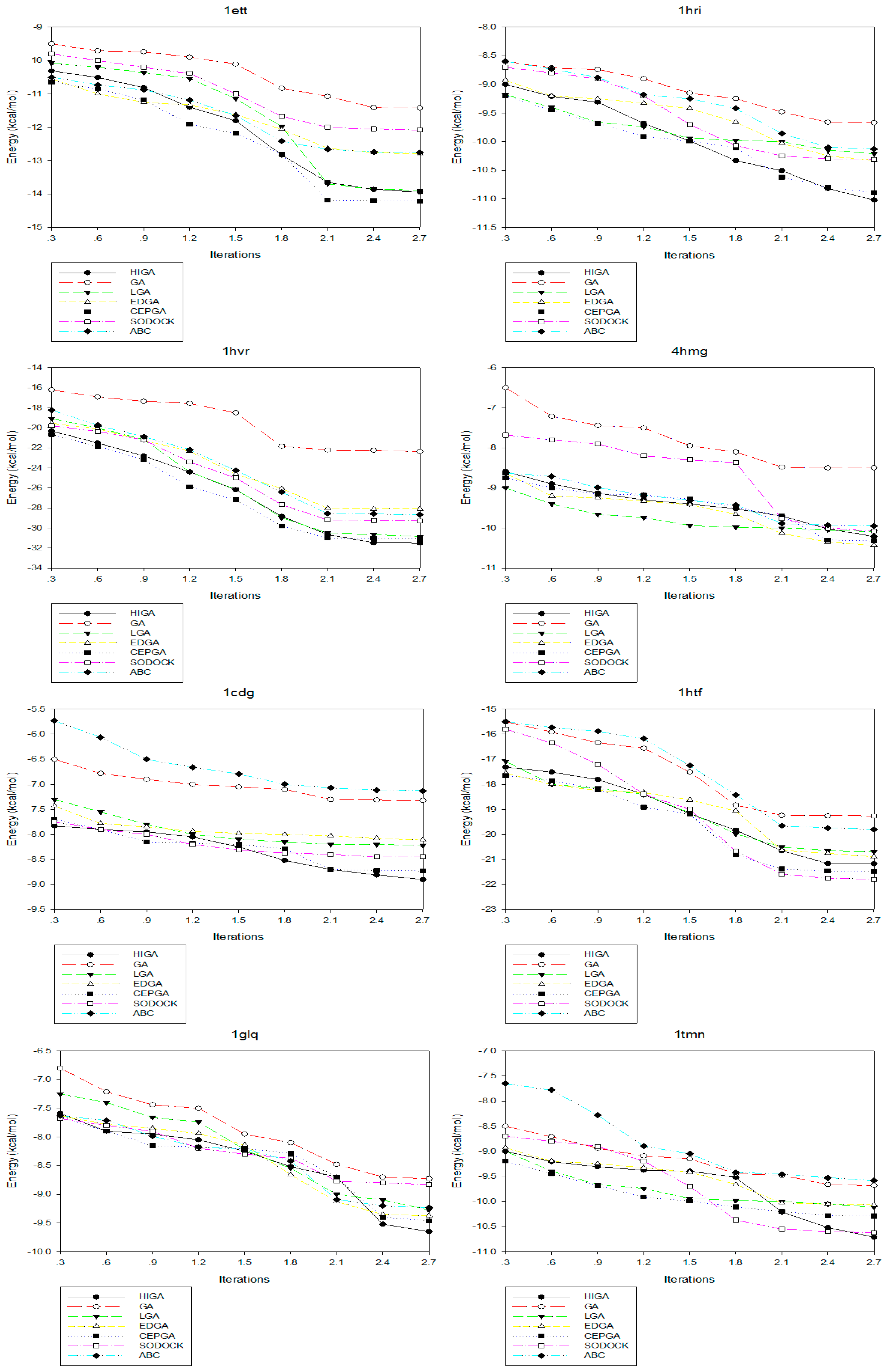
2.4. Convergence Analysis
Convergence means that the convergence curve of the objective solution tends to be stable after several iterations. The convergence diagrams of seven different algorithms for solving different test cases of Dataset 2 are shown in Figure 2. The number of iterations is 3000, 6000, 9000, 12,000, 15,000, 18,000, 21,000, 24,000 and 27,000, respectively, and these values are used as the horizontal axis of the convergence diagrams. The energy of each algorithm under different iteration times is calculated as the vertical axis. At the early stage of each algorithm, the energy value decreases as the number of iterations increases. But, in the later stage, the energy values of some algorithms tend to be fixed. This phenomenon, which is caused by the decrease of population diversity and the loss of evolutionary capacity, is called premature convergence. For example, LGA, EDGA, and SODOCK are prematurely convergent after iterating 15,000 times in 2mcp; GA and ABC are prematurely convergent after iterating 18,000 times in 2mcp; LGA, EDGA, SODOCK, and ABC are prematurely convergent after iterating 21,000 times in 6rnt. From these graphs, it can be concluded that HIGA is superior to other algorithms regarding preventing premature and solution quality.
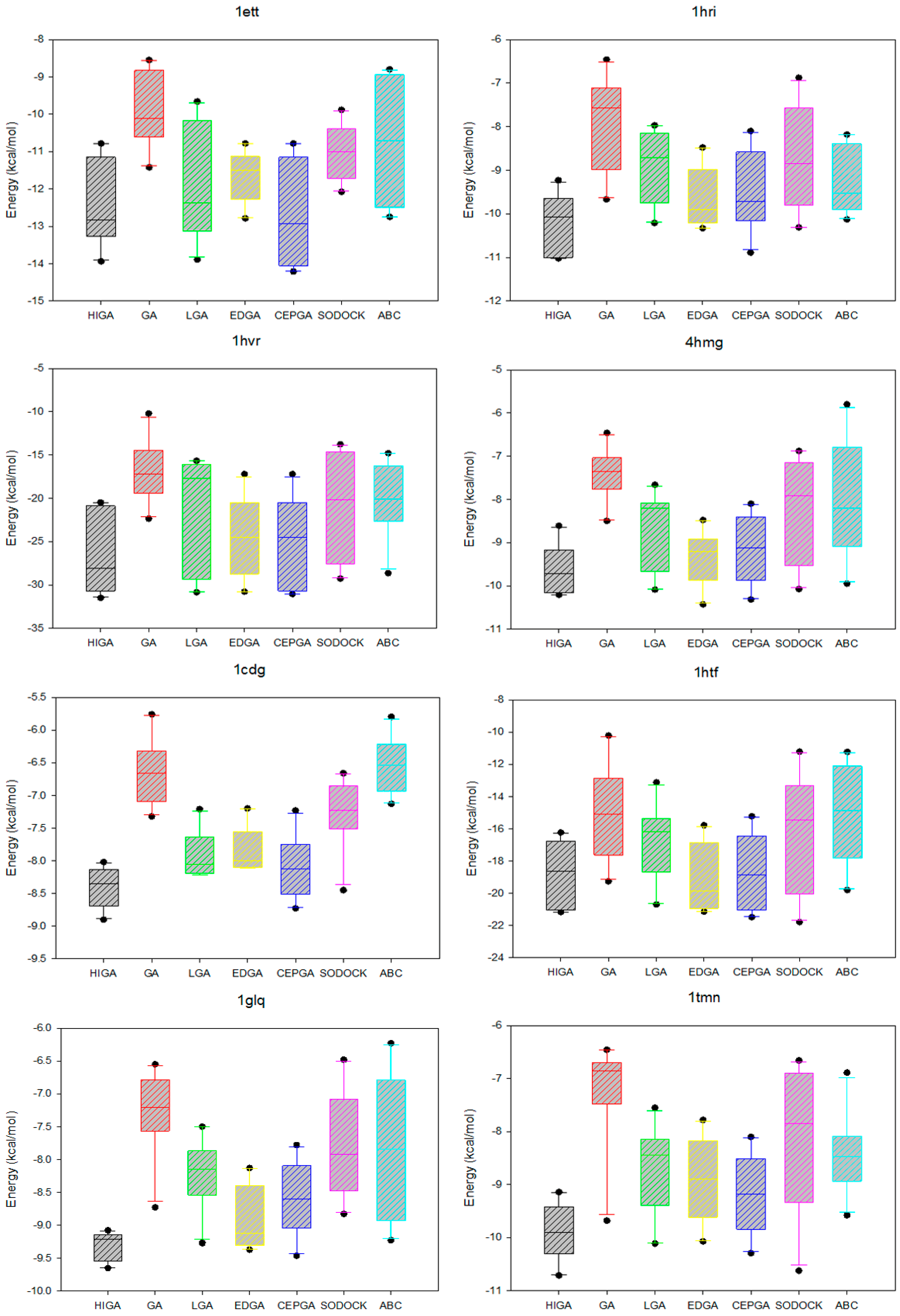
2.5. Data Distribution Analysis
The data distribution can reflect the concentration of the data and the stability of the algorithm. We calculate the minimum, the first quartile, the median, the third quartile, and the maximum of the energy values of each PDB, and then we use the five statistical quantities to draw the box plots (Figure 3). The median, which is not affected by the extreme data, is suitable as a centralized trend value. It is evident that the median energy of HIGA is lower than that of the other algorithms. The first quartile is the upper boundary of the box, the third quartile is the lower boundary of the box, and the data distribution is concentrated or dispersed and can be determined by observing the box. It can be seen that the data distribution of HIGA is the most concentrated. The points outside the maximum and minimum are the outliers, and the outliers have an undesirable consequence of data distribution. For example, the outlier of GA in 1glq; the outlier of LGA in 3hvt; the outlier of EDGA in 1stp; the outlier of SODOCK in 1cdg; the outlier of ABC in 4hmg. HIGA and CEPGA have no outliers. It can be concluded that HIGA is a stable method for protein-ligand docking.
2.6. Execution Time Analysis
The execution time of the seven compared algorithms for solving different complexes of Dataset 2 are shown in Table 4. The time is recorded by how many seconds per run. There a direct relation between the execution time and the problem complexity. In addition to a few complexes, the execution time of the algorithms increases as the number of rotatable bonds increases. As seen from the table, the execution time of GA is the fastest, followed by LGA, EDGA, CEPGA, HIGA, ABC, and SODOCK. The best performance algorithm HIGA in previous experiments does not play an advantage in the time performance. However, the execution time of HIGA is not greatly increased when compared to the fastest algorithm GA. This can demonstrate that HIGA does not raise the performance at the cost of increasing the execution time.
2.7. Comparison Based on the Hypothesis Test
We use the hypothesis test to determine the difference between each algorithm in Table 5. Five of the best values obtained by each algorithm for every PDB are taken, and the critical value of hypothesis test is set to 0.05. When comparing algorithm A to algorithm B, we can conclude the algorithm A is significantly different from the algorithm B if the p-value is less than 0.05. The significant difference demonstrates that the algorithm A is superior to the algorithm B. As seen from the table, HIGA, EDGA, and CEPGA are better than GA, LGA, SODOCK, and ABC in most of the PDBs. Furthermore, HIGA is better than EDGA and CEPGA according to the p-value. We can make a conclusion from the statistical analysis that HIGA is significantly better than the other algorithms.
3. Materials and Methods
3.1. Running History Information Guided Genetic Algorithm
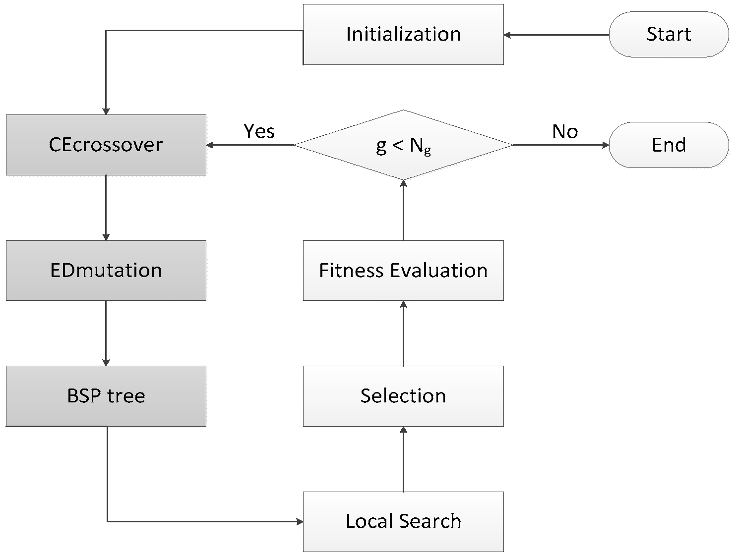
HIGA is an LGA-based hybrid search algorithm that is designed for protein-ligand docking. GA is an algorithm for simulating natural evolution process, and it generates solutions to optimise problems with the assistance of mutation, selection, and crossover. In each iteration of the genetic algorithm, the individual selection is made according to the fitness of the individual in the feasible region of the problem. Thus, a new and better approximate solution is generated. GA is simple, easy to realize, and has high robustness, so it has been successfully applied to solve the protein-ligand docking problem. LGA, which combines GA with local search method, searches the potential energy surface rapidly by GA and optimises the potential energy surface by local search method. LGA is proved to be an effective method for the protein-ligand docking, but the solutions that are obtained by LGA are unstable because of its randomness. Therefore, HIGA is proposed to overcome the drawback. Three core mechanisms are used to enhance the performance of HIGA for docking problems, and they are CE crossover, ED muation, and binary space partitioning (BSP) tree. CE crossover uses history information to improve the randomness of crossover operation. ED muation can guide the solutions to evolve in a better direction. BSP tree can memorize evaluated solutions that it has visited so that the diversity of solutions is maintained and the waste of computer resources is reduced. Taking the three techniques into consideration, the novel algorithm is guided to find some promising solutions by the running history information. Figure 4 is the block diagram of HIGA, and the grey parts are the three innovative mechanisms, which are newly added into LGA. HIGA first initializes the population randomly, and then obtains the next population by CE crossover, ED mutation, BSP tree, local search, selection and fitness evaluation. The process is iterated until a preset termination condition is reached.
3.2. CE Crossover
Since the parents of elite individuals are not preserved in the crossover process of LGA, the chances of getting better solutions are reduced by the subsequent crossover operation. CE crossover is proposed to solve the problem in this section. This new crossover can preserve the parents of the elite individuals with the best solution so that the good genes can be extended to improve the quality of the next-generation population. Table 6 shows the pseudocode of CE crossover. In the strategy, Mfather and Mmother are introduced, in which Mfather and Mmother represent the parents of the elite individual, e. The individual with current optimum fitness is selected as the elite individual at current iteration, and Mfather and Mmother are saved. The preserved individuals and the individuals of next-generation form a new population. The genes of these preserved individuals are excellent, and the possibility that they continue to reproduce individuals with good genes is greater. For each iteration, the number of elite individuals is set up to a certain percentage of the number of individuals, and the default is ten percent.
3.3. ED Mutation
In LGA, some genes of the individuals are random changes by mutation operation, which results in the search direction of the algorithm is also random and aimless. At the early stage of this algorithm, the randomness plays a very positive guiding effect for global search. It is because the optimal solution in which the direction is unknown in the case of no search experience. With the continuous iteration of the algorithm, the group search experience is accumulating, the direction is gradually clear, and the search space starts to converge gradually. This means that the current best solution is inevitably abandoned, even the global best solution. Therefore, ED mutation is proposed to optimize the search direction. The pseudocode of ED mutation is shown in Table 7. Where mi is the current solution; θ and are random numbers; β is a particular adjustable parameter, Moptimum is the historic optimal solution; and, Msub represents is the historic suboptimal solution; Mmax is the maximum solution; Mmin is the minimum solution. In the formula, the historic optimal solution and the historic suboptimal solution are used to ensure the correctness of the optimal solution direction. This mechanism is similar to the addition of vectors, and the addition can ensure that the algorithm evolves towards a better direction.
3.4. BSP Tree
The BSP tree that has been applied in non-revisiting genetic algorithm (NrGA) is used to store the evaluated solutions, and it divides the search space in accordance with the cumulative distribution of the solutions being evaluated. The BSP tree has only one root node at the beginning, and this node represents the entire search space. Each node that is subsequently inserted into BSP tree represents a subspace. If a parent node has two child nodes (l and r), the subspaces that are represented by the two child nodes are disjoint, and the sum of the two spaces is the subspace corresponding to the parent node. BSP tree is different from with Octree employed in QuickVina-W [41]. BSP tree stores all of the solutions that the algorithm has searched before, while Octree stores high-quality history points which are the output of last iteration of local optimization from all of the searching threads during the runtime. Table 8 shows the pseudo code for the working principle of BSP tree. Where RF is the revisit flag; and, d is the distance between two nodes. The position of each previous individual generated by the algorithm is recorded in a node of the tree. When the new generated individual m visits the node l or r, their positions are checked. If m = l or m = r, m is revisited and RF is 1. If the solution is revisited, it mutates to a nearest unvisited neighbor subspace. BSP tree can guarantee the location of all solutions is different so that the diversity of the individuals is maintained and the sample space of GA is increased.
4. Conclusions
The article presents HIGA, which combines binary space partitioning (BSP), ED muation, and CE crossover to extend the power of the LGA-based algorithm. CE crossover amplifies the probability of repeated use of the individual with good genes, so that HIGA is more suitable to the changes of the environment evolution. ED mutation provides a guarantee for the evolutionary direction of HIGA, and its concept originates from the property of vector addition. By using the BSP tree, the search algorithm can not only remove revisits, but also guide to search for the next unvisited position. We have compared the performance of HIGA, GA, LGA, EDGA, CEPGA, SODOCK, and ABC, the results of which indicate that HIGA outperforms that the other algorithms, suggesting that HIGA can enhance the power of AutoDock to protein-ligand docking.
Acknowledgments
This work was supported by the National Natural Science Foundation Program of China (61772124), the State Key Program of National Natural Science of China (61332014), the Fundamental Research Funds for the Central Universities under Grant 150402002 and Grant 150404008, and the Peak Discipline Construction of Computer Science and Technology under Grant 02190021821001.
Author Contributions
B.G. and Y.Z. conceived and designed the experiments; B.G. and C.Z. performed the experiments; B.G. and C.Z. analyzed the data; B.G. wrote the manuscript.
Conflicts of Interest
The authors declare no conflict of interest.
References
- Bohlooli, F.; Sepehri, S.; Razzaghi-AsI, N. Response surface methodology in drug design: A case study on docking analysis of a potent antifungal fluconazole. Comput. Biol. Chem. 2017, 67, 158–173. [Google Scholar] [CrossRef] [PubMed]
- Zhao, Y.H.; Wang, G.R.; Yin, Y. Improving ELM-based microarray data classification by diversified sequence features selection. Neural Comput. Appl. 2016, 27, 155–166. [Google Scholar] [CrossRef]
- Li, Y.; Zhao, Y.H.; Wang, G.R.; Wang, Z.H.; Gao, M. ELM-Based Large-Scale Genetic Association Study via Statistically Significant Pattern. IEEE Trans. Syst. Man Cybern. Syst. 2017, 1–14. [Google Scholar] [CrossRef]
- Allen, S.E.; Dokholyan, N.V.; Bowers, A.A. Dynamic docking of conformationally constrained macrocycles: Methods and applications. ACS Chem. Biol. 2016, 11, 10–24. [Google Scholar] [CrossRef] [PubMed]
- Zou, Q.; Li, J.J.; Song, L.; Zeng, X.X.; Wang, G.H. Similarity computation strategies in the microRNA-disease network: A Survey. Brief. Funct. Genom. 2016, 15, 55–64. [Google Scholar] [CrossRef] [PubMed]
- Bjerrum, E.J. Machine learning optimization of cross docking accuracy. Comput. Biol. Chem. 2016, 62, 133–144. [Google Scholar] [CrossRef] [PubMed]
- Guedes, I.A.; de Magalhães, C.S.; Dardenne, L.E. Receptor-ligand molecular docking. Biophys. Rev. 2014, 6, 75–87. [Google Scholar] [CrossRef] [PubMed]
- Huang, S.Y.; Zou, X.Q. Advances and challenges in protein-ligand docking. Int. J. Mol. Sci. 2010, 11, 3016–3034. [Google Scholar] [CrossRef] [PubMed]
- Jug, G.; Anderluh, M.; Tomašič, T. Comparative evaluation of several docking tools for docking small molecule ligands to DC-SIGN. J. Mol. Model. 2015, 21, 164–178. [Google Scholar] [CrossRef] [PubMed]
- Zhao, Y.H.; Wang, G.R.; Zhang, X.; Yu, J.X.; Wang, Z.H. Learning Phenotype Structure Using Sequence Model. IEEE Trans. Knowl. Data Eng. 2014, 26, 667–681. [Google Scholar] [CrossRef]
- Zhao, Y.H.; Yu, J.X.; Wang, G.R.; Chen, L.; Wang, B.; Yu, G. Maximal Subspace Coregulated Gene Clustering. IEEE Trans. Knowl. Data Eng. 2008, 20, 83–98. [Google Scholar] [CrossRef]
- Zeng, X.X.; Liao, Y.L.; Liu, Y.S.; Zou, Q. Prediction and validation of disease genes using HeteSim Scores. IEEE ACM Trans. Comput. Biol. Bioinform. 2017, 14, 687–695. [Google Scholar] [CrossRef] [PubMed]
- Moitessier, N.; Englebienne, P.; Lee, D.; Lawandi, J.; Gorbeil, C.R. Towards the development of universal, fast and highly accurate docking/scoring methods: A long way to go. Br. J. Pharmacol. 2008, 153, 7–26. [Google Scholar] [CrossRef] [PubMed]
- Hu, X.; Balaz, S.; Shelver, W.H. A practical approach to docking of zinc metalloproteinase inhibitors. J. Mol. Graph. Model. 2004, 22, 293–307. [Google Scholar] [CrossRef] [PubMed]
- Huey, R.; Morris, G.M.; Olson, A.J.; Goodsell, D.S. Software news and update a semiempirical free energy force field with charge-based desolvation. J. Comput. Chem. 2006, 10, 1145–1152. [Google Scholar]
- Jain, A.N. Scoring functions for protein-ligand docking. Curr. Protein Pept. Sci. 2006, 7, 407–420. [Google Scholar] [PubMed]
- Muryshev, A.E.; Tarasov, D.N.; Butygin, A.V.; Butygina, O.V.; Aleksandrov, A.B.; Nikitin, S.M. A novel scoring function for molecular docking. J. Comput. Aided Mol. Des. 2003, 17, 597–605. [Google Scholar] [CrossRef] [PubMed]
- Bharatham, N.; Bharatham, K.; Shelat, A.A.; Bashford, D. Ligand binding more prediction by docking: Mdm2/mdmx inhibitors as a case study. J. Chem. Inf. Model. 2014, 54, 648–659. [Google Scholar] [CrossRef] [PubMed]
- Li, Z.F.; Gu, J.F.; Zhuan, H.Y.; Kang, L.; Zhao, X.Y.; Guo, Q. Adaptive molecular docking method baesd on information entropy genetic algorithm. Appl. Soft Comput. 2015, 26, 299–302. [Google Scholar] [CrossRef]
- Feinstein, W.P.; Brylinski, M. Calculating an optimal box size for ligand docking and virtual screening against experimental and predicted binding pockets. J. Cheminform. 2015, 7. [Google Scholar] [CrossRef] [PubMed]
- Ain, Q.U.; Aleksandrova, A.; Roessler, F.D.; Ballester, P.J. Machine-learning scoring functions to improve structure-based binding affinity prediction and virtual screening. Wiley Interdiscip. Rev. Comput. Mol. Sci. 2015, 5, 405–424. [Google Scholar] [CrossRef] [PubMed]
- Guo, L.Y.; Yan, Z.Q.; Zheng, X.L.; Hu, L.; Yang, Y.L.; Wang, J. A comparison of various optimization algorithms of protein-ligand docking programs by fitness accuracy. J. Mol. Model. 2014, 20. [Google Scholar] [CrossRef] [PubMed]
- Blum, C.; Puchinger, J.; Raidl, G.R.; Roli, A. Hybrid mataheuristics in combinatorial optimization: A survey. Appl. Soft Comput. 2011, 11, 4135–4151. [Google Scholar] [CrossRef]
- Lόpez-Camacho, E.; Godoy, M.J.; Garcỉa-Nieto, J.; Nebro, A.J.; Aldana-Montes, J.F. Solving molecular flexible docking problems with mataheuristics: A comparative study. Appl. Soft Comput. 2015, 28, 379–393. [Google Scholar] [CrossRef]
- Goodsell, D.S.; Olson, A.J. Automated docking of substrates to proteins by simulated annealing. Proteins Struct. Funct. Genet. 1990, 8, 195–202. [Google Scholar] [CrossRef] [PubMed]
- Cao, T.C.; Li, T.H. A combination of numeric genetic algorithm and tabu search can be applied to molecular docking. Comput. Biol. Chem. 2004, 28, 303–312. [Google Scholar]
- Jones, G.; Willett, P.; Glen, R.C.; Leach, A.R.; Taylor, R. Development and validation of a genetic algorithm for flexible docking. J. Mol. Biol. 1997, 267, 727–748. [Google Scholar] [CrossRef] [PubMed]
- Thomsen, R. Flexible ligand docking using evolutionary algorithms: Investigating the effects of variation operators and local search hybrids. Biosystems 2003, 72, 57–73. [Google Scholar] [CrossRef]
- Fuhrmann, J.; Rurainsk, A.; Lenhof, H.P.; Neumann, D. A new Lamarckian genetic algorithm for flexible ligang-receptor docking. J. Comput. Chem. 2010, 31, 1911–1918. [Google Scholar] [PubMed]
- Chen, H.M.; Liu, B.F.; Huang, H.L.; Hwang, S.F.; Ho, S.Y. SODOCK: Swarm optimization for highly flexible protein-ligand docking. J. Comput. Chem. 2007, 28, 612–623. [Google Scholar] [CrossRef] [PubMed]
- Jason, S.; Merkle, D.; Middendorf, M. Molecular docking with multi-objective particle swarm optimization. Appl. Soft Comput. 2008, 8, 666–675. [Google Scholar] [CrossRef]
- Ng, M.C.; Fong, S.; Siu, S.W. PSOVina: The hybrid particle swarm optimization algorithm for protein-ligand docking. J. Bioinform. Comput. Biol. 2015, 13. [Google Scholar] [CrossRef] [PubMed]
- Uehara, S.; Fujimoto, K.J.; Tanaka, S. Protein-ligand docking using fitness learning-based artificial bee colony with proximity stimuli. Phys. Chem. Chem. Phys. 2015, 17, 16412–16417. [Google Scholar] [CrossRef] [PubMed]
- Guan, B.X.; Zhang, C.S.; Ning, J.X. Genetic Algorithm with a Crossover Elitist Preservation Mechanism for Protein-Ligand Docking. AMB Express 2017, 7. [Google Scholar] [CrossRef] [PubMed]
- Guan, B.X.; Zhang, C.S.; Ning, J.X. EDGA: A Population Evolution Direction Guided Genetic Algorithm for Protein-Ligand Docking. J. Comput. Biol. 2016, 23, 585–596. [Google Scholar] [CrossRef] [PubMed]
- Yuen, S.Y.; Chow, C.K. A genetic algorithm that adaptively mutates and never revisits. IEEE. Trans. Evol. Comput. 2009, 13, 454–472. [Google Scholar] [CrossRef]
- Kitchen, D.B.; Decomez, H.; Furr, J.R.; Bajorath, J. Docking and scoring in virtual screening for drug discovery: Methods and applications. Nat. Rev. Drug Discov. 2004, 3, 935–949. [Google Scholar] [CrossRef] [PubMed]
- Morris, G.M.; Huey, R.; Lindstrom, W.; Sanner, M.F.; Belew, R.K.; Goodsell, D.S.; Olson, A.J. AutoDock4 and AutoDockTools4: Automated docking with selective receptor flexibility. J. Comput. Chem. 2009, 30, 2785–2791. [Google Scholar] [CrossRef] [PubMed]
- Castro-Alvarez, A.; Costa, A.M.; Vilarrasa, J. The Performance of Several Docking Programs at Reproducing Protein-Macrolide-Like Crystal Structures. Molecules 2017, 22, 136. [Google Scholar] [CrossRef] [PubMed]
- Wang, R.X.; Fang, X.L.; Lu, Y.P.; Yang, C.Y.; Wang, S.M. The PDBbind database: Methodologies and updates. J. Med. Chem. 2005, 48, 4111–4119. [Google Scholar] [CrossRef] [PubMed]
- Hassan, N.M.; Alhossary, A.A.; Mu, Y.G.; Kwoh, C.K. Protein-Ligand Blind Docking Using QuickVina-W with Inter-Process Spatio-Temporal Integration. Sci. Rep. 2017, 7. [Google Scholar] [CrossRef] [PubMed]
Sample Availability: Not available. |
Figure 1.
The molecular structures of ligands.
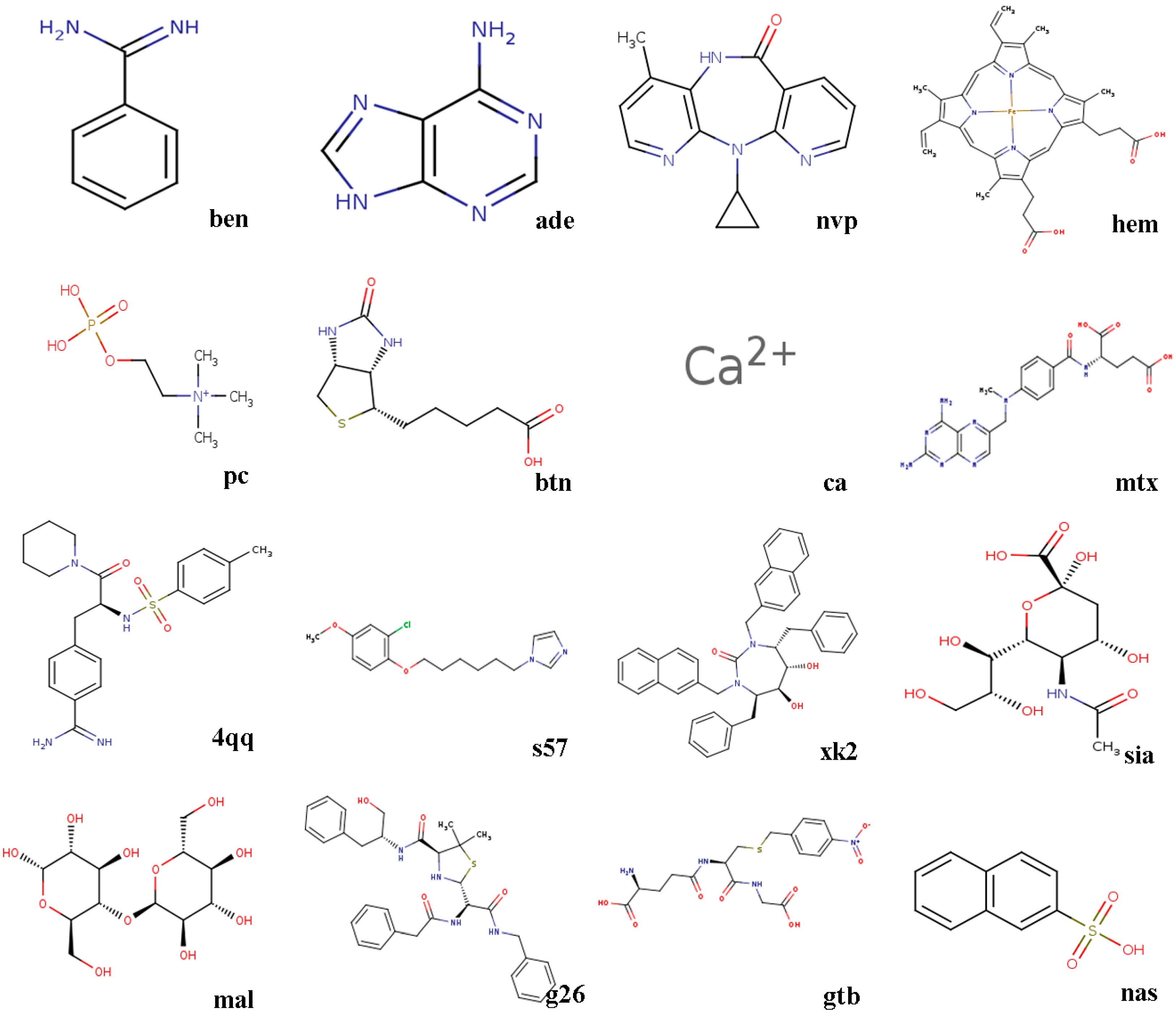
Figure 2.
Convergence diagrams of seven algorithms in different X-ray crystallographic complexes (PDB).
Figure 2.
Convergence diagrams of seven algorithms in different X-ray crystallographic complexes (PDB).
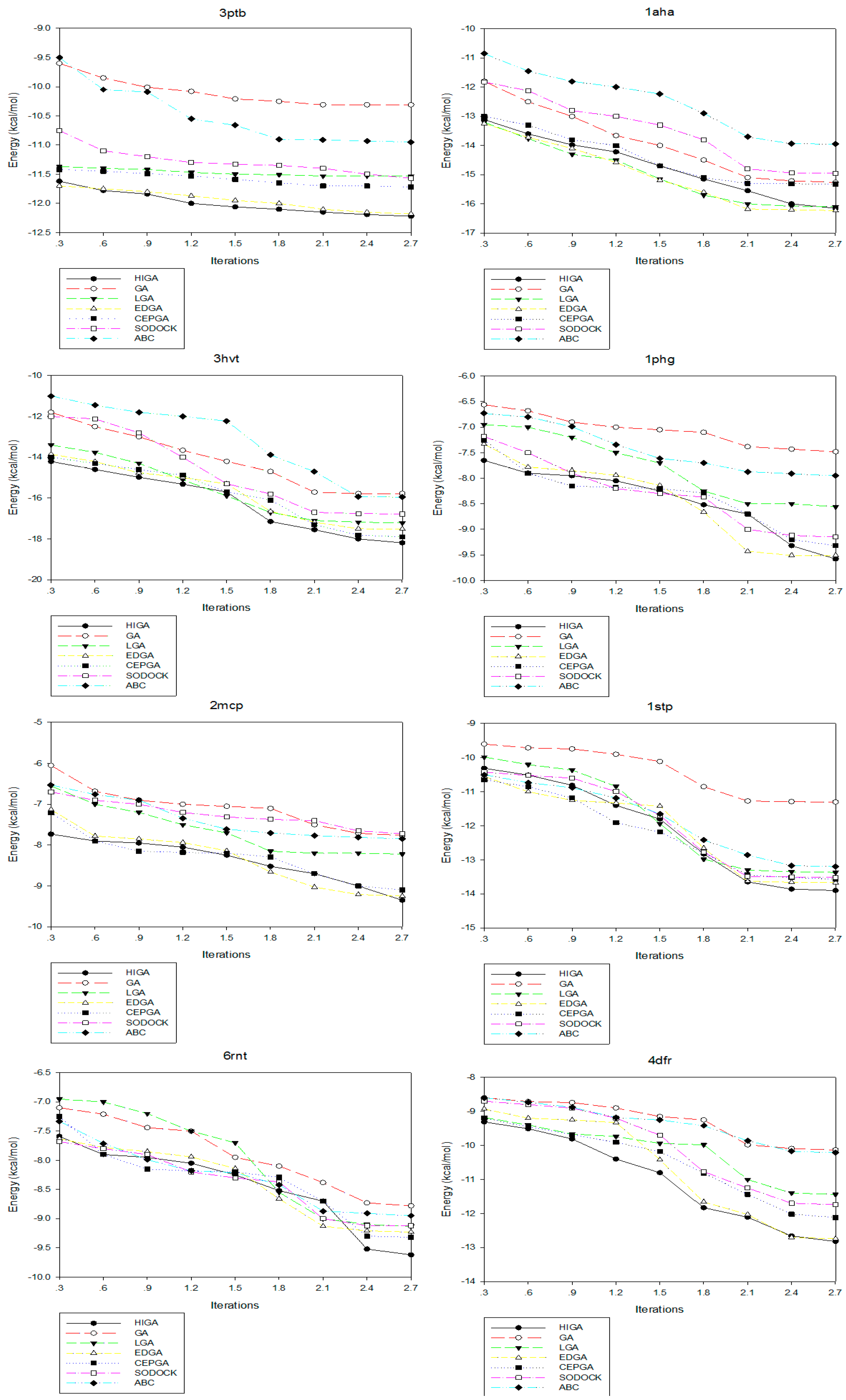

Figure 3.
Box plots of seven algorithms in different PDB.
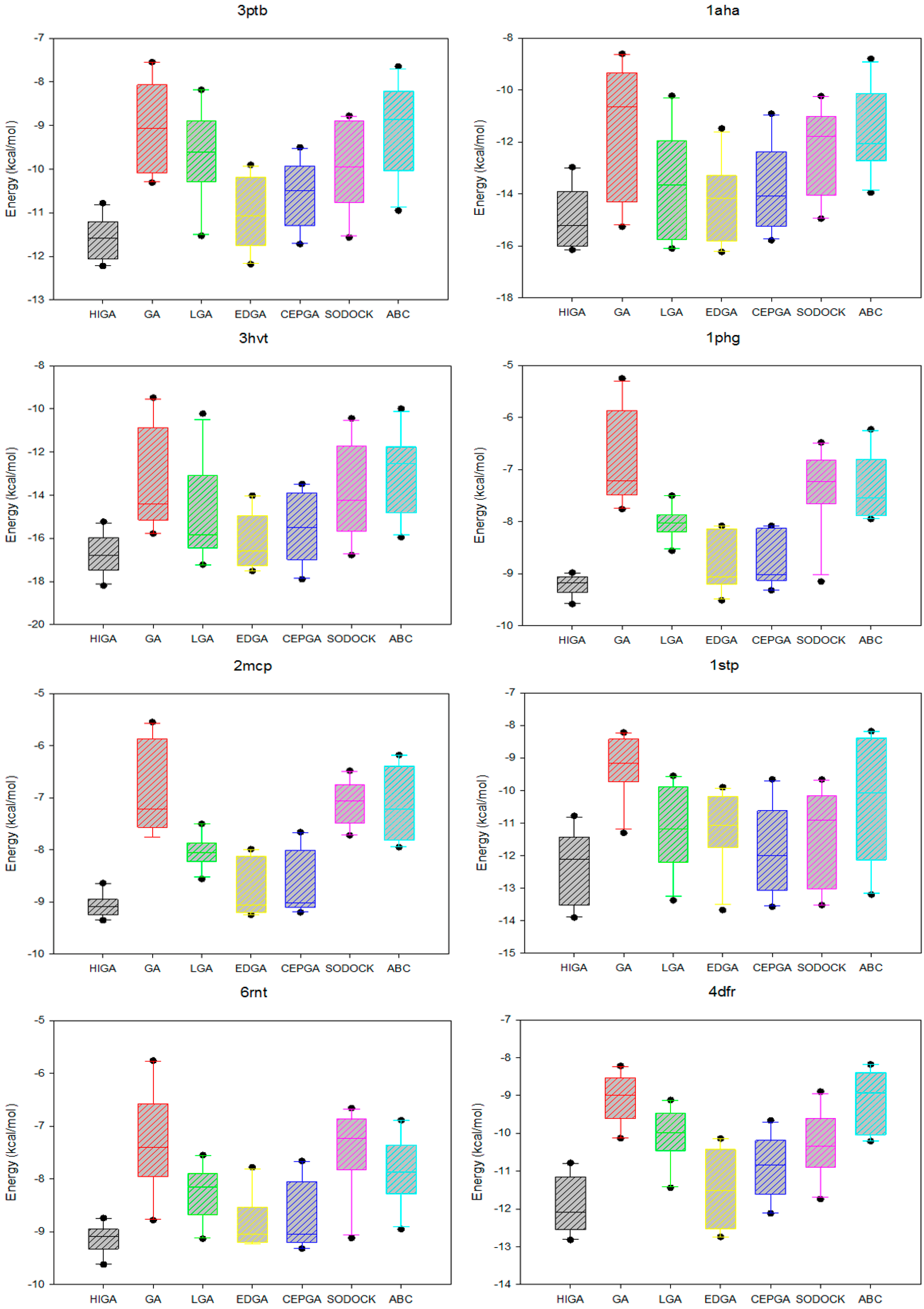

Figure 4.
Block diagram of HIGA.

Table 1.
Results of success case and average root-mean-square positional deviation (RMSD).
| Algorithm | Success Case | Average RMSD (All Cases) | Average RMSD (RMSD < 2 Å) |
|---|---|---|---|
| HIGA | 90 | 1.81 | 1.32 |
| GA | 58 | 3.12 | 1.80 |
| LGA | 68 | 2.55 | 1.69 |
| EDGA | 77 | 2.21 | 1.62 |
| CEPGA | 81 | 2.13 | 1.59 |
| SODOCK | 73 | 2.88 | 1.79 |
| ABC | 62 | 3.25 | 1.83 |
Table 2.
The lowest energy and RMSD results.
| HIGA | GA | LGA | EDGA | CEPGA | SODOCK | ABC | ||||||||||
|---|---|---|---|---|---|---|---|---|---|---|---|---|---|---|---|---|
| PDB | Ligand | Torsions | Energy | RMSD | Energy | RMSD | Energy | RMSD | Energy | RMSD | Energy | RMSD | Energy | RMSD | Energy | RMSD |
| 3ptb | ben | 0 | −12.22 | 1.95 | −10.31 | 1.66 | −11.53 | 1.92 | −12.18 | 1.95 | −11.72 | 1.90 | −11.57 | 2.00 | −10.95 | 1.97 |
| 1aha | ade | 1 | −16.15 | 0.90 | −15.26 | 1.20 | −16.10 | 0.45 | −16.23 | 0.38 | −15.32 | 0.89 | −14.95 | 1.44 | −13.95 | 1.85 |
| 3hvt | nvp | 2 | −18.19 | 0.45 | −15.78 | 0.40 | −17.22 | 0.33 | −17.52 | 0.53 | −17.90 | 0.30 | −16.78 | 0.58 | −15.95 | 0.68 |
| 1phg | hem | 3 | −9.58 | 0.60 | −7.48 | 1.25 | −8.56 | 0.80 | −9.51 | 0.70 | −9.32 | 0.64 | −9.15 | 1.34 | −7.95 | 1.67 |
| 2mcp | pc | 4 | −9.35 | 1.15 | −7.76 | 1.46 | −8.22 | 1.33 | −9.25 | 1.23 | −9.10 | 1.20 | −7.72 | 1.42 | −7.85 | 1.64 |
| 1stp | btn | 5 | −13.90 | 0.85 | −11.30 | 1.84 | −13.37 | 1.65 | −13.67 | 1.25 | −13.57 | 0.90 | −13.52 | 1.00 | −13.20 | 1.58 |
| 6rnt | ca | 6 | −9.62 | 0.50 | −8.78 | 0.65 | −9.13 | 0.70 | −9.23 | 0.85 | −9.32 | 0.58 | −9.12 | 1.95 | −8.95 | 1.45 |
| 4dfr | mtx | 7 | −12.82 | 1.56 | −10.13 | 0.90 | −11.44 | 1.23 | −12.74 | 1.59 | −12.12 | 1.90 | −11.74 | 1.67 | −10.21 | 1.97 |
| 1ett | 4qq | 8 | −13.94 | 1.40 | −11.42 | 1.62 | −13.89 | 1.38 | −12.79 | 1.20 | −14.21 | 1.29 | −12.08 | 1.54 | −12.75 | 1.65 |
| 1hri | s57 | 9 | −11.02 | 1.18 | −9.67 | 1.80 | −10.21 | 1.87 | −10.33 | 1.37 | −10.89 | 1.38 | −10.31 | 1.68 | −10.13 | 1.67 |
| 1hvr | xk2 | 10 | −31.50 | 0.80 | −22.35 | 1.08 | −30.85 | 0.62 | −28.10 | 0.75 | −31.06 | 0.64 | −29.29 | 0.68 | −28.65 | 0.85 |
| 4hmg | sia | 11 | −10.21 | 1.65 | −8.50 | 1.68 | −10.09 | 1.70 | −10.43 | 1.58 | −10.32 | 1.89 | −10.08 | 1.36 | −9.95 | 1.60 |
| 1cdg | mal | 12 | −8.90 | 1.65 | −7.32 | 1.69 | −8.22 | 1.94 | −8.11 | 1.54 | −8.73 | 1.48 | −8.45 | 1.80 | −7.13 | 1.12 |
| 1htf | g26 | 13 | −21.17 | 1.20 | −19.26 | 1.58 | −20.69 | 1.33 | −20.89 | 1.30 | −21.48 | 1.27 | −21.79 | 1.42 | −19.80 | 1.80 |
| 1glq | gtb | 14 | −9.65 | 1.25 | −8.73 | 1.27 | −9.27 | 1.87 | −9.37 | 1.60 | −9.46 | 1.38 | −8.83 | 1.90 | −9.23 | 1.58 |
| 1tmn | nas | 15 | −10.71 | 0.95 | −9.68 | 1.11 | −10.11 | 1.20 | −10.07 | 1.45 | −10.29 | 0.85 | −10.62 | 1.95 | −9.58 | 0.65 |
Table 3.
Results of the rate of clusters and the rate in rank 1.
| Algorithm | HIGA | GA | LGA | EDGA | CEPGA | SODOCK | ABC |
|---|---|---|---|---|---|---|---|
| Number of clusters | 3.72 | 14.00 | 4.58 | 4.24 | 4.04 | 10.30 | 13.04 |
| Number in rank 1 | 17.04 | 8.00 | 15.72 | 15.92 | 16.20 | 11.82 | 8.70 |
Table 4.
Results of execution time.
| PDB | Torsions | HIGA | GA | LGA | EDGA | CEPGA | SODOCK | ABC |
|---|---|---|---|---|---|---|---|---|
| 3ptb | 0 | 1.79 | 1.56 | 1.74 | 1.77 | 1.75 | 1.89 | 1.90 |
| 1aha | 1 | 1.91 | 1.62 | 1.80 | 1.83 | 1.90 | 1.95 | 2.08 |
| 3hvt | 2 | 1.97 | 1.75 | 1.93 | 1.95 | 1.96 | 1.94 | 2.13 |
| 1phg | 3 | 2.75 | 2.21 | 2.55 | 2.61 | 2.70 | 2.23 | 2.65 |
| 2mcp | 4 | 2.72 | 2.35 | 2.62 | 2.70 | 2.68 | 2.51 | 2.69 |
| 1stp | 5 | 3.79 | 3.01 | 3.53 | 3.77 | 3.59 | 3.84 | 3.81 |
| 6rnt | 6 | 3.84 | 3.12 | 3.14 | 3.70 | 3.54 | 4.27 | 3.64 |
| 4dfr | 7 | 5.47 | 4.98 | 5.18 | 5.33 | 5.45 | 4.99 | 6.06 |
| 1ett | 8 | 8.44 | 7.83 | 8.17 | 8.28 | 8.37 | 8.29 | 7.97 |
| 1hri | 9 | 10.49 | 10.15 | 10.37 | 10.39 | 10.41 | 12.34 | 11.06 |
| 1hvr | 10 | 12.53 | 12.07 | 12.13 | 12.28 | 12.51 | 14.86 | 11.92 |
| 4hmg | 11 | 13.90 | 13.21 | 13.84 | 13.95 | 13.89 | 16.09 | 13.60 |
| 1cdg | 12 | 12.71 | 12.38 | 12.59 | 12.61 | 12.66 | 15.92 | 13.06 |
| 1htf | 13 | 13.01 | 12.49 | 12.78 | 12.99 | 12.84 | 16.26 | 13.18 |
| 1glq | 14 | 15.87 | 14.95 | 15.50 | 15.77 | 15.85 | 20.12 | 17.22 |
| Average | 7.41 | 6.91 | 7.19 | 7.33 | 7.34 | 8.5 | 7.53 |
Table 5.
Results of hypothesis test.
| PDB | HIGA | GA | LGA | EDGA | CEPGA | SODOCK | ABC | |
|---|---|---|---|---|---|---|---|---|
| 3ptb | HIGA | - | 0.004 | 0.010 | 0.044 | 0.035 | 0.012 | 0.008 |
| GA | 0.996 | - | 0.992 | 0.995 | 0.994 | 0.993 | 0.688 | |
| LGA | 0.990 | 0.008 | - | 0.986 | 0.982 | 0.563 | 0.425 | |
| EDGA | 0.956 | 0.005 | 0.014 | - | 0.340 | 0.017 | 0.010 | |
| CEPGA | 0.965 | 0.006 | 0.018 | 0.660 | - | 0.028 | 0.011 | |
| SODOCK | 0.988 | 0.007 | 0.437 | 0.983 | 0.972 | - | 0.306 | |
| ABC | 0.992 | 0.312 | 0.575 | 0.990 | 0.989 | 0.694 | - | |
| 1aha | HIGA | - | 0.029 | 0.062 | 0.524 | 0.044 | 0.024 | 0.017 |
| GA | 0.971 | - | 0.964 | 0.988 | 0.905 | 0.342 | 0.260 | |
| LGA | 0.938 | 0.036 | - | 0.981 | 0.460 | 0.030 | 0.024 | |
| EDGA | 0.476 | 0.012 | 0.019 | - | 0.017 | 0.010 | 0.005 | |
| CEPGA | 0.956 | 0.095 | 0.540 | 0.983 | - | 0.038 | 0.027 | |
| SODOCK | 0.976 | 0.658 | 0.970 | 0.990 | 0.962 | - | 0.470 | |
| ABC | 0.983 | 0.740 | 0.976 | 0.995 | 0.973 | 0.530 | - | |
| 3hvt | HIGA | - | 0.005 | 0.017 | 0.020 | 0.023 | 0.012 | 0.008 |
| GA | 0.995 | - | 0.795 | 0.974 | 0.993 | 0.788 | 0.537 | |
| LGA | 0.983 | 0.205 | - | 0.878 | 0.965 | 0.324 | 0.208 | |
| EDGA | 0.980 | 0.026 | 0.122 | - | 0.515 | 0.103 | 0.033 | |
| CEPGA | 0.977 | 0.007 | 0.035 | 0.485 | - | 0.029 | 0.011 | |
| SODOCK | 0.988 | 0.212 | 0.676 | 0.897 | 0.971 | - | 0.215 | |
| ABC | 0.992 | 0.463 | 0.792 | 0.967 | 0.989 | 0.785 | - | |
| 1phg | HIGA | - | 0.006 | 0.015 | 0.242 | 0.046 | 0.023 | 0.010 |
| GA | 0.994 | - | 0.682 | 0.991 | 0.983 | 0.968 | 0.545 | |
| LGA | 0.985 | 0.318 | - | 0.976 | 0.962 | 0.620 | 0.422 | |
| EDGA | 0.758 | 0.009 | 0.024 | - | 0.440 | 0.038 | 0.015 | |
| CEPGA | 0.954 | 0.017 | 0.038 | 0.560 | - | 0.045 | 0.028 | |
| SODOCK | 0.977 | 0.032 | 0.380 | 0.962 | 0.955 | - | 0.240 | |
| ABC | 0.990 | 0.455 | 0.578 | 0.985 | 0.972 | 0.760 | - | |
| 2mcp | HIGA | - | 0.002 | 0.008 | 0.036 | 0.015 | 0.001 | 0.004 |
| GA | 0.998 | - | 0.792 | 0.994 | 0.992 | 0.492 | 0.610 | |
| LGA | 0.992 | 0.208 | - | 0.988 | 0.987 | 0.092 | 0.224 | |
| EDGA | 0.964 | 0.006 | 0.012 | - | 0.442 | 0.005 | 0.011 | |
| CEPGA | 0.985 | 0.008 | 0.013 | 0.558 | - | 0.007 | 0.012 | |
| SODOCK | 0.999 | 0.508 | 0.908 | 0.995 | 0.993 | - | 0.640 | |
| ABC | 0.996 | 0.390 | 0.776 | 0.989 | 0.988 | 0.360 | - | |
| 1stp | HIGA | - | 0.001 | 0.006 | 0.048 | 0.033 | 0.014 | 0.003 |
| GA | 0.999 | - | 0.791 | 0.964 | 0.952 | 0.892 | 0.587 | |
| LGA | 0.994 | 0.209 | - | 0.942 | 0.887 | 0.624 | 0.450 | |
| EDGA | 0.952 | 0.036 | 0.058 | - | 0.414 | 0.082 | 0.043 | |
| CEPGA | 0.967 | 0.048 | 0.113 | 0.586 | - | 0.208 | 0.062 | |
| SODOCK | 0.986 | 0.108 | 0.376 | 0.918 | 0.792 | - | 0.215 | |
| ABC | 0.997 | 0.413 | 0.550 | 0.957 | 0.938 | 0.785 | - | |
| 6rnt | HIGA | - | 0.005 | 0.020 | 0.022 | 0.038 | 0.015 | 0.007 |
| GA | 0.995 | - | 0.942 | 0.965 | 0.985 | 0.695 | 0.588 | |
| LGA | 0.980 | 0.058 | - | 0.792 | 0.888 | 0.368 | 0.127 | |
| EDGA | 0.978 | 0.035 | 0.208 | - | 0.504 | 0.059 | 0.040 | |
| CEPGA | 0.962 | 0.015 | 0.112 | 0.496 | - | 0.047 | 0.025 | |
| SODOCK | 0.985 | 0.305 | 0.632 | 0.941 | 0.953 | - | 0.404 | |
| ABC | 0.993 | 0.412 | 0.873 | 0.960 | 0.975 | 0.596 | - | |
| 4dfr | HIGA | - | 0.002 | 0.006 | 0.035 | 0.032 | 0.021 | 0.003 |
| GA | 0.998 | - | 0.961 | 0.993 | 0.985 | 0.972 | 0.587 | |
| LGA | 0.994 | 0.039 | - | 0.966 | 0.950 | 0.624 | 0.450 | |
| EDGA | 0.965 | 0.007 | 0.034 | - | 0.490 | 0.042 | 0.013 | |
| CEPGA | 0.968 | 0.015 | 0.050 | 0.510 | - | 0.060 | 0.016 | |
| SODOCK | 0.979 | 0.028 | 0.376 | 0.958 | 0.940 | - | 0.215 | |
| ABC | 0.997 | 0.413 | 0.550 | 0.987 | 0.984 | 0.785 | - | |
| 1ett | HIGA | - | 0.008 | 0.082 | 0.060 | 0.515 | 0.044 | 0.057 |
| GA | 0.992 | - | 0.986 | 0.925 | 0.998 | 0.562 | 0.637 | |
| LGA | 0.918 | 0.014 | - | 0.482 | 0.932 | 0.073 | 0.151 | |
| EDGA | 0.940 | 0.075 | 0.518 | - | 0.950 | 0.077 | 0.205 | |
| CEPGA | 0.485 | 0.002 | 0.068 | 0.050 | - | 0.040 | 0.045 | |
| SODOCK | 0.956 | 0.432 | 0.927 | 0.923 | 0.960 | - | 0.520 | |
| ABC | 0.943 | 0.363 | 0.849 | 0.795 | 0.955 | 0.480 | - | |
| 1hri | HIGA | - | 0.001 | 0.018 | 0.025 | 0.041 | 0.021 | 0.004 |
| GA | 0.999 | - | 0.976 | 0.997 | 0.998 | 0.982 | 0.635 | |
| LGA | 0.982 | 0.024 | - | 0.862 | 0.890 | 0.723 | 0.117 | |
| EDGA | 0.975 | 0.003 | 0.138 | - | 0.504 | 0.140 | 0.015 | |
| CEPGA | 0.959 | 0.002 | 0.110 | 0.406 | - | 0.130 | 0.010 | |
| SODOCK | 0.979 | 0.018 | 0.277 | 0.860 | 0.870 | - | 0.020 | |
| ABC | 0.996 | 0.365 | 0.883 | 0.985 | 0.990 | 0.980 | - | |
| 1hvr | HIGA | - | 0.002 | 0.030 | 0.012 | 0.045 | 0.021 | 0.014 |
| GA | 0.998 | - | 0.995 | 0.562 | 0.996 | 0.942 | 0.665 | |
| LGA | 0.970 | 0.005 | - | 0.026 | 0.957 | 0.177 | 0.044 | |
| EDGA | 0.988 | 0.438 | 0.974 | - | 0.982 | 0.711 | 0.609 | |
| CEPGA | 0.955 | 0.004 | 0.043 | 0.018 | - | 0.035 | 0.024 | |
| SODOCK | 0.979 | 0.058 | 0.823 | 0.289 | 0.965 | - | 0.368 | |
| ABC | 0.986 | 0.335 | 0.956 | 0.391 | 0.976 | 0.632 | - | |
| 4hmg | HIGA | - | 0.022 | 0.072 | 0.522 | 0.514 | 0.054 | 0.032 |
| GA | 0.978 | - | 0.972 | 0.995 | 0.985 | 0.928 | 0.900 | |
| LGA | 0.928 | 0.028 | - | 0.980 | 0.945 | 0.417 | 0.214 | |
| EDGA | 0.478 | 0.005 | 0.020 | - | 0.487 | 0.017 | 0.010 | |
| CEPGA | 0.486 | 0.015 | 0.045 | 0.513 | - | 0.042 | 0.026 | |
| SODOCK | 0.946 | 0.072 | 0.583 | 0.983 | 0.958 | - | 0.240 | |
| ABC | 0.968 | 0.100 | 0.786 | 0.990 | 0.974 | 0.760 | - | |
| 1cdg | HIGA | - | 0.003 | 0.021 | 0.014 | 0.037 | 0.032 | 0.001 |
| GA | 0.997 | - | 0.883 | 0.784 | 0.995 | 0.985 | 0.408 | |
| LGA | 0.979 | 0.117 | - | 0.483 | 0.952 | 0.763 | 0.105 | |
| EDGA | 0.986 | 0.216 | 0.517 | - | 0.983 | 0.844 | 0.125 | |
| CEPGA | 0.963 | 0.005 | 0.048 | 0.017 | - | 0.059 | 0.003 | |
| SODOCK | 0.968 | 0.015 | 0.237 | 0.156 | 0.941 | - | 0.012 | |
| ABC | 0.999 | 0.592 | 0.895 | 0.875 | 0.997 | 0.988 | - | |
| 1htf | HIGA | - | 0.015 | 0.243 | 0.480 | 0.544 | 0.624 | 0.030 |
| GA | 0.985 | - | 0.973 | 0.974 | 0.985 | 0.987 | 0.637 | |
| LGA | 0.753 | 0.027 | - | 0.652 | 0.759 | 0.883 | 0.251 | |
| EDGA | 0.520 | 0.016 | 0.348 | - | 0.618 | 0.640 | 0.235 | |
| CEPGA | 0.456 | 0.015 | 0.241 | 0.382 | - | 0.538 | 0.028 | |
| SODOCK | 0.376 | 0.013 | 0.127 | 0.360 | 0.462 | - | 0.017 | |
| ABC | 0.970 | 0.363 | 0.749 | 0.765 | 0.972 | 0.983 | - | |
| 1glq | HIGA | - | 0.001 | 0.012 | 0.018 | 0.022 | 0.002 | 0.005 |
| GA | 0.999 | - | 0.982 | 0.991 | 0.995 | 0.695 | 0.788 | |
| LGA | 0.988 | 0.018 | - | 0.955 | 0.965 | 0.163 | 0.227 | |
| EDGA | 0.982 | 0.009 | 0.045 | - | 0.510 | 0.039 | 0.042 | |
| CEPGA | 0.978 | 0.005 | 0.035 | 0.490 | - | 0.027 | 0.031 | |
| SODOCK | 0.998 | 0.305 | 0.837 | 0.961 | 0.973 | - | 0.704 | |
| ABC | 0.995 | 0.212 | 0.773 | 0.958 | 0.969 | 0.296 | - | |
| 1tmn | HIGA | - | 0.004 | 0.023 | 0.012 | 0.028 | 0.043 | 0.002 |
| GA | 0.996 | - | 0.783 | 0.692 | 0.965 | 0.983 | 0.408 | |
| LGA | 0.977 | 0.217 | - | 0.283 | 0.716 | 0.746 | 0.105 | |
| EDGA | 0.988 | 0.308 | 0.717 | - | 0.810 | 0.975 | 0.125 | |
| CEPGA | 0.972 | 0.035 | 0.284 | 0.190 | - | 0.644 | 0.028 | |
| SODOCK | 0.953 | 0.017 | 0.256 | 0.025 | 0.356 | - | 0.012 | |
| ABC | 0.998 | 0.592 | 0.895 | 0.875 | 0.972 | 0.988 | - |
Table 6.
Pseudocode of CE crossover.
| Algorithm: CE Crossover |
|---|
| Input: (1) a population with n indiviudals, (2) elitists e. |
| Output: a population after CE crossover |
| 01. For i: = 1 to n do |
| 02. Find the historial optimal individual m0 |
| 03. If the fitness of current individual mi < m0 then |
| 04. m0 = mi |
| 05. e = m0 |
| 06. preserve Mfather and Mmother |
| 07. End if |
| 08. Mfather, Mmother and e next population |
| 09. End for |
Table 7.
Pseudocode of ED mutation.
| Algorithm: ED Mutation |
|---|
| Input: (1) a population with n indiviudals, (2) balance factor β. |
| Output: a population after ED mutation |
| 01. For i: = 1 to n do |
| 02. Find the optimal solution Moptimum and the historic suboptimal solution Msub |
| 03. If θ < β then |
| 04. mi = mmin + θ (Mmax − Mmin) |
| 05. Else |
| 06. mi = mi + θ (Moptimum − Msub) +(Moptimum − mi) |
| 07. End if |
| 08. End for |
Table 8.
Pseudocode of BSP tree.
| Algorithm: BSP Tree |
|---|
| Input: (1) an individual m, (2) BSP tree T (3) revisit flag RF |
| Output: an individual m that never revisits |
| 01. Curr_node: = root node of T |
| 02. RF = 0 |
| 03. If (Curr_node has two child nodes: l and r) then |
| 04. Compare m with child node l and r |
| 05. If (m = l) or (m = r) then |
| 06. RF = 1 |
| 07. End if |
| 08. If d (l, m) < d (r, m) then |
| 09. Curr_node: = child node l |
| 10. Else |
| 11. Curr_node: = child node r |
| 12. End if |
| 13. Repeat steps 03-12 |
| 14. Else |
| 15. If (RF = 0) then |
| 16. Insert a child node to Curr_node that records m |
| 17. Else |
| 18. Creat a new child node by mutating |
| 19. End if |
| 20. End if |
© 2017 by the authors. Licensee MDPI, Basel, Switzerland. This article is an open access article distributed under the terms and conditions of the Creative Commons Attribution (CC BY) license (http://creativecommons.org/licenses/by/4.0/).
Share and Cite
MDPI and ACS Style
Guan, B.; Zhang, C.; Zhao, Y. HIGA: A Running History Information Guided Genetic Algorithm for Protein–Ligand Docking. Molecules 2017, 22, 2233. https://doi.org/10.3390/molecules22122233
AMA Style
Guan B, Zhang C, Zhao Y. HIGA: A Running History Information Guided Genetic Algorithm for Protein–Ligand Docking. Molecules. 2017; 22(12):2233. https://doi.org/10.3390/molecules22122233
Chicago/Turabian StyleGuan, Boxin, Changsheng Zhang, and Yuhai Zhao. 2017. "HIGA: A Running History Information Guided Genetic Algorithm for Protein–Ligand Docking" Molecules 22, no. 12: 2233. https://doi.org/10.3390/molecules22122233