Article

Molecular Insights into the Genetic Diversity of Hemarthria compressa Germplasm Collections Native to Southwest China

1
Department of Grassland Science, Animal Science and Technology College, Sichuan Agricultural University, Ya'an 625014, China
2
Sichuan Academy of Grassland Science, Chengdu 611731, China
3
Chongqing Municipal Institute of Animal Husbandry, Chongqing 400039, China
*
Author to whom correspondence should be addressed.
Molecules 2014, 19(12), 21541-21559; https://doi.org/10.3390/molecules191221541
Submission received: 16 October 2014 / Revised: 16 December 2014 / Accepted: 18 December 2014 / Published: 22 December 2014
(This article belongs to the Section Molecular Diversity)

Abstract

:
Start codon targeted polymorphism (SCoT) analysis was employed to distinguish 37 whipgrass (Hemarthria compressa L.) clones and assess the genetic diversity and population structure among these genotypes. The informativeness of markers was also estimated using various parameters. Using 25 highly reproducible primer sets, 368 discernible fragments were generated. Of these, 282 (77.21%) were polymorphic. The number of alleles per locus ranged from five to 21, and the genetic variation indices varied. The polymorphism information content (PIC) was 0.358, the Shannon diversity index (H) was 0.534, the marker index (MI) was 4.040, the resolving power (RP) was 6.108, and the genotype index (GI) was 0.782. Genetic similarity coefficients (GS) between the accessions ranged from 0.563 to 0.872, with a mean of 0.685. Their patterns observed in a dendrogram constructed using the unweighted pair group method with arithmetic mean analysis (UPGMA) based on GS largely confirmed the results of principal coordinate analysis (PCoA). PCoA was further confirmed by Bayesian model-based STRUCTURE analysis, which revealed no direct association between genetic relationship and geographical origins as validated by Mantel’s test (r = 0.2268, p = 0.9999). In addition, high-level genetic variation within geographical groups was significantly greater than that between groups, as determined by Shannon diversity analysis, analysis of molecular variance (AMOVA) and Bayesian analysis. Overall, SCoT analysis is a simple, effective and reliable technique for characterizing and maintaining germplasm collections of whipgrass and related species.

Graphical Abstract

1. Introduction

Whipgrass (Hemarthria compressa L.) is a warm-season perennial creeping grass of the tribe Andropogoneae in the family Poaceae. Whipgrass is one of the most important and widely utilized forages plants in southern China due to its high forage yield, regeneration, fast growth and adaptability to hot, humid conditions [1]. The large morphological variations within wild whipgrass collections produce great potential for breeding selection [2]. Over the last 50 years, studies by Sichuan Agricultural University have resulted in the release of three cultivars: “Guangyi”, “Chonggao” and “Yaan”. These cultivars have been widely used in the Yangtze River and play an essential role in animal husbandry and environmental sustenance [1,3].
Simple, accurate and rapid genotype identification is extremely important for germplasm characterization and the practical breeding of vegetatively propagated forage species such as whipgrass and many other warm-season perennial grasses. Molecular markers can be reliably used for cultivar identification, biodiversity analyses, phylogenetic studies and other applications, whereas plant morphological traits are limited in number and vulnerable to environmental impacts [4]. The marker system that is selected for use in a particular application depends on its ease of use and the particular objectives of the investigation. It has been suggested that the measurement of genetic diversity by molecular markers for breeding purposes should be based on functionally characterized genes or targeted genes because these may reflect functional polymorphisms [5]. A variety of marker systems, including Inter-Single Sequence Repeats (ISSR) [6], Sequence Related Amplified Polymorphism (SRAP) [7] and Expressed Sequence Tag-Simple Sequence Repeat (EST-SSR) [8] markers revealed significant levels of genetic variation and the relationship between whipgrass accessions from Southwest China. Taken together, these studies allowed the identification of genetically distinct subgroups depending on marker types, and inferred that clustering patterns has a weak correlation with geographical origins or ecotypes of wild germplasm. Recently, Collard and Mackill [9] proposed a new dominant molecular marker in rice, which is based on SPAR (single primer amplification reaction), and it was called the start codon targeted (SCoT) polymorphism. Because the ATG translation start site and its flanking sequences are conserved in plant genes, a single primer was designed and used to amplify the genomic region. As a new molecular marker method based on PCR technology, SCoT has many advantages. The technique is simple, low cost and highly polymorphic and provides extensive genetic information; moreover, its primers are universal in plants, as validated in genetic diversity studies of peanut [10], mango [11], grape [12], chickpea [13], Cleome gynandra [14] and wheat [15].
The purpose of this study was to determine the potential use of SCoT markers in whipgrass clones and to evaluate the level of genetic variation among 37 wild clones collected from four geographic regions in southwest China and three whipgrass cultivars. Although molecular marker analyses of whipgrass are available [6,7,8,16], this is the first molecular marker analysis of whipgrass to utilize SCoT markers. An extensive analysis based on various methods was implemented in the present study.

2. Results and Discussion

2.1. Polymorphisms Detected Using SCoT Markers

A total of 368 bands were generated using 25 prescreened SCoT primer sets with 37 whipgrass genotypes. Of these bands, 282 were polymorphic (76.63%). The number of bands varied from 5 (SCoT87) to 24 (SCoT21 and SCoT84) per primer, corresponding to an average of 8.4 amplicons and 11.28 polymorphisms per primer, respectively. The percentage of polymorphic bands (PPB) ranged from 52.94% for primer SCoT60 to 100% for the following primers: SCoT5, SCoT7, and SCoT87 (Table 1). None of the amplification profiles generated by any of the primer was found to be identical to all the accessions. A number of marker attributes such as Shannon’s diversity index (H), polymorphism information content (PIC), marker index (MI), and resolving power (Rp) together with genotype index (GI) were used to evaluate the informativeness of the primer sets. The SCoT primer number 21, 43, 55 and 84 generated the most informative band profile as it identified all of 37 accessions analyzed. Subsequent informative primer was 90 and 93 that discriminated 36 out of 37 accessions. Primer 87 was least informative as it distinguished only 14 accessions. Shannon index (H) ranged from 0.0423 to 0.617, with a mean of 0.534; the PIC value ranged from 0.267 to 0.429 with an equilibration of 0.358 across all genotypes. The average values of MI, Rp and GI were 4.040, 6.108 and 0.782, respectively.
Table 1. Sequences of the SCoT primers and statistics for the amplification of the whipgrass clones.
Primer CodeSequence (5'→3')TNBNPBPPB (%)HPICMIRpGI
SCoT4caacaatggctaccacct12975.000.5240.3473.1214.7030.784
SCoT5caacaatggctaccacga66100.000.5180.3402.0392.8110.459
SCoT7caacaatggctaccacgg1010100.000.5640.3853.8455.8920.838
SCoT8caacaatggctaccacgt9777.780.4590.2942.0602.9190.486
SCoT10caacaatggctaccagcc141178.570.5200.3433.7785.2430.811
SCoT21acgacatggcgacccaca241979.170.5640.3857.32211.4051.000
SCoT23caccatggctaccaccag171164.710.5580.3764.1316.0000.892
SCoT25accatggctaccaccggg201890.000.5140.3406.1248.9191.000
SCoT31ccatggctaccaccgcct10880.000.4770.3102.4783.3510.541
SCoT32ccatggctaccaccgcac12866.670.5700.3903.1185.1350.757
SCoT33ccatggctaccaccgcag13969.230.5510.3743.3695.1890.757
SCoT43caatggctaccaccgcag201785.000.5170.3465.8769.0811.000
SCoT46acaatggctaccactgag11763.640.6170.4293.0014.8650.649
SCoT47acaatggctaccactgcc15853.330.5930.4083.2615.2970.730
SCoT48acaatggctaccactggc11872.730.5200.3462.7704.2700.622
SCoT52acaatggctaccactgca201680.000.5190.3465.5378.6490.946
SCoT55acaatggctaccactacc151280.000.5320.3564.2756.2161.000
SCoT57acaatggctaccactacg10770.000.5430.3682.5774.1080.568
SCoT59acaatggctaccaccatc141071.430.5190.3493.4955.6220.838
SCoT60acaatggctaccaccaca17952.940.5700.3863.4715.2970.757
SCoT83acgacatggcgaccagcg171270.590.4240.2673.2054.3780.784
SCoT84acgacatggcgaccacgt242187.500.5460.3707.77812.3241.000
SCoT87accatggctaccaccggt55100.000.5360.3571.7852.5950.378
SCoT90ccatggctaccaccggca211571.430.5610.3795.6838.3780.973
SCoT93accatggctaccagcgca211990.480.5410.3636.89010.0540.973
Min.-5552.940.4240.2671.7852.5950.378
Max.-2421100.000.6170.4297.77812.3241.000
Means-14.7211.2877.210.5340.3584.0406.1080.782
Total-368282---100.996152.7031.000
TNB: total number of bands; NPB: number of polymorphic bands; PPB: percentage of polymorphic bands; H: Shannon diversity index; PIC: polymorphism information content; MI: marker index; GI: genotype index; Rp: resolving power.
A positive linear relationship (p < 0.01) was observed between GI and Rp (r = 0.860), between Rp and MI (r = 0.993) and between GI and MI based on average diversity (r = 0.870). However, these three parameters were found no clear correlation with PIC. Nevertheless, a positive linear relationship (p < 0.01) linear relationship was observed between PIC and H (r = 0.998).

2.2. Genetic Similarity and Cluster Analysis

Nei-Li similarity coefficients (GS) ranged from 0.563 (H019 vs. H056) to 0.872 (H046 vs. H047). These results indicate relatively high genetic variability among the examined whipgrass clones. In the unrooted dendrogram made on the basis of similarity index, all 37 accessions grouped into five clusters (A, B, C, D and E) with a mean similarity threshold of 0.685, whereas the corresponding bootstrapping values of branches were relatively low (Figure 1). Cluster A included 14 accessions from Chongqing (CQ) and Guizhou (GZ). Cluster B comprised 18 accessions from Chengdu Plain (CDL), Yunnan and Liangshan (YL). The remaining five accessions belonged to clusters C, D and E. No clear distinctions between the geographical localities of the samples could be drawn. In Figure 1, the distribution of morphological types (I, II and III), which was showed by three colors (orange, black and pink), was not associated with the division of the cluster by UPGMA.

2.3. Principal Coordinate Analysis (PCoA)

To better understand the relationships among the accessions, PCoA was conducted using the genetic similarities data set. PCoA was largely congruent with the assignments generated by UPGMA clustering (Figure 2). The first three principal axes accounted for 9.46%, 5.81%, and 5.55% of the total variation, respectively. These results indicate that the multidimensional nature of SCoT variation is low and that most of the variation observed was due to genotypes per geographic group. The accessions belonging to the A group (as inferred by UPGMA clustering) were mainly distributed in the right portion of the resulting plot. The remaining four groups (B, C, D, E) were distributed in the left portion of the plot. Both clustering and PCoA failed to group accessions with similar geographic origins and/or morphological types together.
Figure 1. Dendrogram of genetic relationships between whipgrass clones determined by SCoT. The numbers on the branches were verified by bootstrapping analysis to assess the robustness of the dendrogram topology from 1000 replicates. The symbols represent geographic groups in the cluster tree as ● Clones from Guizhou (GZ), ♦ Clones from Yunnan and Liangshan (YL), ▲ Clones from Chengdu Plain (CDL), and ■ Clones from Chongqing (CQ). The three different colors (orange, black and pink) represent morphological types (I, II and III) in the cluster tree separately.
Molecules 19 21541 g001

2.4. Genetic Structure Analysis

The pattern of genetic diversity and population structure was further analyzed for the complete set of 37 accessions with a Bayesian-based approach implemented using the STRUCTURE program. Estimated likelihood values for a given K in ten independent runs yielded consistent results; however, the distribution of LnP(D) did not show a clear mode for the true K. This result is expected when factors such as departures from Hardy–Weinberg equilibrium are present. Therefore, an ad hoc quantity (ΔLnP(D)) was used to overcome the difficulty in interpreting real K values [17]. Using this approach, an identifiable peak indicated the true value of K based on ΔLnP(D). Fortunately, the highest values (K = 2) of LnP(D) and ΔLnP(D) for the 37 accessions were identical in this study. We therefore chose a value of K = 2 confirm for the final analysis (Figure 3 and Figure 4). In other words, accessions were separated into two clusters or two types of genetic backgrounds (Figure 4). Each individual was represented by a single color line, and each cluster was represented by a color. The greater proportion of a color that an individual received, the greater the possibility that the individual belonged to the corresponding cluster. As shown in Table 2, Cluster a (indicated by the color gold in Figure 4) included 22 accessions; most of these accessions were from CDP and YL. Cluster b (indicated by the color blue in Figure 4) included 14 accessions, mostly from GZ and CQ.
Figure 2. Dimensions plot of the principal coordinate analysis of whipgrass clones. Genetic relationships are depicted among the 37 whipgrass genotypes by the first three components (PCo-1, PCo-2, and PCo-3) derived from PCoA of the SCoT data. The geographic origin of each clone is indicated by the symbols listed at the right; ▲: Chengdu Plain (CDL); ●: Guizhou (GZ); ♦: Clones from Yunnan and Liangshan (YL); and ■: Chongqing (CQ). The three different colors (orange, black and pink) represent morphological types (I, II and III) in the cluster tree separately.
Molecules 19 21541 g002
Figure 3. Two different methods for determining the optimal value of K. (A) The Second-order statistics (ΔK) method developed by Evanno et al. [17]. (B) The ad hoc procedure described by Pritchard et al. [18].
Molecules 19 21541 g003
Figure 4. Estimated population structure for whipgrass clones (K = 2). Each individual is represented by a single color line. The greater proportion of a color (blue or gold), the greater the possibility that the represented individual belongs to the group indicated by that color. Cluster a is indicated by the color gold and Cluster b is indicated by the color blue. The symbols represent geographic groups in the cluster tree as ● Clones from Guizhou (GZ), ♦ Clones from Yunnan and Liangshan (YL), ▲ Clones from Chengdu Plain (CDL), and ■ Clones from Chongqing (CQ). The three different colors (orange, black and pink) represent morphological types (I, II and III) in the cluster tree separately.
Molecules 19 21541 g004
Using the same initial conditions, independent repeats at the same inferred value K might yield a different individual membership coefficients matrix (Q-matrix). Of 37 accessions, 36 could be assigned to clusters based on a 60% membership threshold. Thus, more than 97.3% of the accessions were considered to have a relatively simple parentage (Table 2).
Table 2. Distribution of the Q value of germplasm of different origins in the 2 inferred clusters.
Geographic GroupsNo.Cluster a (Q1 > 0.6)Cluster b (Q2 > 0.6)Q ≤ 0.6
GZ7070
CQ9450
CDP131021
YL8800
Total3722141
GZ: Guizhou; CQ: Chongqing; CDP: Chengdu Plain; YL: Yunnan and Liangshan.

2.5. Genetic Divergence in Geographic Groups

2.5.1. Shannon Diversity Analysis

The Shannon diversity index of the four geographic groups ranged from 0.3964 to 0.5042, with an average of 0.4516. The genetic diversity (84.57%) was much higher within groups than between groups (15.43%). The results from the variance analysis indicated that there were significant differences in intra-group diversity in CQ and CDP; however, the intra-group diversity in CQ and CDP was significantly greater than the intra-group diversity in the GZ and YL groups (Table 3).
Table 3. Partitioning of the genetic variation into within- and between- geographic groups analyzed by the Shannon diversity index.
Geographic GroupsHzone (S.D.)HA (S.D.)HW (S.D.)HA/HW(HW − HA)/HW
GZ0.3964 (0.2736) B0.4516 (0.0545)0.5340 (0.1529)0.84570.1543
CQ0.4921 (0.2248) A
CDP0.5042 (0.2028) A
YL0.4136 (0.2620) B
GZ: Guizhou; CQ: Chongqing; CDP: Chengdu Plain; YL: Yunnan and Liangshan. Hzone: the genetic variation within groups; HA: the average genetic variation within groups; HW: the total genetic variation; HA/HW: the proportion of genetic variation within groups; (HW − HA)/HW: the proportion of genetic variation between groups (Uppercase letters A and B indicate significant differences at the 1% level).

2.5.2. Analysis of Molecular Variance (AMOVA)

AMOVA of the four geographic groups revealed that most of the variation occurred the intra-group (93.3% of the total variation), and only 6.66% could be attributed to differences between-groups (Table 4). Pairwise estimates of ΦPT indicated a different degree of variation between the geographic groups, with values ranging from 0.048 (between CDP and YL) to 0.153 (between GZ and YL) (Table 5).
Table 4. Analysis of molecular variance (AMOVA) of the geographic groups.
Source of VariationdfSSMsEst. Var.PVC (%)ΦPTp Value
Between groups3243.26181.0873.5146.66%0.067<0.0001
Within groups331625.01049.24349.24393.34%
Total361868.270 52.756100%
df: degree of freedom; SS: square deviation; Ms: mean square deviation; Est. Var.: estimated variance; PVC(%): percentage of variance component; ΦPT: coefficient of genetic differentiation.
Table 5. Pairwise ΦPT values among geographic groups.
Geographic GroupsGZCQCDPYL
GZ0.000
CQ0.0700.000
CDP0.1070.0140.000?
YL0.1530.0540.0480.000
GZ: Guizhou; CQ: Chongqing; CDP: Chengdu Plain; YL: Yunnan and Liangshan.
The overall ΦPT value was 0.067, confirming that geographic distribution had little effect on the diversity of whipgrass genotypes.

2.5.3. Bayesian Inference

The Bayesian approach provided the posterior mean, standard deviation, and 95% confidence interval for each of the four available models. The smallest mean DIC was obtained under the full model, suggesting that it was the most suitable model for these data. For the four geographic groups, this model (DIC 3967.02) generated a mean θB of 0.0613 ± 0.0098 (95% confidence intervals of 0.0423 and 0.0808) and a GST-B of 0.0464 ± 0.0073 (95% confidence intervals of 0.0325 and 0.0607). The Bayesian estimates of average panmictic heterozygosity (HS) are shown in Table 6. At the population level, the total data indicated that the lowest and highest levels of genetic variation occurred in the YL group (HS = 0.3614) and CQ group (HS = 0.3696), respectively. At the species level, genetic variation was 0.3841 for the total data. In total, these results demonstrate that the full model yielded estimates of FST in concordance with those previously described in the extension of the AMOVA (Table 4), supporting the conclusion that most variability occurred within rather than between geographical groups. Moreover, the DIC value (DIC = 3967) under the full model was 51 units lower than under the ƒ = 0 model (DIC = 4018). This result indicates deviation from Hardy-Weinberg equilibrium. The full model was also favored over the θ = 0 model (DIC = 4261), indicating significant population structure [19].
Table 6. Partitioning of the genetic variation into within- and between-geographic groups analyzed by Bayesian inference (full model).
Geographic GroupsHS (S.D.)HS (S.D.)HT (S.D.)HS/HTGST-B = (HT − HS)/HT
GZ0.3621 (0.0109)0.3663 (0.0094)0.3841 (0.0082)0.95360.0464
CQ0.3696 (0.0087)
CDP0.3720 (0.0090)
YL0.3614 (0.0119)
GZ: Guizhou; CQ: Chongqing; CDP: Chengdu Plain; YL: Yunnan and Liangshan. HS: the genetic variation within groups; HS: the average genetic variation within groups; HT: the total genetic variation; HS/HT: the proportion of genetic variation within groups; (HT − HS)/HT: the proportion of genetic variation between groups. GST-B: coefficient of genetic differentiation.

2.6. Discussion

2.6.1. Genetic Diversity in the Whipgrass Collection

Genetic diversity analysis is vital for the management of entire collections and breeding programs. The efficiency of a marker technique in discriminating genotype depends largely upon the polymorphism it can detect. The SCoT technique has been used successfully for the DNA fingerprinting, characterization of genetic variation and phylogenetic studies in some cultivated plants [9,10,11,12,13,14,15]. The results obtained using 25 screened primers demonstrated that SCoT markers can be effectively used to estimate the genetic diversity of and to judge the genotype of wild whipgrass collections with multiple morphological types, as shown by the various genetic diversity indices (PIC = 0.358, H = 0.534, MI = 4.040, RP = 6.108 and GI = 0.782). The percentage of polymorphic bands (PPB), a major genetic diversity index, also indicated rich diversity in whipgrass genotypes (77.21%), in contrast to the results of ISSR (84.2%) [6], SRAP (91.5%) [7] and EST-SSR (80.4%) [8] analysis. The discrepancy in the rate of diversity between marker techniques may be due to differences in the source of the detected diversity. Each technique targets different regions of the genome [20]. In principle, SCoT is similar to RAPD and ISSR because a single primer is used as the forward and reverse primers [9]. PIC can be determined based on both the number and frequency of amplified fragments to measure the discriminatory power of a genetic marker system [21]. Although the average PIC (0.385) in this study is lower than that determined using SCoT for the vegetative plant potato (0.40) [20] and that determined by EST-SSR for whipgrass (0.47) [8], the PIC still confirmed the good discriminatory capacity of the primers as a maximum PIC values of 0.5 for dominant markers[22]. In addition, primer Rp and MI based on band informativeness and diversity index, are also the parameters used for identifying primers with high discrimination ability. Significant correlations between Rp, MI and GI, which indicate the ability of primers to distinguish between genotypes, revealed strong positive linear relationships. These linear correlations indicated that it is possible to estimate the number of genotypes simply by calculating Rp or MI rather than PIC of a primer. In present work, the average genotype index (GI) of 0.782 across 25 primers means 29 out of 37 accessions could be identified by per primer. Besides, SCoT showed more informative and effective than other dominant markers such as RAPD and ISSR for diagnostic fingerprinting genotypes or varieties in chickpea [13], Morinda tomentosa [23], and tetraploid potato [20]. This suggests that SCoT technique is highly efficient and valuable in genotyping of whipgrass germplasm.

2.6.2. Genetic Relationships in the Whipgrass Collection

The two different methods of multivariate analysis (PCoA and UPGMA analysis) applied to group individuals in this study sort data on different calculation bases; therefore, they can be used to elucidate relationships comparatively. The UPGMA-based phenogram and principal ordinate analysis displayed similar patterns. UPGMA analysis assumes a constant evolutionary rate among accessions. This assumption can be violated when comparing samples collected in the wild with those selected by humans. However, the purpose of the present study was to investigate the level of genetic variation rather than to determine which accession evolved from the others. Moreover, the STRUCTURE analysis grouped whipgrass accessions into two major clusters based on the Bayesian Method (Figure 3 and Figure 4). The degree of admixture (α) was determined from the SCoT data. When α is near zero, most individuals are essentially from one population. Conversely, when α is greater than 1, most individuals are admixed [17,24]. The relatively small value of α (α = 0.082) suggests that most accessions originated from one primary ancestor [24].
Ecological and geographical conditions are important factors affecting plant growth, development and distribution. Most accessions with geographical proximity were grouped into different clusters, indicating that there was no direct association between genetic divergence and geographic origins, as validated by Mantel’s test (r = 0.2268, p = 0.9999). These results correspond with studies of whipgrass collection from southwest China by using ISSR [6], SRAP [7] and EST-SSR [8], in which no clear relationship could be detected between groups and geographical origin or morphotype of the accessions because intermixing of accessions with different eco-geographical sites or morphological features were across most clusters. The reliability of association between genetic divergence and geographic origins in previous studies [6,7,8] was still doubtful, due to the absence of precise quantitative verifications such as Mantel’s test or bootstrap analysis. In summary, genetic group division of whipgrass accessions in present work by SCoT cannot be defined clearly on the basis of geographical origin or morphotype, which was equivalent to previous studies by other dominant markers. This result also were found to be in broad agreement with STRUCTURE analysis, AMOVA, Bayesian inference and Shannon diversity analysis, which demonstrated that the variation within groups was much greater than that between groups. The reasons why genetic groups from cluster analysis had no association with geographic origin of whipgrass accessions can be attributed to a number of causes. First, whipgrass clones are reproduced in different proportions due to its strong asexual reproduction capacity and ecological adaptability to natural factors (e.g., river flow) and human activities (such as introduction, domestication and germplasm exchange). Second, natural hybridization between whipgrass clones occurs, although the seed setting rate is low. Such hybridizations produce new genotypes via genetic recombination, which might increase the distribution of genetic diversity and the geographic origin of complexity [25]. Third, gene mutations might occur in whipgrass as part of adaptations to the environment under selective pressures resulting from the natural environment or human activities [26].
The dendrogram cannot distinguish the accessions into morphological types. Several factors might explain this lack of correlation between morphological traits and molecular markers. First, the number of selected primers did not cover the vast area of the whipgrass genome. Second, morphological variation is strongly associated with characteristic regional environmental conditions. Finally, the morphological similarities observed might be due to different combinations of alleles producing similar phenotypes, which might result in morphological similarities or differences that are not proportional to underlying genetic differences [27].

2.6.3. Genetic Differentiation in Geographic Groups

Genetic differentiation can be affected by many factors, including mutation, genetic drift, the breeding system, the mating system, gene flow and selection [28,29], geographical distribution and genetic marker types. Genetic differentiation in the four geographic groups tested by AMOVA, Bayesian inference and Shannon diversity analysis demonstrated that the variation within groups was much greater than that between groups. In other words, these results implied little differentiation between groups, coinciding with SRAP [7] and EST-SSR [8].
Bayesian inference demonstrated that all geographic groups deviated from the genetic equilibrium state. Therefore, software based on Hardy-Weinberg equilibrium assumptions, such as POPGENE [30], should not be used to calculate genetic heterozygosity, the population differentiation coefficient and other parameters. The genetic differentiation coefficients of the geographic groups determined by the AMOVA, Bayesian and Shannon analyses were ΦPT = 0.067, GST-B = 0.0464, (HW − HA)/HW = 0.1543, respectively. The results from these three methods exhibited discrepancies due to the differing principles of the methods. Shannon analysis is based on amplified phenotypic frequency bands [31], and AMOVA is based on the variance components and the significance level of dominant marker data for the degree of haplotype divergence [32]. Bayesian inference cannot predict the degree of population inbreeding or estimate the proportion of genotypes within populations under Hardy-Weinberg equilibrium. The dominant marker information is used to calculate population genetic diversity (HS) and population genetic differentiation (GST-B) [19]. The three types of analytical methods suggested that the geographic genetic diversity within groups was much greater than that between groups. In addition, high levels of genetic variation were indirectly deduced among the tested genotypes. Although the actual contribution of human activity to the rate of gene flow is unknown, the low levels of differentiation among geographical groups might reflect human activities in different regions resulting in germplasm exchange.

3. Experimental Section

3.1. Plant Material

A total of 37 whipgrass (H. compressa L.) germplasms, including three registered varieties, were analyzed in the present study (Table 7 and Figure 5); these accessions were collected from southwest China. Based on geographic origin and ecological environment, the materials were divided into the following four geographic groups: Chengdu Plain (CDL), Chongqing (CQ), Guizhou (GZ), and Yunnan and Liangshan (YL) [33]. Based on a previous study of the morphological traits of whipgrass collections from southwest China [2], the germplasms were classified into the following three categories: (I) high-erect type (thin and long leaves, long internodes and erect plants); (II) fine-low type (thin and short leaves, fine and stoloniferous stems, short internodes and low-creeping plants); and (III) thickset-low type (wide and long leaves, short internodes, stocky-stoloniferous stems and creeping plants) (Table 7). Using the root tip squash method [34], we found that most of the whipgrass accessions used in the present study were hexaploid (2n = 6x = 54); only four accessions were tetraploid (2n = 4x = 36).
Table 7. Source of the clones of H. compressa.
No.CodeOriginLatitude (N)Longitude (E)Altitude (m)Geographic GroupsMorphological Types †Ploidy+
1H041Dushan, Guizhou25°20'18"107°28'41"930GZII6x
2H042Dushan, Guizhou25°36'20"107°29'38"950GZI6x
3H043Dushan, Guizhou25°49'23"107°32'31"970GZI6x
4H044Dushan, Guizhou25°34'29"107°44'13"820GZII6x
5H045Libo, Guizhou25°29'58"107°49'45"890GZI6x
6H046Libo, Guizhou25°24'33"107°53'25"420GZI6x
7H047Libo, Guizhou25°15'08"107°44'35"410GZI6x
8H002Rongchang, Chongqing29°24'06"105°34'59"600CQII6x
9H010Nanshan, Chongqing29°33'24"106°37'56"420CQII6x
10H011Hechuan, Chongqing30°04'36"106°19'32"270CQII6x
11H031Yuzhong, Chongqing29°33'13"106°31'30"180CQII6x
12H035Liangping, Chongqing30°46'42"107°34'46"400CQII6x
13H040Fuling, Chongqing29°44'03"107°22'11"190CQII6x
14H056Jiangjing, Chongqing28°49'43"106°19'50"350CQII6x
15H057Dazu, Chongqing29°40'58"105°30'36"400CQII6x
16ChonggaoChongqing---CQII6x
17H001Leshan, Sichuan29°14'05"103°15'36"500CDPII6x
18H003Yaan, Sichuan30°01'12"103°02'04"670CDPII6x
19H004Yaan, Sichuan30°10'46"103°13'12"750CDPII6x
20H006Hongya, Sichuan29°53'20"103°22'31"540CDPII6x
21H009Hongya, Sichuan29°53'51"103°22'25"480CDPII6x
22H013Qionglai, Sichuan30°23'10"103°27'36"520CDPII6x
23H014Dayi, Sichuan30°33'56"103°30'20"540CDPII4x
24H016Meishan, Sichuan36°25'00"103°51'12"465CDPI4x
25H017Leshan, Sichuan29°32'15"103°49'05"390CDPI6x
26H019Yaan, Sichuan29°57'26"103°06'38"540CDPII6x
27H054Leshan, Sichuan29°06'28"104°00'27"340CDPII6x
28GuangyiGuangxi---CDPIII6x
29YaanYaan, Sichuan29°59'48"103°01'33"620CDPIII6x
30H026Ningnan, Sichuan27°30'50"102°45'25"1200YLII6x
31H028Ningnan, Sichuan27°08'28"102°38'36"1350YLII4x
32H029Ningnan, Sichuan26°54'12"102°53'56"710YLIII4x
33H048Qiaojia, Yunnan26°53'51"102°56'46"920YLI6x
34H049Qiaojia, Yunnan26°56'18"102°53'45"680YLI6x
35H050Ningnan, Sichuan26°53'12"102°54'58"670YLIII6x
36H051Ningnan, Sichuan26°53'32"102°54'26"710YLII6x
37H058Panzhihua, Sichuan26°45'07"101°50'31"1200YLII6x
Morphological types are divided according to Chen Y.X. [2]. Ploidy+ are divided according to He L.F. [34]. GZ: Guizhou; CQ: Chongqing; CDP: Chengdu Plain; YL: Yunnan and Liangshan.
Figure 5. Map showing the geographical locations of the 37 whipgrass clones in China, with spots indicating the collection sites.
Molecules 19 21541 g005

3.2. DNA Extraction

DNA was extracted from fresh young leaves by the cetyltrimethylammonium bromide (CTAB) protocol [35]. The quality and concentration of the extracted DNA were determined by comparing the sample with known standards of lambda DNA on 1% (w/v) agarose gels quantified using a Bio-Rad gel imaging system. The isolated genomic DNA was diluted to 10 ng/μL and stored at −20 °C until use.

3.3. Primer Selection and PCR Amplification

All SCoT primers were synthesized by Shanghai Sangon Biological Engineering Technology and Services (Shanghai, China). Seventy-five primer sets were initially screened for polymorphism and reproducibility using three varieties of whipgrass. Each 20 μL amplification reaction consisted of 3.0 μL of template DNA (10 ng/μL), 0.8 μM primer (10 μM), 0.2 μL of Taq polymerase (2.5 U/μL), 6 μL of sterile distilled water and 10 μL of 2× Taq PCR MasterMix (Tiangen Biotech, Beijing, China). PCR reactions were performed using a Bio-Rad icycler and the following procedure: an initial denaturation step at 94 °C for 5 min, followed by 35 cycles of 94 °C for 1 min, 51 °C for 1 min, and 72 °C for 2 min and a final extension at 72 °C for 5 min. The PCR amplifications for all primers were processed using the same procedure. All amplified products were resolved by electrophoresis on 1.5% agarose gels containing 0.5 μg/mL ethidium bromide in 0.5× TBE buffer. Images of the banding patterns were acquired under UV light using a Bio-Rad gel imaging system.

3.4. Data Scoring and Statistical Analysis

No assumptions about the genetic nature of the SCoT DNA fragments/bands (designated as alleles from this point forward) were made due to the aneu-polyploid nature of whipgrass and the absence of segregation analysis [36]. Therefore, unequivocally scorable bands were scored manually as either present (1) and absent (0). Each band was treated as an independent character regardless of its intensity and used to create a matrix to estimate the variables listed below.
The discriminatory power of the SCoT primer sets was evaluated based on the following eight parameters: the total number of bands (TNB), the number of polymorphic bands (NPB), the percentage of polymorphic bands (PPB), the polymorphism information content (PIC), the genotype index (GI), the resolving power (Rp), the marker index (MI) and Shannon’s diversity index (H). The polymorphism information content (PIC) for each SCoT marker was calculated with the formula described by Roldan-Ruiz et al. [21]: PICi = 2fi(1 − fi) where PICi is the polymorphic information content of marker i, fi the frequency of the marker bands which were present, and (1 − fi) the frequency of marker bands which were absent. PIC values for dominant marker bands such as SCoT markers have a maximum of 0.5 for fi = 0.5 [22]. PIC values were used to calculate a primer index, which was generated by adding the PIC values of all markers amplified by the same primer. GI reveals the proportion of genotype profiles to the total tested materials studied per assay [37]. The band informativeness (Ib) was estimated using the following equation: Ib = 1 − (2 × |0.5 − pi|), where pi is the proportion of the varieties or genotypes containing the band [38]. Rp was measured using the following equation: Rp = ΣIb. MI was determined using the following equation: EMR × DI, where the EMR (Effective Multiplex Ratio) was the number of polymorphic markers generated per assay and the DI (Diversity Index) was the average PIC value [39]. Shannon’s diversity index (H) was calculated using the following equation: H = −∑fiLnfi, where “fi” is the frequency of an amplified band across all samples. Pearson correlation coefficients were calculated between the last five parameters (PIC, Rp, MI, GI and H).
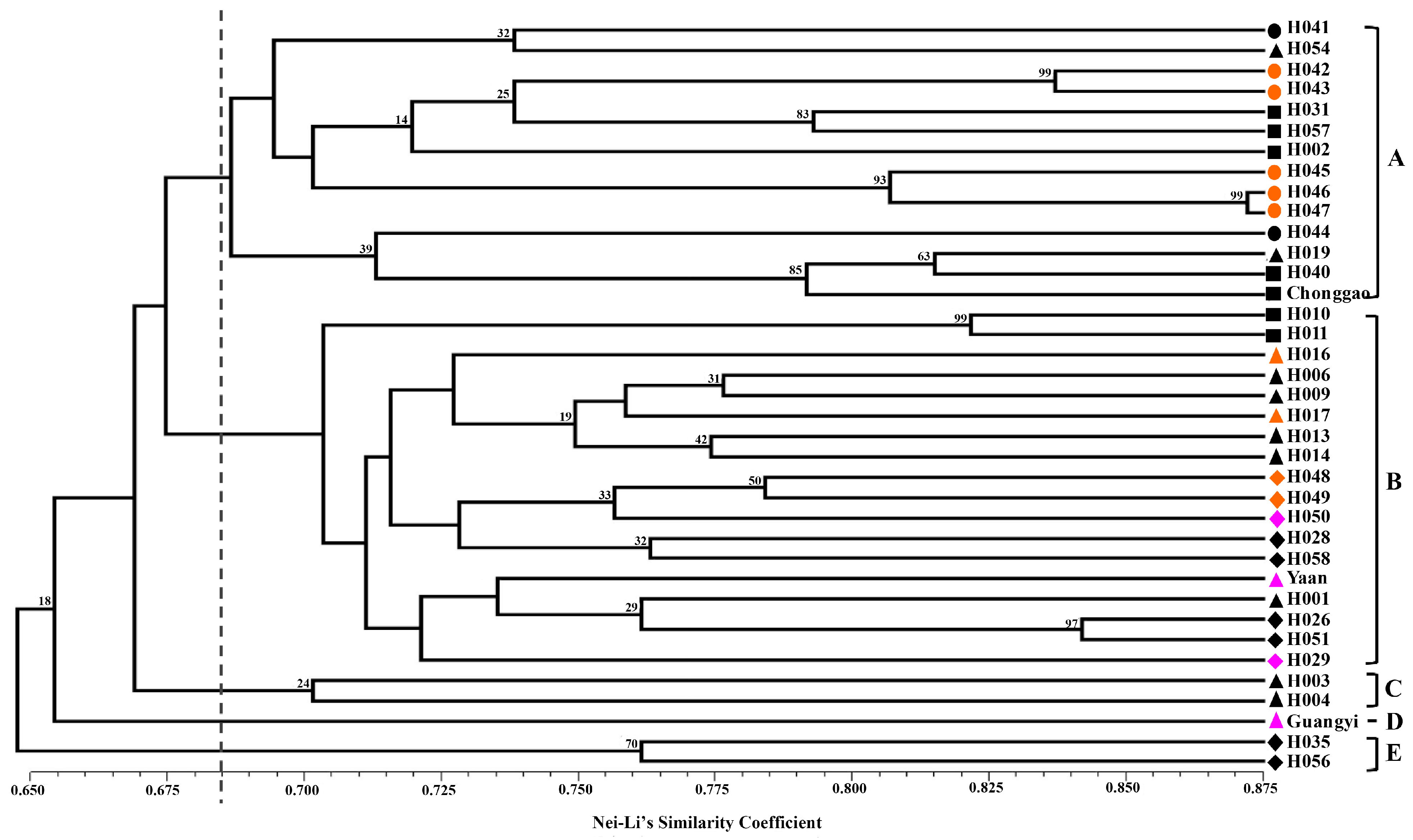
Nei and Li’s GS [40] and the unweighted pair group method with arithmetic mean (UPGMA) were used to perform clustering analysis. The clustering analysis was tested by bootstrapping analysis to assess the robustness of the dendrogram topology using NTSYS-pc 2.10 software [
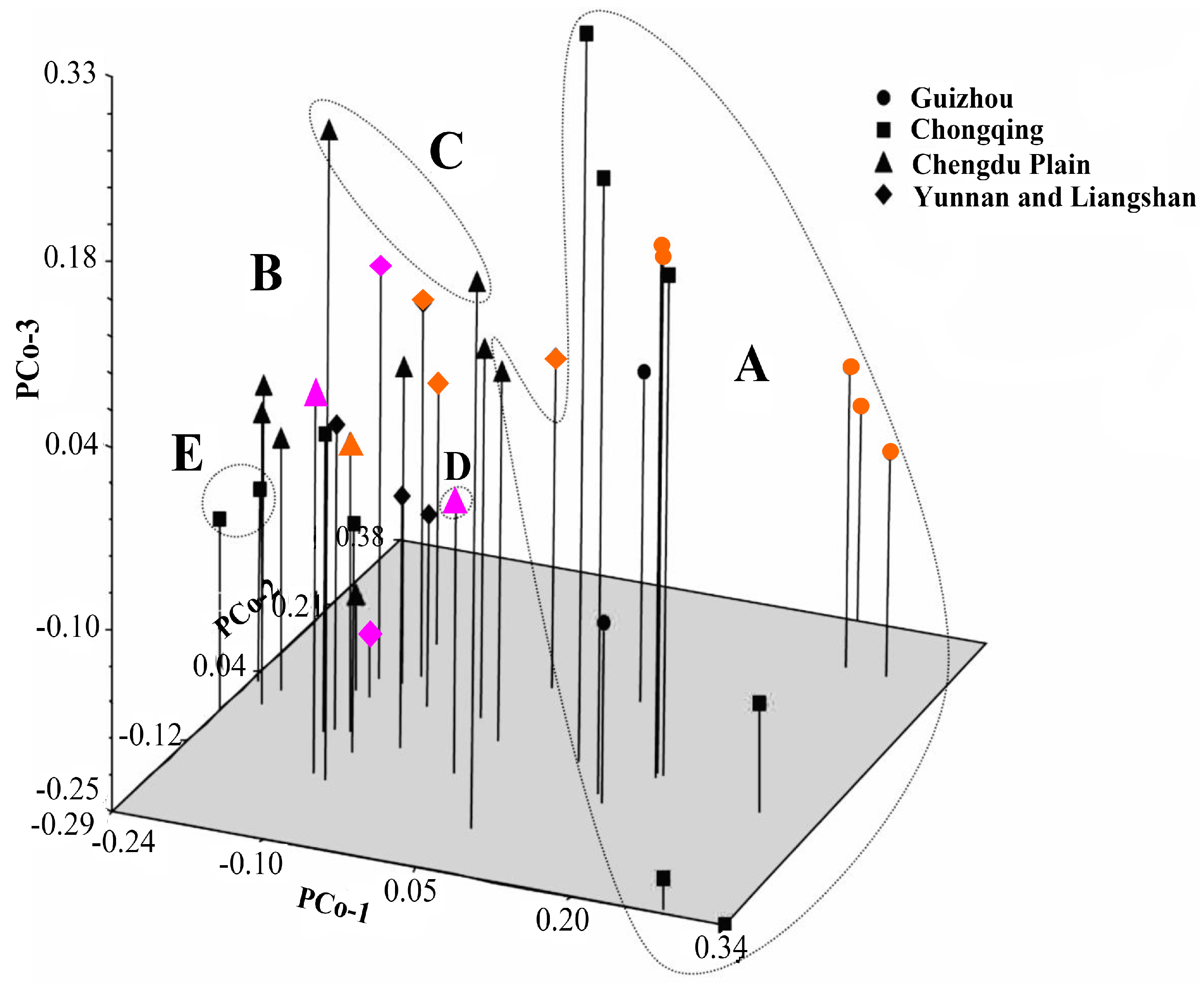
41]. Principal coordinate analysis (PCoA) was also performed to determine the location relationship of the 37 accessions in three dimensions. Furthermore, a Mantel test with 10,000 permutations was conducted using the same software to determine the extent of correlation, if any, between the genetic distance (GD = 1 − GS) and the geographical distance (in kilometers) [42].
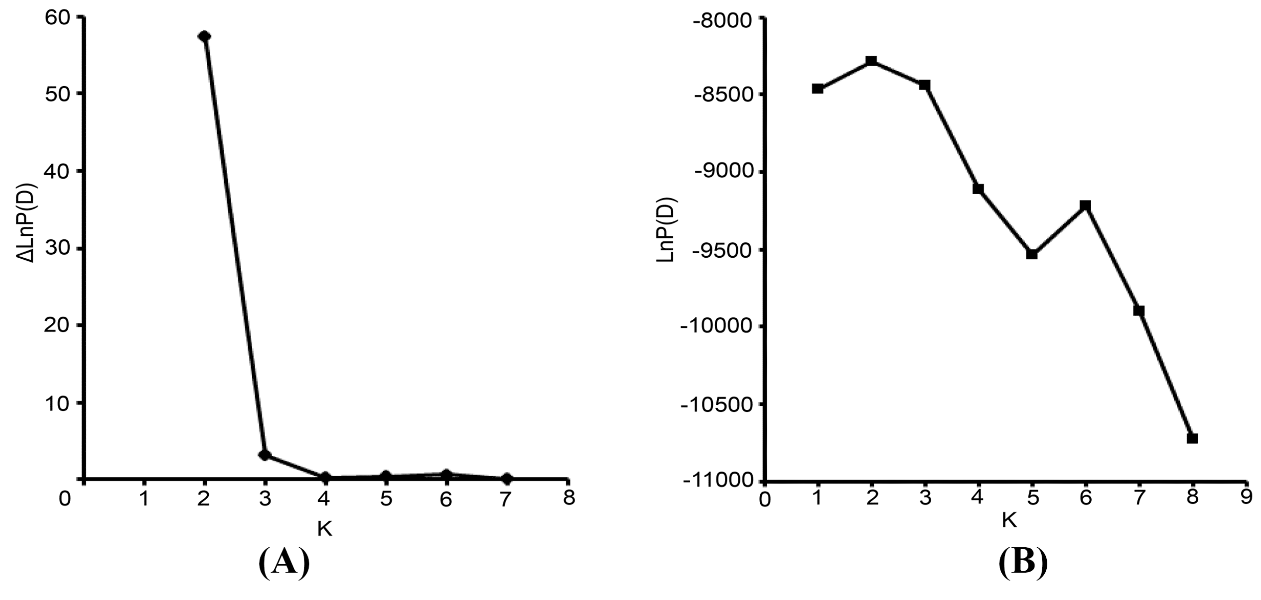
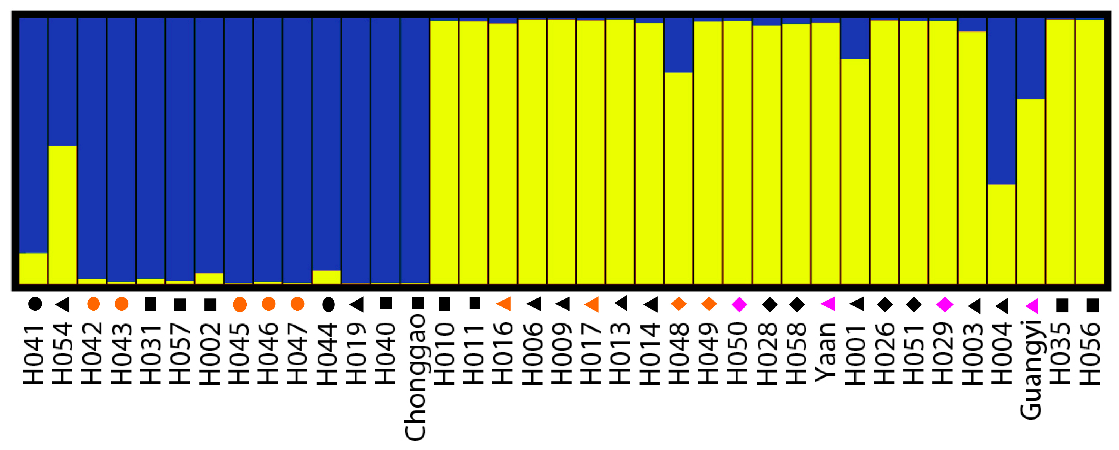
The Bayesian-based clustering method was applied to delineate the clusters of genetically similar accessions using STRUCTURE software version 2.3.3 [18,43]. An admixture model and an allele frequencies-correlated model were adopted without prior assumptions concerning the population. The value of K was set from 1 to 8. Ten independent runs were performed, each with a Markov Chain Monte Carlo (MCMC) of 100,000 repetitions following a burn-in period of 50,000 iterations [17]. Default values were used for all other parameters. For the chosen K value, the run that had the highest likelihood estimate was adopted to assign individuals to clusters. To identify the optimal value of K, the STRUCTURE output file was implemented in Structure Harvester [44]. The 10 runs with the highest LnP(D) and/or ΔLnP(D) values for the selected K-value were retained, and their admixture estimates were averaged using CLUMPP 1.1 [45]. The run with the maximum likelihood was applied to subdivide the tested accessions into different subgroups using a membership probability threshold of 0.60 [46]. Accessions with less than 0.60 membership probabilities were retained in the admixed group (AD). The results were visualized using DISTRUCT 1.1 [47].
The germplasm collections studied here were artificially grouped into four geographic groups. The geographical distances between accessions within the groups varied greatly from tens to hundreds of kilometers. It is difficult to analyze the variance components and their significance levels of genetic variation within and between geographic groups using common software under the Hardy-Weinberg equilibrium assumption. To avoid the complications mentioned above, genetic divergence was analyzed using Shannon’s diversity index, analysis of molecular variance (AMOVA) and Bayesian inference. The magnitude of the genetic variation was determined for each geographical group using Shannon’s diversity index [48]. Shannon’s diversity index is frequently applied in dominant marker data analysis because the index is insensitive to the potential introduction of bias due to undetectable heterozygosity. Total diversity was calculated using the Shannon index with the following equation: HW = −∑fiLnfi, where “fi” is the frequency of an amplified band across all samples. The Shannon index within a subset of data (a geographic group) can be calculated using the following equation: Hzone = −∑fiLnfi, where “fi” is the frequency of an amplified band within a subset. The average diversity between different groups was calculated using the following equation: HA = Hzone = ∑Hzone/n, where n is the number of groups. Thus, HA is the average group diversity over n groups. The intra- and inter-group diversity components were calculated as HA/HW and (HW − HA)/HW, respectively. To compare the levels of diversity detected by different primer sets, the total Shannon diversity was calculated separately for each primer set.
AMOVA based on a Euclidean squared distance matrix was hierarchically calculated to estimate the allocation of genetic variation among and within regional groups using GenAlEx version 6.5 [32]. AMOVA components of variance include ΦPT, an analogue of FST [49]. The significance of the different components of variance was tested with 9999 random permutations.
We compared the Shannon index and AMOVA results for the population genetic structure with allele-frequency estimates calculated using HICKORY software 1.1 [19]. HICKORY employs a Bayesian approach to estimate θB using dominant markers; HICKORY does not assume Hardy-Weinberg equilibrium. Its f and θB are equivalent to the inbreeding coefficient (FIS) and the fixation index (FST) of F-statistics, respectively. The Bayesian estimator of genetic diversity was calculated for each of the following four models: (1) the full model (with non-informative priors for f and θB); (2) f = 0 (assumes no inbreeding); (3) θB = 0 (assumes no population structure); and (4) f-free (allows for the incorporation of uncertainty concerning f into the analysis). We conducted several runs with default sampling parameters (burn-in = 50,000, sample = 250,000, thin = 50) to ensure model convergence. The deviance information criterion (DIC) was used to estimate the fit between the data and a particular model and to choose among models [50].

4. Conclusions

In summary, the results of our study demonstrate a relatively high level of genetic diversity and low levels of genetic differentiation among geographical groups in whipgrass germplasm. The selected primer sets, which revealed high polymorphism among the accessions, might be applied to other closely related species such as H. altissima and H. sibirica. Incorrect identification and the misplacement of labels remain serious problems in maintaining germplasm. This study demonstrates that SCoT analysis is a simple, effective and reliable technique for identifying and maintaining warm-season grass germplasm and could have applications in the assessment of genetic variability in collections of unknown origin, breeding stocks, and/or plant variety protection.

Ethics Statement

This study was approved by the Department of Grassland Science, Animal Science and Technology College, Sichuan Agricultural University. No specific permissions were required for the collection of Hemarthria compressa samples at locations in southwest China because the research was funded by the National Science and Technology Supporting Project of the People’s Republic of China. In addition, no specific permission was required for the field study, which was conducted in an experimental plot on the farm at Sichuan Agricultural University. H. compressa is not an endangered or protected species.

Acknowledgments

We thank all the participants from the Department of Grassland Science at Sichuan Agricultural University for their contributions to this study. This work was supported by the National Science and Technology Supporting Project (#2011BAD17B03) and the Earmarked Fund for the Modern Agro-Industry Technology Research System (#CARS-35-05). The funders had no role in study design, data collection and analysis, decision to publish, or preparation of the manuscript.

Author Contributions

Conceived and designed the experiment: Xiao Ma, Xin-Quan Zhang, Shi-Qie Bai and Yan Fan. Performed the experiment: Zhi-Hui Guo and Kai-Xin Fu. Analyzed the data: Zhi-Hui Guo, Xiao Ma. Contributed reagents/materials/analysis tools: Xiao Ma, Yan Peng, Yan-Hong Yan, Lin-Kai Huang and Wei Liu. Wrote the paper: Zhi-Hui Guo and Xiao Ma.

Conflicts of Interest

The authors declare no conflict of interest.

References

  1. Yang, C.H.; Zhang, X.Q.; Li, X.L.; Du, Y.; Wu, Y.Q. Hemarthria germplasm resources and breeding. Acta Prataculturae Sin. 2004, 13, 7–12. [Google Scholar]
  2. Chen, Y.X.; Zhang, X.Q.; Yang, C.H.; Ma, X.; Liu, J.P. The Study on Morphologic Diversity of Wild Hemarthria compressa from Southwest China. Grassl. China 2005, 27, 78–80. [Google Scholar]
  3. Chen, Y.X.; Zhang, X.Q.; Yang, C.H.; Ma, X.; Huang, L.K.; Liu, Y. Breeding and Cultivation Techniques of A New Variety Hemarthria compressa cv. Ya’an. Chin. J. Grassl. 2012, 34, 109–112. [Google Scholar]
  4. Semagn, K.; Bjørnstad, Å.; Ndjiondjop, M.N. An overview of molecular marker methods for plants. Afr. J. Biotechnol. 2006, 5, 2540–2568. [Google Scholar]
  5. Andersen, J.R.; Lübberstedt, T. Functional markers in plants. Trends Plant Sci. 2003, 8, 554–560. [Google Scholar] [CrossRef] [PubMed]
  6. Fan, Y.; Li, F.; Zhang, X.Q.; Ma, X. Genetic diversity of Hemarthria compressa germplasm detected by inter-simple sequence repeat (ISSR). Acta Prataculturae Sin. 2007, 16, 76–81. [Google Scholar]
  7. Fan, Y.; Xu, Y.D.; Jiang, A.; Wang, P. Genetic Diversity of Hemarthria compressa Germplasms in Southwest China by SRAP. Genomics Appl. Biol. 2010, 29, 63–70. [Google Scholar]
  8. Chen, Y.X.; Zhang, X.Q.; Xie, W.G.; Ma, X.; Liu, Y. Genetic diversity of Hemarthria compressa germplasms from southwestern China based on EST-SSR. Acta Prataculturae Sin. 2011, 20, 245–253. [Google Scholar]
  9. Collard, B.C.Y.; Mackill, D.J. Start Codon Targeted (SCoT) Polymorphism: A Simple, Novel DNA Marker Technique for Generating Gene-Targeted Markers in Plants. Plant Mol. Biol. Rep. 2009, 27, 86–93. [Google Scholar] [CrossRef]
  10. Xiong, F.Q.; Zhong, R.C.; Han, Z.Q.; Jiang, J.; He, L.Q.; Zhuang, W.J.; Tang, R.H. Start codon targeted polymorphism for evaluation of functional genetic variation and relationships in cultivated peanut (Arachis hypogaea L.) genotypes. Mol. Biol. Rep. 2011, 38, 3487–3494. [Google Scholar] [CrossRef] [PubMed]
  11. Luo, C.; He, X.H.; Chen, H.; Hu, Y.; Ou, S.J. Genetic relationship and diversity of Mangifera indica L.: revealed through SCoT analysis. Genet. Resour. Crop Evol. 2012, 59, 1505–1515. [Google Scholar] [CrossRef]
  12. Guo, D.L.; Zhang, J.Y.; Liu, C.H. Genetic diversity in some grape varieties revealed by SCoT analyses. Mol. Biol. Rep. 2012, 39, 5307–5313. [Google Scholar] [CrossRef] [PubMed]
  13. Pakseresht, F.; Talebi, R.; Karami, E. Comparative assessment of ISSR, DAMD and SCoT markers for evaluation of genetic diversity and conservation of landrace chickpea (Cicer arietinum L.) genotypes collected from north-west of Iran. Physiol. Mol. Biol. Plants 2013, 19, 563–574. [Google Scholar] [CrossRef] [PubMed]
  14. Rathore, N.S.; Rai, M.K.; Phulwaria, M.; Rathore, N.; Shekhawat, N.S. Genetic stability in micropropagated Cleome gynandra revealed by SCoT analysis. Acta Physiol. Plant 2014, 36, 555–559. [Google Scholar] [CrossRef]
  15. Cabo, S.; Ferreira, L.; Carvalho, A.; Martins-Lopes, P.; Martín, A.; Lima-Brito, J.E. Potential of Start Codon Targeted (SCoT) markers for DNA fingerprinting of newly synthesized tritordeums and their respective parents. J. Appl. Genet. 2014, 55, 307–312. [Google Scholar] [CrossRef] [PubMed]
  16. Huang, L.K.; Zhang, X.Q.; Ma, X.; Liu, W.; Li, F.; Zeng, B. Genetic differentiation among Hemarthria compressa populations in south China and its genetic relationship with H. japonica. Hereditas 2008, 145, 84–91. [Google Scholar] [CrossRef] [PubMed]
  17. Evanno, G.; Regnaut, S.; Goudet, J. Detecting the number of clusters of individuals using the software STRUCTURE: A simulation study. Mol. Ecol. 2005, 14, 2611–2620. [Google Scholar] [CrossRef] [PubMed]
  18. Pritchard, J.K.; Stephens, M.; Donnelly, P. Inference of population structure using multilocus genotype data. Genetics 2000, 155, 945–959. [Google Scholar] [PubMed]
  19. Holsinger, K.E.; Lewis, P.O.; Dey, D.K. A Bayesian approach to inferring population structure from dominant markers. Mol. Ecol. 2002, 11, 1157–1164. [Google Scholar] [CrossRef] [PubMed]
  20. Gorji, A.M.; Poczai, P.; Polgar, Z.; Taller, J. Efficiency of Arbitrarily Amplified Dominant Markers (SCOT, ISSR and RAPD) for Diagnostic Fingerprinting in Tetraploid Potato. Am. J. Potato Res. 2011, 88, 226–237. [Google Scholar] [CrossRef]
  21. Roldán-Ruiz, I.; Dendauw, J.; Van Bockstaele, E.; Depicker, A.; de Loose, M. AFLP markers reveal high polymorphic rates in ryegrasses (Lolium spp.). Mol. Breed. 2000, 6, 125–134. [Google Scholar] [CrossRef]
  22. De Riek, J.; Calsyn, E.; Everaert, I.; Van Bockstaele, E.; de Loose, M. AFLP based alternatives for the assessment of Distinctness, Uniformity and Stability of sugar beet varieties. Theor. Appl. Genet. 2001, 103, 1254–1265. [Google Scholar] [CrossRef]
  23. Arya, L.; Narayanan, R.K.; Verma, M.; Singh, A.K.; Gupta, V. Genetic diversity and population structure analyses of Morinda tomentosa Heyne, with neutral and gene based markers. Genet. Resour. Crop Evol. 2014, 61, 1469–1479. [Google Scholar] [CrossRef]
  24. Ostrowski, M.F.; David, J.; Santoni, S.; Mckhann, H.; Reboud, X.; Le Corre, V.; Camilleri, C.; Brunel, D.; Bouchez, D.; Faure, B.; et al. Evidence for a large-scale population structure among accessions of Arabidopsis thaliana: Possible causes and consequences for the distribution of linkage disequilibrium. Mol. Ecol. 2006, 15, 1507–1517. [Google Scholar] [CrossRef]
  25. Wu, Y.Q.; Du, Y. Some Reproductive Characteristics of Hemarthria Compressa. J. Sichuan Agric. Univ. 2000, 18, 262–264. [Google Scholar]
  26. Paun, O.; Bateman, R.M.; Fay, M.F.; Hedrén, M.; Civeyrel, L.; Chase, M.W. Stable epigenetic effects impact adaptation in allopolyploid orchids (Dactylorhiza: Orchidaceae). Mol. Biol. Evol. 2010, 27, 2465–2473. [Google Scholar] [CrossRef] [PubMed]
  27. Pirkhezri, M.H.M.E. Genetic diversity in different populations of Matricaria chamomilla L. growing in Southwest of Iran, based on morphological and RAPD markers. Res. J. Med. Plant 2010, 4, 1–13. [Google Scholar] [CrossRef]
  28. Schaal, B.A.; Hayworth, D.A.; Olsen, K.M.; Rauscher, J.T.; Smith, W.A. Phylogeographic studies in plants: Problems and prospects. Mol. Ecol. 1998, 7, 465–474. [Google Scholar] [CrossRef]
  29. Slatkin, M. Gene flow and the geographic structure of natural. Science 1987, 236, 787–792. [Google Scholar] [CrossRef] [PubMed]
  30. Yeh, F.C.; Yang, R.; Boyle, T.B.; Ye, Z.H.; Mao, J.X. POPGENE, the user-friendly shareware for population genetic analysis. University of Alberta: Edmonton, AB, Canada, 1997. [Google Scholar]
  31. Shannon, C.E. A mathematical theory of communication. Bell Syst. Tech. J. 1948, 27, 379–423, 623–656. [Google Scholar] [CrossRef]
  32. Peakall, R.; Smouse, P.E. GenAlEx 6.5: Genetic analysis in Excel. Population genetic software for teaching and research—An update. Bioinformatics 2012, 28, 2537–2539. [Google Scholar] [CrossRef] [PubMed]
  33. Zhao, R.Z. A study of the physico geographical regionalization in southwest region. J. Southwest China Norm. Univers. (Nat. Sci.) 1997, 22, 83–88. [Google Scholar]
  34. He, L.F.; Chen, L.Z.; Yang, C.H.; Shu, S.M.; Li, C.Q. Chromosome Numbers and Karyotype Analysis of Hemarthria compressa. Acta Agrestia Sin. 2011, 33, 89–94. [Google Scholar]
  35. Doyle, J.J. Isolation of plant DNA from fresh tissue. Focus 1990, 12, 13–15. [Google Scholar]
  36. Gillet, E.M. Genetic analysis of nuclear DNA restriction fragment patterns. Genome 1991, 34, 693–703. [Google Scholar] [CrossRef] [PubMed]
  37. McGregor, C.E.; Lambert, C.A.; Greyling, M.M.; Louw, J.H.; Warnich, L. A comparative assessment of DNA fingerprinting techniques (RAPD, ISSR, AFLP and SSR) in tetraploid potato (Solanum tuberosum L.) germplasm. Euphytica 2000, 113, 135–144. [Google Scholar] [CrossRef]
  38. Prevost, A.; Wilkinson, M.J. A new system of comparing PCR primers applied to ISSR fingerprinting of potato cultivars. Theor. Appl. Genet. 1999, 98, 107–112. [Google Scholar] [CrossRef]
  39. Powell, W.; Morgante, M.; Andre, C.; Hanafey, M.; Vogel, J.; Tingey, S.; Rafalski, A. The comparison of RFLP, RAPD, AFLP and SSR (microsatellite) markers for germplasm analysis. Mol. Breed. 1996, 2, 225–238. [Google Scholar] [CrossRef]
  40. Nei, M.; Li, W. Mathematical model for studying genetic variation in terms of restriction endonucleases. Proc. Natl. Acad. Sci. USA 1979, 76, 5269–5273. [Google Scholar] [CrossRef]
  41. Rohlf, F.J. NTSYS-PC, Numerical Taxonomy System for the PC ExeterSoftware; Version 2.1; Applied Biostatistics Inc.: Setauket, NY, USA, 2000. [Google Scholar]
  42. Mantel, N. The detection of disease clustering and a generalized regression approach. Cancer Res. 1967, 27, 209–220. [Google Scholar] [PubMed]
  43. Falush, D.; Stephens, M.; Pritchard, J.K. Inference of population structure using multilocus genotype data: Linked loci and correlated allele frequencies. Genetics 2003, 164, 1567–1587. [Google Scholar] [PubMed]
  44. Earl, D.A. STRUCTURE HARVESTER: A website and program for visualizing STRUCTURE output and implementing the Evanno method. Conserv. Genet. Resour. 2012, 4, 359–361. [Google Scholar] [CrossRef]
  45. Jakobsson, M.; Rosenberg, N.A. CLUMPP: A cluster matching and permutation program for dealing with label switching and multimodality in analysis of population structure. Bioinformatics 2007, 23, 1801–1806. [Google Scholar] [CrossRef] [PubMed]
  46. Chen, X.J.; Min, D.H.; Yasir, T.A.; Hu, Y.G. Genetic diversity, population structure and linkage disequilibrium in elite chinese winter wheat investigated with SSR markers. PLoS One 2012, 7, e44510. [Google Scholar] [CrossRef] [PubMed]
  47. Rosenberg, N.A. DISTRUCT: A program for the graphical display of population structure. Mol. Ecol. Notes 2004, 4, 137–138. [Google Scholar] [CrossRef]
  48. Prashanth, S.R.; Parani, M.; Mohanty, B.P.; Talame, V.; Tuberosa, R.; Parida, A. Genetic diversity in cultivars and landraces of Oryza sativa subsp. indica as revealed by AFLP markers. Genome 2002, 45, 451–459. [Google Scholar] [CrossRef] [PubMed]
  49. Excoffier, L.; Smouse, P.E.; Quattro, J.M. Analysis of molecular variance inferred from metric distances among DNA haplotypes: Application to human mitochondrial DNA restriction data. Genetics 1992, 131, 479–491. [Google Scholar] [PubMed]
  50. Holsinger, K.E.; Wallace, L.E. Bayesian approaches for the analysis of population genetic structure: An example from Platanthera leucophaea (Orchidaceae). Mol. Ecol. 2004, 13, 887–894. [Google Scholar] [CrossRef] [PubMed]
  • Sample Availability: Samples of the compounds are available from the authors.

