Inter-Dye Distance Distributions Studied by a Combination of Single-Molecule FRET-Filtered Lifetime Measurements and a Weighted Accessible Volume (wAV) Algorithm

Abstract
:
1. Introduction
2. Results and Discussion
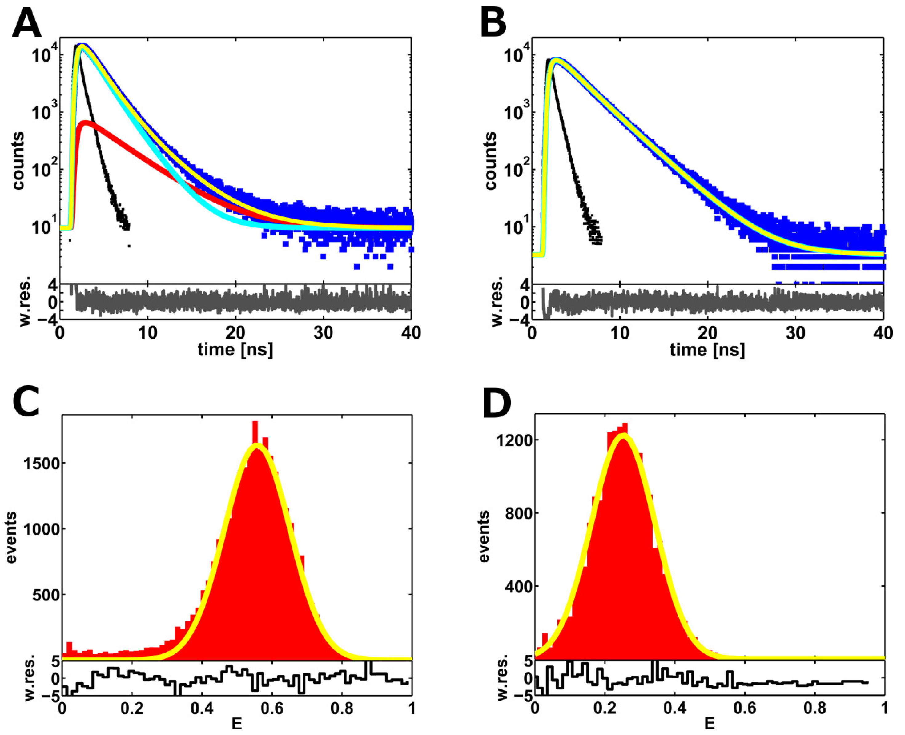
2.1. Ensemble Lifetime FRET Measurements


| Sample | Measurement | 〈RDA〉 [Å] | σDA [Å] | xD0 [%] | |
|---|---|---|---|---|---|
| 10 bp DNA | ensemble | 46.2 ± 0.2 | 7.1 ± 0.3 | 16.0 ± 0.3 | 1.033 |
| 10 bp DNA | smFRET filtered | 49.1 ± 0.2 | 4.5 ± 0.4 | 4.8 ± 0.4 | 1.123 |
| 17 bp DNA | ensemble | 60.0 ± 0.3 | 5.9 ± 0.5 | 18.2 ± 1.1 | 0.999 |
| 17 bp DNA | smFRET filtered | 62.7 ± 0.2 | 7.2 ± 0.5 | 0 | 1.075 |

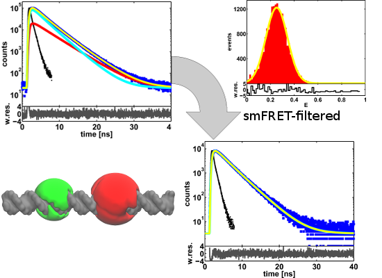
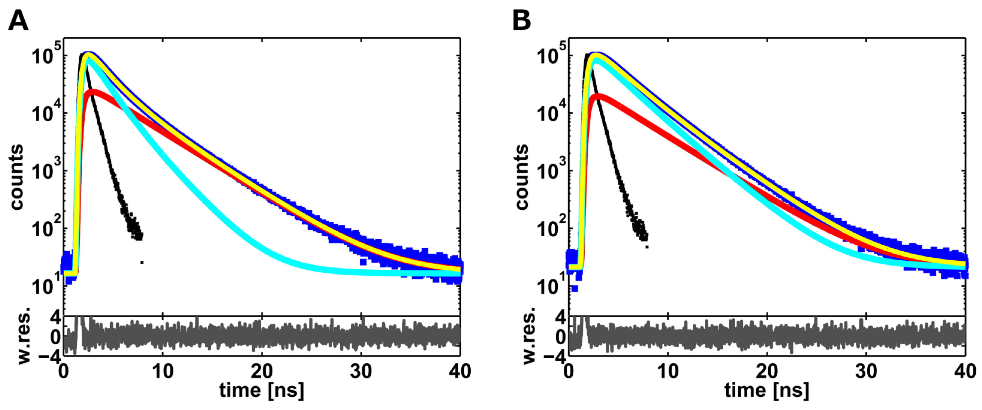
2.2. Single-Molecule FRET-Filtered Lifetime Measurements

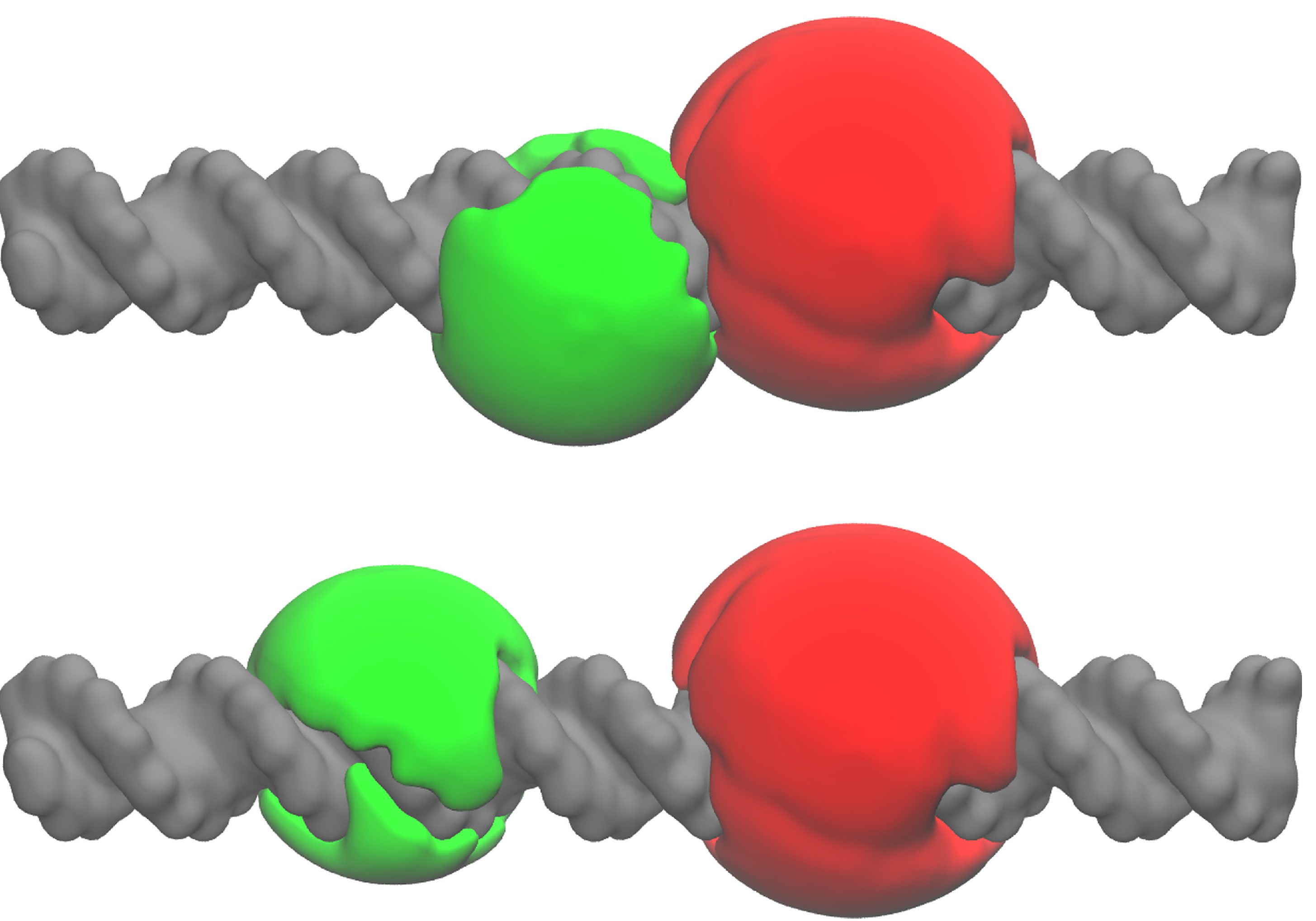
2.3. A Weighted Accessible Volume Algorithm (wAV)

3. Experimental Section
3.1. Sample Preparation
3.2. Experimental Set-Up
3.3. Ensemble Lifetime Measurements
3.4. Single-Molecule Measurements
| Sample | 𝜏1 | 𝜏2 | x1 | ɸ | |
|---|---|---|---|---|---|
| D0-dsDNA (10 bp) | 4.06 ns | 1.38 ns | 0.94 | 1.07 | 0.90 |
| D0-dsDNA (17 bp) | 4.09 ns | 1.52 ns | 0.91 | 1.04 | 0.88 |
| A0-dsDNA (10 bp and 17 bp) | 1.38 ns | 0.88 ns | 0.28 | 1.10 | 0.32 |
| Alexa 488-NHS | 4.025 ns | - | 1 | 1.13 | 0.92 |
| Alexa 647-NHS | 1.053 ns | - | 1 | 1.80 | 0.33 |
3.5. Data Analysis
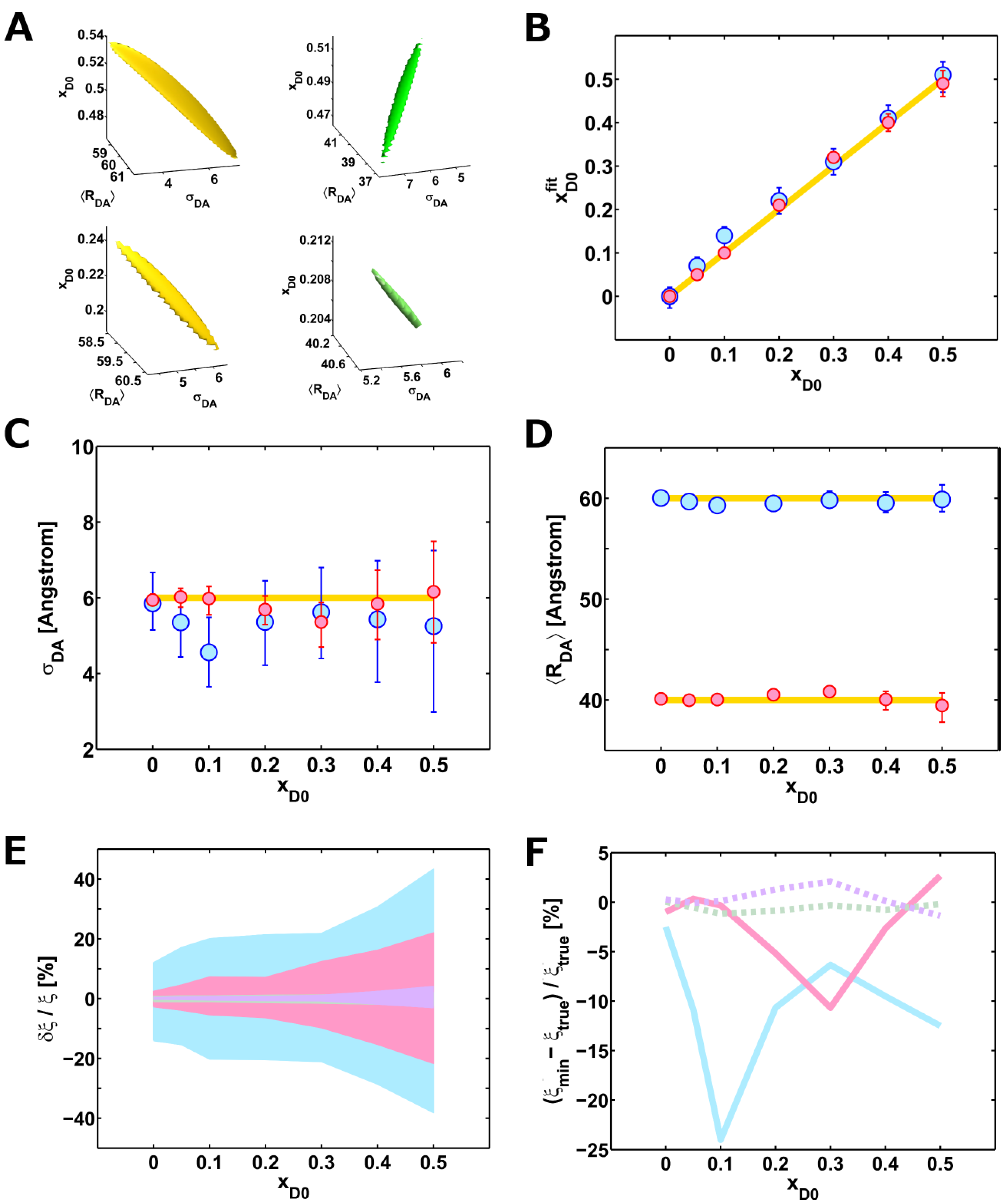
3.6. Error Analysis
3.7. Generation of Artificial Lifetime Decays
3.8. Weighted Accessible Volume Algorithm
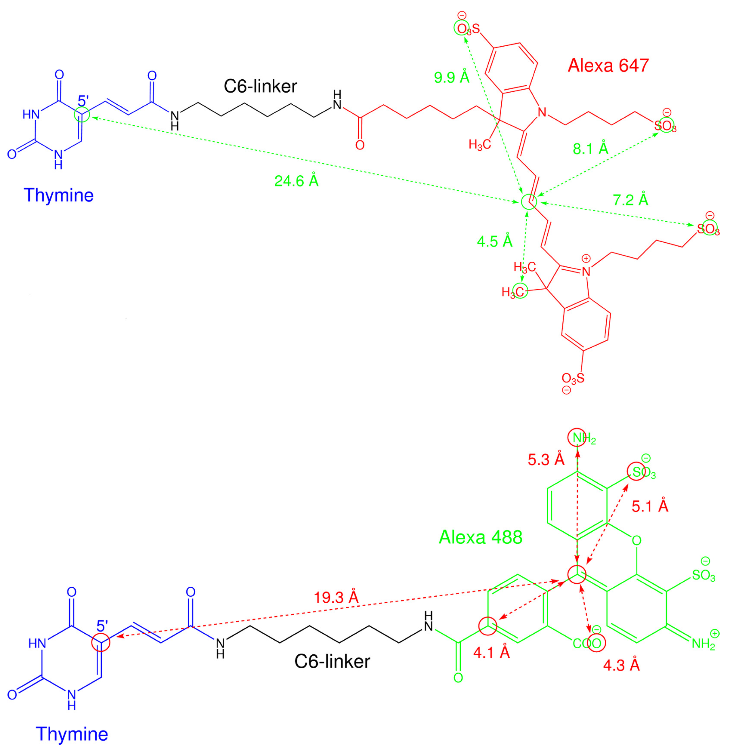
| Dye | Llink | wlink | Rdye,1 | Rdye,2 | Rdye,3 |
|---|---|---|---|---|---|
| T-C6-Alexa 488 | 19.3 Å | 4.5 Å | 5.2 Å | 4.2 Å | 1.5 Å |
| T-C6-Alexa 647 | 24.6 Å | 4.5 Å | 9.9 Å | 7.7 Å | 1.5 Å |
4. Conclusions
Acknowledgments
Author Contributions
Appendix
| (%) | I0 (counts) | BG (counts) | xD0 (%) | 〈 RDA〉 (Å) | (Å) | |
|---|---|---|---|---|---|---|
| 50 | 9,999 | 18.8 | 49 (46 – – 52) | 39.5 (37.8 – – 40.7) | 6.2 (4.8 – – 7.5) | 1.097 |
| 40 | 10,005 | 18.8 | 40 (38 – – 42) | 40.1 (39.0 – – 40.1) | 5.8 (4.8 – – 7.5) | 1.080 |
| 30 | 9,998 | 19.3 | 32 (31 – – 33) | 40.8 (40.3 – – 41.2) | 5.4 (4.7 – – 5.9) | 1.032 |
| 20 | 9,986 | 18.8 | 21 (20 – – 21) | 40.5 (40.2 – – 40.1) | 5.7 (5.3 – – 6.1) | 1.049 |
| 10 | 9,974 | 18.9 | 10 (9.6 – – 10.3) | 40.0 (39.7 – – 40.3) | 6.0 (5.6 – – 6.3) | 1.019 |
| 5 | 9,986 | 18.8 | 5 (4.9 – – 5.2) | 39.9 (39.7 – – 40.2) | 6.0 (5.8 – – 6.3) | 1.0092 |
| 0 | 10,028 | 19.0 | 0 (0.0 – – 0.0) | 40.1 (39.8 – – 40.3) | 5.9 (5.8 – – 6.1) | 1.0025 |
| true values | 10,000 | 20 | / | 40.0 | 6.0 | / |
| (%) | I0 (counts) | BG (counts) | xD0 (%) | 〈 RDA〉 (Å) | (Å) | |
|---|---|---|---|---|---|---|
| 50 | 9,997 | 19.1 | 51 (47 – – 54) | 59.9 (58.7 – – 61.3) | 5.3 (3.0 – – 7.3) | 1.019 |
| 40 | 10,001 | 18.8 | 41 (38 – – 44) | 59.5 (58.6 – – 60.6) | 5.4 (3.8 – – 7.0) | 1.050 |
| 30 | 10,004 | 19.0 | 31 (28 – – 34) | 59.8 (59.1 – – 60.7) | 5.6 (4.4 – – 6.8) | 1.008 |
| 20 | 10,011 | 18.8 | 22 (19 – – 25) | 59.5 (58.9 – – 60.3) | 5.4 (4.2 – – 6.5) | 1.037 |
| 10 | 9,986 | 18.6 | 14 (11 – – 16) | 59.3 (58.8 – – 59.9) | 4.6 (3.7 – – 5.5) | 1.041 |
| 5 | 9,992 | 18.7 | 7 (4 .6 – – 9.0) | 59.7 (59.2 – – 60.3) | 5.4 (4.4 – – 6.2) | 1.037 |
| 0 | 9,992 | 18.8 | 0 (– 0.3 – – 0.2) | 60.0 (59.6 – – 60.6) | 5.9 (5.2 – – 6.7) | 1.041 |
| true values | 10,000 | 20 | / | 60.0 | 6.0 | / |
Conflicts of Interest
References
- Lakowicz, J.R. Principles of Fluorescence Spectroscopy,, 2nd ed.; Kluwert Academic/Plenum Publ.: New York, NY, USA, 1999. [Google Scholar]
- Förster, T. Zwischenmolekulare Energiewanderung und Fluoreszenz. Ann. Phys. 1948, 6, 55–75. [Google Scholar] [CrossRef]
- Grinvald, A.; Haas, E.; Steinberg, I.Z. Evaluation of the distribution of distances between energy donors and acceptors by fluorescence decay. Proc. Natl. Acad. Sci. USA 1972, 69, 2273–2277. [Google Scholar] [CrossRef] [PubMed]
- Beechem, J.M.; Haas, E. Simultaneous determination of intramolecular distance distributions and conformational dynamics by global analysis of energy transfer measurements. Biophys. J. 1989, 55, 1225–1236. [Google Scholar] [CrossRef] [PubMed]
- Haran, G.; Haas, E.; Szpikowska, B.K.; Mas, M.T. Domain motions in phosphoglycerate kinase: Determination of inter-domain distance distributions by site-specific labeling and time-resolved fluorescence energy transfer. Proc. Natl. Acad. Sci. USA 1992, 89, 11764–11768. [Google Scholar] [CrossRef] [PubMed]
- Lillo, M.P.; Beechem, J.M. Design and characterization of a multisite fluorescence energy-transfer system for protein folding: A steady-state and time-resolved study of yeast phosphoglycerate kinase. Biochemistry 1997, 36, 11261–11272. [Google Scholar] [CrossRef] [PubMed]
- McWerther, C.A.; Haas, E.; Leed, A.R.; Scheraga, H.A. Conformational unfolding in the N-terminal region of ribonuclease A detected by nonradiative energy transfer. Biochemistry 1986, 25, 1951–1963. [Google Scholar] [CrossRef] [PubMed]
- Haas, E.; Wilchek, M.; Katchalski-Katzir, E.; Steinberg, I.Z. Distribution of end-to-end distances of oligopeptides in solution as estimated by energy transfer. Proc. Natl. Acad. Sci. USA 1975, 72, 1807–1811. [Google Scholar] [CrossRef] [PubMed]
- Sindbert, S.; Kalinin, S.; Nguyen, H.; Kienzler, A.; Clima, L.; Bannwarth, W.; Appel, B.; Müller, S.; Seidel, C.A.M. Accurate distance determination of nucleic acids via Förster resonance energy transfer: Implications of dye linker length and rigidity. J. Am. Chem. Soc. 2011, 133, 2463–2480. [Google Scholar] [CrossRef] [PubMed]
- Gopich, I.V.; Szabo, A. Single-molecule FRET with diffusion and conformational dynamics. J. Phys. Chem. B 2007, 111, 12925–12932. [Google Scholar] [CrossRef] [PubMed]
- Hoefling, M.; Lima, N.; Haenni, D.; Seidel, C.A.M.; Schuler, B.; Grubmüller, H. Structural heterogeneity and quantitative FRET efficiency distributions of polyprolines through a hybrid atomistic simulation and Monte Carlo approach. PLoS One 2011, 6, e19791. [Google Scholar] [CrossRef] [PubMed] [Green Version]
- Sindbert, S. FRET Restrained High-Precision Structural Modeling of Biomolecules. Ph.D. Thesis, Heinrich Heine Universität, Düsseldorf, Germany, 2012. [Google Scholar]
- Woz´niak, A.K.; Schröder, G.; Grubmüller, H.; Seidel, C.A.M.; Osterhelt, F. Single-molecule FRET measures bends and kinks in DNA. Proc. Natl. Acad. Sci. USA 2008, 105, 18337–18342. [Google Scholar] [CrossRef] [PubMed]
- Merchant, K.A.; Best, R.B.; Louis, J.M.; Gopich, I.V.; Eaton, W.A. Characterizing the unfolded states of proteins using single-molecule FRET spectroscopy and molecular simulations. Proc. Natl. Acad. Sci. USA 2007, 104, 1528–1533. [Google Scholar] [CrossRef] [PubMed]
- Kalinin, S.; Peulen, T.; Sindbert, S.; Rothwell, P.J.; Berger, S.; Restle, T.; Goody, R.S.; Gohlke, H.; Seidel, C.A.M. A toolkit and benchmark study for FRET-restrained high-precision structural modeling. Nat. Methods 2012, 9, 1218–1225. [Google Scholar] [CrossRef] [PubMed]
- Muschielok, A.; Andrecka, J.; Jawhari, A.; Brückner, F.; Cramer, P.; Michaelis, J. A nano-positioning system for macromolecular structural analysis. Nat. Methods 2008, 5, 965–971. [Google Scholar] [CrossRef] [PubMed]
- Gabba, M.; Poblete, S.; Rosenkranz, T.; Katranidis, A.; Kempe, D.; Züchner, T.; Winkler, R.G.; Gompper, G.; Fitter, J. Conformational state distributions and catalytically relevant dynamics of a hinge-bending enzyme studied by single-molecule FRET and a coarse-grained simulation. Biophys. J. 2014, 107, 1913–1923. [Google Scholar] [CrossRef] [PubMed]
- Smith, S.B.; Cui, Y.; Bustamante, C. Overstretching b-DNA: The elastic response of individual double-stranded and single-stranded DNA molecules. Science 1996, 271, 795–799. [Google Scholar] [CrossRef] [PubMed]
- Müller, B.K.; Zaychikov, E.; Bräuchle, C.; Lamb, D.C. Pulsed interleaved excitation. Biophys. J. 2005, 89, 3508–3522. [Google Scholar] [CrossRef]
- Schröder, G.U.; Alexiev, U.; Grubmüller, H. Simulation of fluorescence anysotropy experiments: Probing protein dynamics. Biophys. J. 2005, 89, 3757–3770. [Google Scholar] [CrossRef] [PubMed]
- Fisz, J.J. Fluorescence polarization spectroscopy at combined high-aperture excitation and detection: Application to one-photon-excitation fluorescence microscopy. J. Phys. Chem. A 2007, 111, 8606–8621. [Google Scholar] [CrossRef] [PubMed]
- Unruh, J.R.; Gokulrangan, G.; Lushington, G.H.; Johnason, C.K.; Wilson, G.S. Orientational dynamics and dye-DNA interactions in a dye-labeled DNA aptamer. Biophys. J. 2005, 88, 3455–3465. [Google Scholar] [CrossRef] [PubMed]
- Sanborn, M.E.; Connolly, B.K.; Gurunathan, K.; Levitus, M. Fluorescence properties and photophysics of the sulfoindocyanine Cy3 linker covalently to DNA. J. Phys. Chem. B 2007, 111, 11064–11074. [Google Scholar] [CrossRef]
- Allodi, G. FMINUIT—A Binding to Minuit for Matlab, Octave & Scilab. 2010. Available online: http://www.fis.unipr.it/giuseppe.allodi/Fminuit (accessed on 11 November 2014).
- Gopich, I.V. Concentration effects in “single-molecule” spectroscopy. J. Phys. Chem. B 2008, 112, 6214–6220. [Google Scholar] [CrossRef] [PubMed]
- Nir, E.; Michalet, X.; Hamadani, K.M.; Laurence, T.A.; Neuhauser, D.; Kovchegov, Y.; Weiss, S. Shot-noise single-molecule FRET histograms: Comparison between theory and experiments. J. Phys. Chem. B 2006, 110, 22103–22124. [Google Scholar] [CrossRef] [PubMed]
- Chen, H.; Ahsan, S.S.; Santiago-Berrios, M.B.; Abruña, H.D.; Webb, W.W. Mechanisms of quenching of Alexa fluorophores by natural amino acids. J. Am. Chem. Soc. 2010, 132, 7244–7245. [Google Scholar] [CrossRef] [PubMed]
- Vaiana, A.C.; Neuweiler, H.; Schulz, A.; Wolfrum, J.; Sauer, M.; Smith, J.C. Fluorescence quenching of dyes by tryptophan: Interactions of atomic detail from combination of experiment and computer simulation. J. Am. Chem. Soc. 2003, 125, 14564–14572. [Google Scholar] [CrossRef] [PubMed]
- Kalinin, S.; Sisamakis, E.; Magennis, S.W.; Felekyan, S.; Seidel, C.A.M. On the origin of broadening of single-molecule FRET efficiency distributions beyond shot noise limits. J. Phys. Chem. B 2010, 114, 6197–6206. [Google Scholar] [CrossRef]
- Van Dijk, M.; Bonvin, A.M. 3D-DART: A DNA structure modelling server. Nucleic Acids Res. 2009, 37, W235–W239. [Google Scholar] [CrossRef] [PubMed]
- Richter, D. Flexible Polymers. In Lecture Notes: Macromolecular Systems in Soft and Living Matter, Proceedings of the 42nd IFF Springschool, Forschungszentrum, Jülich, Jülich, Germany, 14–25 February 2011.
- Wahl, M. Time-Correlated Single Photon Counting; Technical Note; PicoQuant: Berlin, Germany, 2014. [Google Scholar]
- Luchowski, R.; Gryczynski, Z.; Sarkar, P.; Borejdo, J.; Szabelski, M.; Kapusta, P.; Gryczynski, I. Instrument response standard in time-resolved fluorescence. Rev. Sci. Instrum. 2009, 80, 033109. [Google Scholar] [CrossRef] [PubMed]
- Szabelski, M.; Luchowski, R.; Gryczynski, Z.; Kapusta, P.; Ortmann, U.; Gryczynski, I. Evaluation of instrument response functions for lifetime imaging detectors using quenched Rose Bengal solutions. Chem. Phys. Lett. 2009, 471, 153–159. [Google Scholar] [CrossRef]
- Fries, J.; Brand, L.; Eggeling, C.; Köllner, M.; Seidel, C.A.M. Quantitative Identification of Different Single Molecules by Selective Time-Resolved Confocal Fluorescence Spectroscopy. J. Phys. Chem. A 1998, 102, 6601–6613. [Google Scholar] [CrossRef]
- Zhang, K.; Yang, H. Photon-by-photon determination of emission bursts from diffusing single chromophores. J. Phys. Chem. B 2005, 109, 21930–21937. [Google Scholar] [CrossRef] [PubMed]
- Sisamakis, E.; Valeri, A.; Kalinin, S.; Rothwell, P.J.; Seidel, C.A.M. Accurate single-molecule FRET studies using multiparameter fluorescence detection. Methods Enzymol. 2010, 575, 455–514. [Google Scholar]
- Wolberg, J. Data Analysis Using the Method of Least Squares; Springer: Berlin/Heidelberg, Germany, 2006. [Google Scholar]
- Kempe, D. Time Resolve Fluorescence Studies on Proteins: Measurements and Data Analysis of Anisotropy Decays and Single Molecule FRET Efficiencies. Master’s Thesis, University of Cologne, Cologne, Germany, February 2012. [Google Scholar]
- Beechem, J.M. Global analysis of biochemical and biophysical data. Methods Enzymol. 1992, 210, 37–54. [Google Scholar] [PubMed]
- Vöpel, T.; Hengstenberg, C.S.; Peulen, T.O.; Ajaj, Y.; Seidel, C.A.M.; Herrmann, C.; Klare, J.P. Triphosphate induced dimerization of human guanylate binding protein 1 involves association of the C-terminal helices: A joint double electron-electron resonance and FRET study. Biochemistry 2014, 53, 4590–4600. [Google Scholar] [CrossRef]
- Nettels, D.; Hoffmann, A.; Schuler, B. Unfolded protein and peptide dynamics investigated with single-molecule FRET and correlation spectroscopy from picoseconds to seconds. J. Phys. Chem. B 2008, 112, 6173–6146. [Google Scholar] [CrossRef]
- Sample Availability: Fluorescently labeled single DNA strands are commercially available from PURIMEX (Grebenstein, Germany) while the complementary unlabeled strands were purchased from Eurofins MWG Operon (Ebersberg, Germany).
© 2014 by the authors. Licensee MDPI, Basel, Switzerland. This article is an open access article distributed under the terms and conditions of the Creative Commons Attribution license ( http://creativecommons.org/licenses/by/4.0/).
Share and Cite
Höfig, H.; Gabba, M.; Poblete, S.; Kempe, D.; Fitter, J. Inter-Dye Distance Distributions Studied by a Combination of Single-Molecule FRET-Filtered Lifetime Measurements and a Weighted Accessible Volume (wAV) Algorithm. Molecules 2014, 19, 19269-19291. https://doi.org/10.3390/molecules191219269
Höfig H, Gabba M, Poblete S, Kempe D, Fitter J. Inter-Dye Distance Distributions Studied by a Combination of Single-Molecule FRET-Filtered Lifetime Measurements and a Weighted Accessible Volume (wAV) Algorithm. Molecules. 2014; 19(12):19269-19291. https://doi.org/10.3390/molecules191219269
Chicago/Turabian StyleHöfig, Henning, Matteo Gabba, Simón Poblete, Daryan Kempe, and Jörg Fitter. 2014. "Inter-Dye Distance Distributions Studied by a Combination of Single-Molecule FRET-Filtered Lifetime Measurements and a Weighted Accessible Volume (wAV) Algorithm" Molecules 19, no. 12: 19269-19291. https://doi.org/10.3390/molecules191219269