From Randomness to Order

Abstract

I review some selected situations in which order builds up from randomness, or a losing trend turns into winning. Except for Section 4 (which is mine), all cases are well documented and the price paid to achieve order is apparent.

1. Introduction

One statement of the second law of thermodynamics is that, "randomness never decreases". In order to be meaningful, this statement has to be defined precisely. Careful definitions can be found in many references; some of them, selected according to a very personal taste, are listed in Ref. [1]. In this paper I review some attempts to create order out of randomness, and discuss their thermodynamic implications.

2. Smoluchowski's Trapdoor

Long ago, Smoluchowski [2] proposed an automated version of Maxwell's demon. Following Smoluchowski's ideas, Skordos and Zurek [3] studied the model depicted in Fig. 1. Two chambers contain circular molecules. The molecules can pass from one chamber to the other through an orifice, but then they meet an obstacle: a vertical piston that can move horizontally. The motion of the piston is constrained by ideal rails (dashed lines) along which it can slide. When the piston reaches an end of the rails, it bounces back. The molecules are initially assigned random velocities and afterwards all the

Figure 1. Model considered in Ref. [3]. The dashed lines are transparent to the molecules and rigid to the piston.

Figure 1. Model considered in Ref. [3]. The dashed lines are transparent to the molecules and rigid to the piston.

objects move at constant velocities until they collide. All collisions between any two objects are elastic.

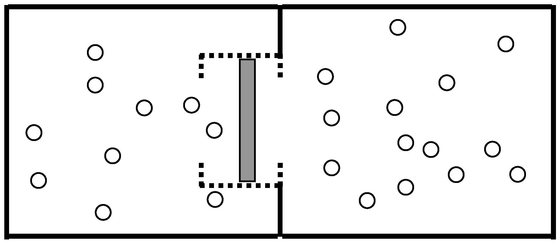
This piston is intended to act as a rectifier: if a molecule hits it from the right, the collision tends to open the entrance and the particle will have a large probability to leak into the left chamber; if the piston is hit from the left, it will be pushed towards the orifice and obstruct it.

Numeric simulations show that the piston indeed acts as a rectifier: if a low density at the left is maintained by replacing the collisions at the left wall by periodic boundary conditions between the outer walls, we obtain a net flow to the left; this flow is much larger than the flow to the right that is obtained in the reversed situation. Also, if we initially locate all the molecules at the left chamber, the time required to reach equilibrium is much longer than the equilibration time when we start from the right chamber.

However, when equilibrium is reached, the average density of molecules is the same in both chambers (provided that the volume occupied by the piston is accounted for). This result may seem paradoxical, since we expected the piston to be a bigger obstacle to particles coming from the left than to their counterparts from the right. Our expectation doesn't work because the piston has thermal fluctuations too. Therefore, it sometimes kicks molecules into the right chamber, precisely in the amount required to cancel the rectifying effect.

In order to have a net rectifying effect we can "cool" the piston: at given periods of time the velocity of the piston is multiplied by a factor smaller than 1, and the energy taken from the piston is distributed among all the molecules. In this way we can indeed start from equal densities in both chambers and a larger density will build up at the left. But since an external agent has to transfer heat from the cold piston to the hot molecules, the decrease in entropy of the system is not a threat to the second law.

An earlier study [4] considered a model with the same mechanical features as in Fig. 1, but this time a subtler deviation from randomness was searched for. In this case there was only one chamber, and the rails were impermeable to the molecules. The velocity distribution of the piston was imposed by an external heat reservoir and the molecules were assumed to have a mean free path much longer than the dimensions of the chamber, so that their velocity distribution was imposed by the piston.

The heuristics for this model were as follows: let's assume that, in agreement with the laws of thermodynamics and statistical mechanics, the piston velocities have the Maxwell-Boltzmann distribution. The particles acquire their velocity distribution only as they collide with the piston. But those particles with a large velocity meet the piston again after a relatively short time (and hence acquire a new velocity), whereas slow particles keep their velocities for a long time, and therefore have a large statistical weight. Therefore we might expect that, when equilibrium is reached, the velocity distribution for the particles will not be that of Maxwell-Boltzmann, but rather a distribution with higher weights to lower velocities. And any distribution which is not that of Maxwell-Boltzmann implies a greater order than that predicted by thermodynamics and statistical mechanics in this situation.

The flaw in the previous argument is that when a particle acquires a small velocity after colliding with the piston, it stays for a relatively long time in the region where the piston is allowed to move. This gives the piston another opportunity to kick the particle again and increase its velocity. This second collision exactly balances the statistics, so that the equilibrium distribution for the particles is that of Maxwell-Boltzmann after all.

3. Brownian Motors

Let us consider a one-dimensional particle that moves under the influence of three agents: Brownian bombardment, viscosity (which might be a consequence of Brownian bombardment) and an externally applied force, which can be derived from a potential as sketched in Fig. 2. The potential will vary in time. Situations of this kind have been widely studied during the last decade, theoretically and

Figure 2. Potential energy of the particle, as a function of position, at some fixed time.

Figure 2. Potential energy of the particle, as a function of position, at some fixed time.

experimentally [5].

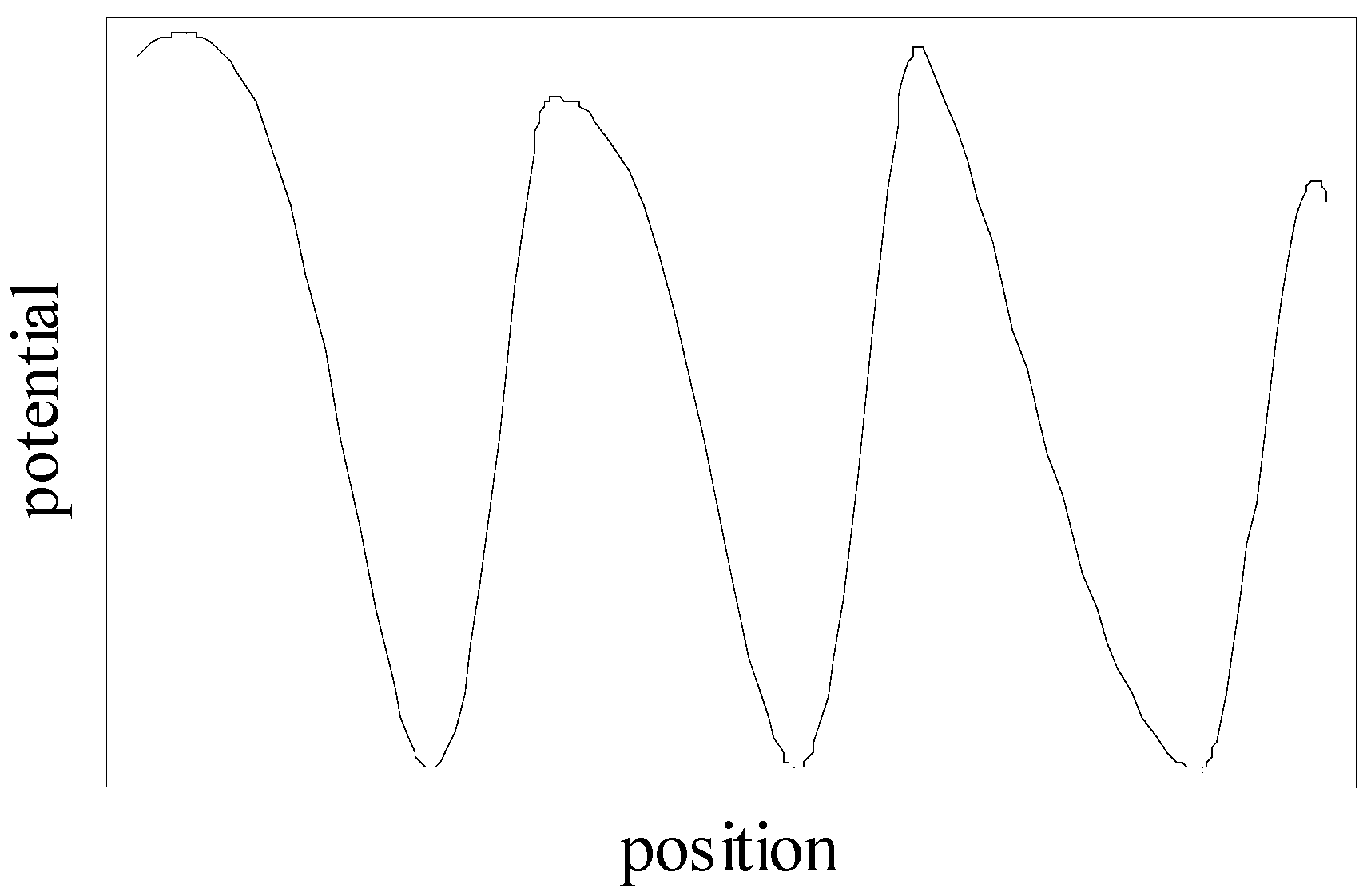
In order to have a definite picture in mind, let's assume that the shape of the potential remains fixed, but its size oscillates as a function of time. We will require three basic properties from the potential: first, it has an unlimited number of minima and maxima; second, for every minimum, the closest maximum will be located at its right; third, when the potential has its full size, the height of the potential barriers will be large compared with Brownian energies.

If the potential remains close to its full size during a period of time which is not too short, the force that it produces, together with viscosity, will push the particle into some minimum, and Brownian bombardment will cause small fluctuations around this minimum. But at some later time the potential barriers will be smaller than the energy of typical fluctuations and, if this situation persists long enough, the particle will diffuse over a barrier to a neighboring minimum. Since the highest obstacle at the right is closer than that at the left, the probability of diffusing to the right is larger and therefore, on the average, the particle will flow to the right. This will happen even if the energy of the particle increases (at a reasonable rate) as it flows to the right.

The optimal lapse of time during which the barriers remain low should be such that the particle has a considerable probability of diffusing to the right and just a minute probability of diffusing to the left. But even if the barriers are low during a very long time, our "motor" would still work: without the influence of the barriers, the particle diffuses in either direction with equal probabilities; then, when the potential becomes large, there is a larger probability that the particle will be located at a position where the slope is negative, and the particle will be pushed to the right.

The final result is that we have found an ordered motion of the particle (to the right) that would not occur without the random Brownian hits. In this sense we may claim that ordered motion has been taken from randomness. To achieve this, we also need an asymmetric potential that varies in time. The time dependence of the potential can also be quite random, provided that the barriers are "on" and "off" during sufficiently long times. This rectification of Brownian motion doesn't mean that the second law is violated, since, every time the potential is turned on, it performs work on the particle.

As a closing remark I review the case in which the potential is symmetric and independent of time. In this case there is no reason for drift in a preferred direction. But random noise can still play a constructive role: if an additional small force, periodic in time, is exerted on the particle, the response of the particle can be enhanced by the presence of an appropriate amount of noise. This phenomenon is known as "stochastic resonance" [6].

4. Asymmetric Superconducting Loop

We consider now an asymmetric superconducting loop that encloses a magnetic flux Φ, as in Fig. 3. Since we will consider fluctuations in this system, an appropriate theory for its description would be the time-dependent Ginzburg-Landau model [7]. Thus far, I have not treated this problem using this theory; instead [8], I have modeled each segment as if it were a Josephson junction [7]. In this case the current I_i that flows through the segment i can be written in the form

I_i = I_cif_i(γ_i) + I_Ri + I_Ni,

Where I_cif_i(γ_i) is the supercurrent, I_Ri is the normal current according to Ohm's law and I_Ni is the

Figure 3. Superconducting loop, composed of two unequal segments, that encloses a magnetic flux Φ. V is the average voltage between the points where both segments meet.

Figure 3. Superconducting loop, composed of two unequal segments, that encloses a magnetic flux Φ. V is the average voltage between the points where both segments meet.

noise current due to thermal fluctuations. γ_i is the gauge invariant phase difference across segment i, f_i is a function that characterizes the segment and I_ci determines the maximal supercurrent.

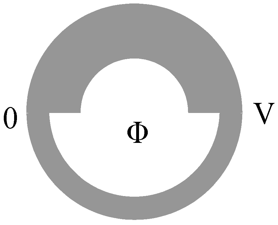
I_Ri plays the role of the viscosity in Section 3, I_Ni plays the role of Brownian hits, and the supercurrent acts as the potential energy. f₁ and f₂ are periodic functions of γ_1,2, so that we have a potential with an unlimited number of minima and maxima. If f₁ and f₂ are not proportional to each other, they behave as an asymmetric potential.

We still require a suitable variation of the potential with time. This is provided by the fluctuations, which are spontaneously present in any phase transition. If the temperature is only slightly below the transition temperature, the superconductivity of the loop is sometimes stronger and sometimes weaker than its equilibrium value. Accordingly, I_ci is sometimes large, so that noise is unable to change the value of γ_i beyond a potential barrier, whereas at other times the opposite occurs.

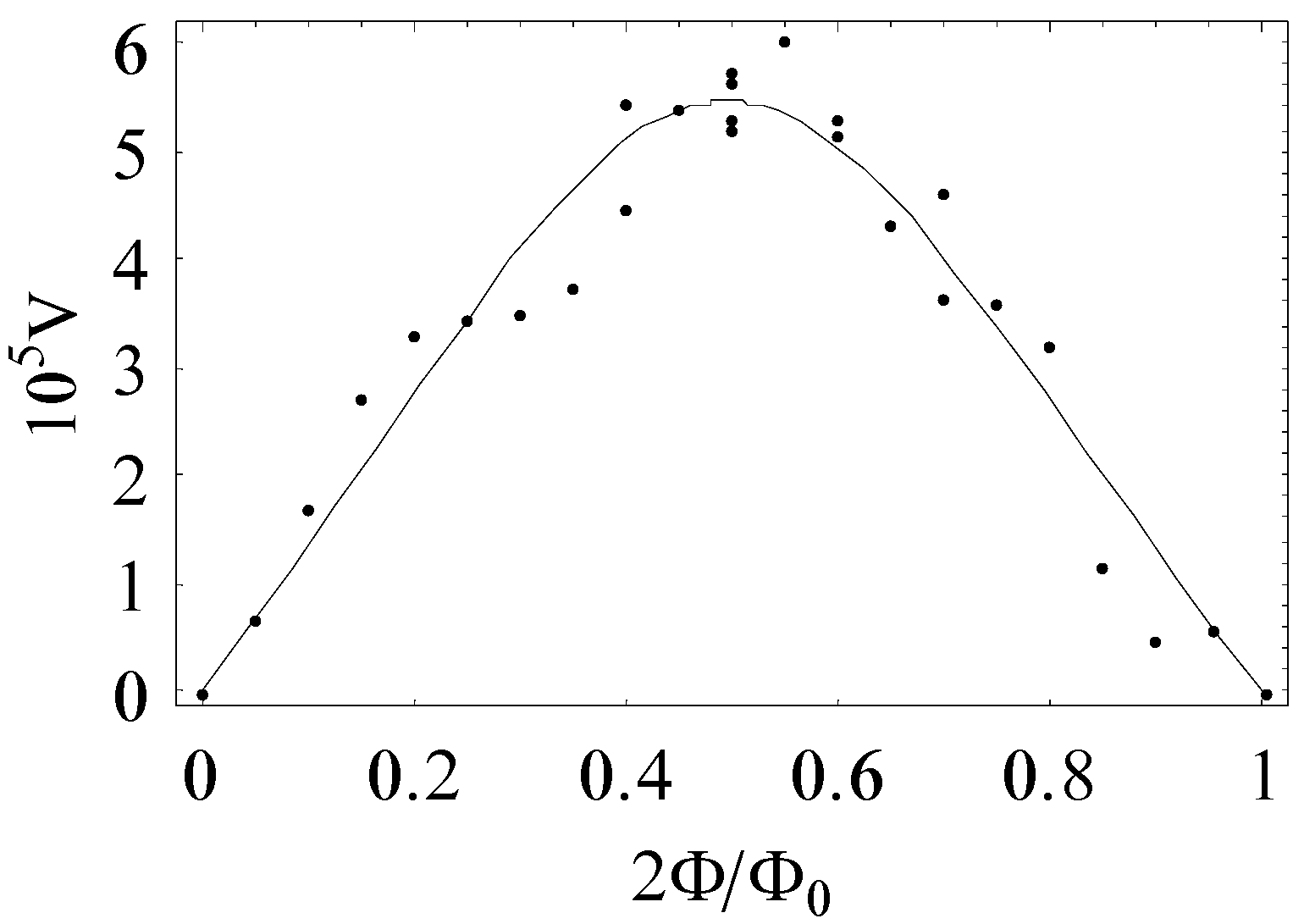
As a result, γ_1,2 drift with time, exactly as the position of the particle in Section 3. According to Josephson's relation, the voltage between the extremes of the segments is proportional to the derivative of γ_i with respect to time. This means that, if γ_i drifts with time, then the average dc voltage doesn't vanish. Figure 4 shows the dc voltage (in normalized units), calculated in Ref. [8] for some particular set of parameters.

Clearly, a dc voltage can be used to perform work. But contrary to the previous section, this time the potential barriers were not raised and withdrawn by an external agent; they spontaneously occurred as a consequence of equilibrium fluctuations. Therefore, as far as I can presently see, this result is in disagreement with the laws of thermodynamics.

The dc voltage between the extremes of the segments of an asymmetric loop has been measured by the Chernogolovka group [9]. The voltage does show up, and does exhibit the expected dependence on the magnetic flux. However, skeptics may still claim that this voltage is induced by ac currents in the region. The same group performed an experiment in which ac currents were intentionally driven through the loop [10]. The dependence of the voltage on the amplitude and on the frequency of the

Figure 4. Voltage between the extremes of the segments of the superconducting loop. The voltage is an odd function of the magnetic flux Φ, and is periodic with period Φ₀, where Φ₀ = 2.07×10^-15 Tm² is the quantum of flux.

Figure 4. Voltage between the extremes of the segments of the superconducting loop. The voltage is an odd function of the magnetic flux Φ, and is periodic with period Φ₀, where Φ₀ = 2.07×10^-15 Tm² is the quantum of flux.

current is the same as that obtained with the Josephson-junctions model, suggesting that, at least qualitatively, this model properly describes the experimental loop.

5. Parrondo's Games

This section is included as an illustration of the fact that a losing trend may be reversed by suitable combinations, not only in physics, but even in mathematics.

Parrondo considers two games, A and B [11]. Game A is simple: in each step there is a probability $\frac{1}{2}-\mathsf{\epsilon }$ of winning 1 euro, and a probability $\frac{1}{2}+\mathsf{\epsilon }$ of losing 1 euro. Clearly, this is a losing game for ε > 0. Game B is more sophisticated: if the number of euros you have left is divisible by 3, then the probability of winning is $\frac{1}{10}-\mathsf{\epsilon }$; if it is not, then the probability of winning is $\frac{3}{4}-\mathsf{\epsilon }$.

Naively, one could think that the probability of having a number divisible by 3 is $\frac{1}{3}$. If this were the case, B would be a winning game for small values of ε . But in order to determine this probability we have to follow the Markovian history of how euros are won or lost. The result is that the probability for divisibility by 3 is $\frac{5}{13}-\frac{440}{2197}\mathsf{\epsilon }$, which is greater than $\frac{1}{3}$. From here it follows that B is a losing game for every ε ∈ (0,0.1).

However, if the losing games A and B are alternated according to some given sequence, or even if they are switched at random, the combination of both can be a winning game for small values of ε.

With a wild imagination, we may now inquire what game B and our superconducting loop have in common. Although B is a losing game, it contains the seeds for winning, because that would be the trend if the number of euros possessed by the player could be treated as a random integer. Therefore, B can become a winning game if this number is randomized by appropriate use of game A. Similarly, our superconducting ring has seeds of order (what Nikulov called a "quantum force" [12]): whenever it becomes superconducting it has to create a persistent current, and whenever it switches to the normal state this current has to be dissipated.

References and Notes

- Hobson, A. Concepts in Statistical Mechanics; Gordon and Breach: NY, 1971. [Google Scholar] Berger, J. The fight against the second law of thermodynamics. Physics Essays 1994, 7, 281–296, (Reprint requests at http://brd4.ort.org.il/~jorge/fight.htm). [Google Scholar] Smith, J.D.H. Some Observations on the Concepts of Information-Theoretic Entropy and Randomness. Entropy 2001, 3, 1–11, (http://www.mdpi.org/entropy/htm/e3010001.htm). [Google Scholar]
- Smoluchowski, M. Experimentell nachweisbare der ublichen thermodynamik widersprechende Molekularphanomene. Phys. Z. 1912, 13, 1069–1080. [Google Scholar] Smoluchowski, M. Vortgage uber die Kinetische Theorie der Materie und der Elektrizitat; Planck, M., Ed.; Taubner und Leipzig: Berlin, 1914; pp. 89–121. [Google Scholar]
- Skordos, P.A.; Zurek, W.H. Maxwell's demon, rectifiers, and the second law: Computer simulation of Smoluchowski's trapdoor. Am. J. Phys. 1992, 60, 876–882. [Google Scholar] [CrossRef]
- Berger, J. Kinetic illustration for thermalization. Am. J. Phys. 1988, 56, 923–928. [Google Scholar] [CrossRef]
- (a)Astumian, R.D.; Hänggi, P. Brownian Motors. Physics Today, November 2002; 33–39, (http://www.aip.org/web2/aiphome/pt/vol-55/iss-11/p33.shtml). [Google Scholar] Astumian, R.D. Making molecules into motors. Sci. Am. 2001, 57–64. [Google Scholar] Astumian, R.D. Thermodynamics and kinetics of a Brownian motor. Science 1977, 276, 917–922. [Google Scholar] [CrossRef] Rousselet, J.; Salome, L.; Adjari, A.; Prost, J. Directional motion of Brownian particles induced by a periodic asymmetric potential. Nature 1994, 370, 446–448. [Google Scholar] [CrossRef] [PubMed]
- http://www.umbrars.com/sr/. Benzi, R.; Sutera, A.; Vulpiani, A. The Mechanism of Stochastic Resonance. J. Phys. A 1981, 14, L453–L457. [Google Scholar] [CrossRef] Wiesenfeld, K.; Moss, F. Stochastic resonance and the benefits of noise: from ice ages to crayfish and SQUIDs. Nature 1995, 373, 33–36. [Google Scholar] [CrossRef] [PubMed]Gammaitoni, L.; Hänggi, P.; Jung, P.; Marchesoni, F. Stochastic Resonance. Rev. Mod. Phys. 1998, 70, 223–287. [Google Scholar] [CrossRef]
- This subject is discussed in many textbooks in superconductivity, e.g. Tinkham, M. Introduction to Superconductivity; McGraw-Hill: NY, 1996. [Google Scholar]
- Berger, J. Noise rectification by superconducting loop with two weak links. Submitted. The first version of this article was posted in http://arxiv.org/abs/cond-mat/0305130.
- Dubonos, S.V.; Kuznetsov, V.I.; Nikulov, A.V. Observation of dc voltage on segments of an inhomogeneous superconducting loop. http://arxiv.org/abs/physics/0105059.
- Dubonos, S.V.; Kuznetsov, V.I.; Zhilyaev, I.N.; Nikulov, A.V.; Firsov, A.A. Induction of dc voltage, proportional to the persistent current, by external ac current on system of inhomogeneous superconducting loops. Zh. Eksp. Teor. Fiz. Pis'ma Red 2003, 77, 439–444, Translated in JETP Lett. 2003, 77, 371-375. (http://arxiv.org/abs/cond-mat/0303538). [Google Scholar]
- http://seneca.fis.ucm.es/parr/GAMES/
- Nikulov, A.V. Quantum force in a superconductor. Phys. Rev. B 2001, 64, 012505, (http://link.aps.org/abstract/PRB/v64/e012505). [Google Scholar]
© 2004 by MDPI (http://www.mdpi.org). Reproduction for noncommercial purposes permitted.
Share and Cite
MDPI and ACS Style
Berger, J. From Randomness to Order. Entropy 2004, 6, 68-75. https://doi.org/10.3390/e6010068
AMA Style
Berger J. From Randomness to Order. Entropy. 2004; 6(1):68-75. https://doi.org/10.3390/e6010068
Chicago/Turabian StyleBerger, Jorge. 2004. "From Randomness to Order" Entropy 6, no. 1: 68-75. https://doi.org/10.3390/e6010068