Langevin approach to the Porto system

Institute of Physics of Charles University, Faculty of Mathematics and Physics, Ke Karlovu 5, CZ-121 16 Prague 2, Czech Republic
*
Author to whom correspondence should be addressed.
Entropy 2004, 6(1), 57-67; https://doi.org/10.3390/e6010057
Submission received: 24 June 2003
/
Accepted: 15 December 2003
/
Published: 12 March 2004
(This article belongs to the Special Issue Quantum Limits to the Second Law of Thermodynamics)
Abstract
:M. Porto (Phys. Rev. E 63 (2001) 030102) suggested a system consisting of Coulomb interacting particles, forming a linear track and a rotor, and working as a molecular motor. Newton equations with damping for the rotor coordinate on the track x, with a prescribed time-dependence of the rotor angle Θ, indicated unidirectional motion of the rotor. Here, for the same system, the treatment was generalized to nonzero temperatures by including stochastic forces and treating both x and Θ via two coupled Langevin equations. Numerical results are reported for stochastic homogeneous distributions of impact events and Gaussian distributions of stochastic forces acting on both the variables. For specific values of parameters involved, the unidirectional motion of the rotor along the track is confirmed, but with a mechanism that is not necessarily the same as that one by Porto. In an additional weak homogeneous potential field U(x) =const·x acting against the motion, the unidirectional motion persists. Then the rotor accumulates potential energy at the cost of thermal stochastic forces from the bath.
1 Introduction
There are many constructions of so called ratchet systems devised to turn stochastic perturbations or noise acting on classical or quantum systems into a unidirectional motion. Perhaps the most famous example is the ‘wind-mill’ system analyzed by Feynman [1]. Detailed analysis mostly revealed that such systems could work but in experimental set-ups devised to violate the Second law of thermodynamics, they fail [1,2]. This fully corresponds to results of multiple theoretical analyses.
Surprisingly, the uni-directionality of the motion has recently been found to be determined not only by a type of asymmetry of the (say) ratchet potentials incorporated but rather dynamically [3,4,5]. The activity in this direction resulted into construction of a relatively realistic model consisting of a molecular rotor on a linear track, both consisting of particles interacting by just Coulomb forces [6]. Under a prescribed time-dependence of the rotor angle Θ(t) entering the potential energy of the system, the classical Newton equation for its linear coordinate x along the track yields that the rotor unidirectionally moves along the track. The prescribed time-dependence Θ(t) may also be stochastic what introduces the idea that one can easily convert the system, upon adding a potential U(x) slightly increasing in the direction of the rotor motion, into a machine converting energy of the stochastic influence of the bath, that might be of thermal origin, into a mechanical potential one. This would mean so called perpetuum mobile of the second kind and a violation of the Second law of thermodynamics.
Porto explicitly refuses this possibility as far as his calculations were concerned - see a note in this respect on page 3 of [6]. Our more general calculation below, however, confirms the above conjecture. Here, we should like to add that this fact is by no means objection against the Porto system and its analysis using the classical Newton equations. Instead, our treatment rather generalizes that one of [6]. First, one can easily justify adding stochastic forces to the Newton equations, converting them into the Langevin ones. In this respect, our calculations below provide a proper extension of those by Porto [6] to finite temperatures. The Langevin equations have well understood quantum counterparts in the Mori or Tokuyama-Mori identities [7,8,9] what makes the calculations even more relevant. Second, the rotor angle Θ has not been here ascribed any specific time-dependence like in [6] but has been assumed to change according to another Langevin equation with the same temperature entering the stochastic force correlations functions; this is rather more physical. In fact, one should not be very much surprised by the challenge to the Second law provided by this amended treatment of the Porto model generalized to finite temperatures. The reason is twofold:
- Second, the present model and its present treatment, though they are perhaps more realistic than often in similar situations, are still just theoretical and their relation to Nature may be not as obvious as it might seem at the first sight.
2 Formulation of the problem
In contrast to the Porto study, we impose no prescribed time-dependence of the Θ(t) variable but describe both the linear coordinate x(t) and the Θ(t) angle as two generalized coordinates describing the rotor (its position as well as the rotation) with their time-dependence determined by a pair of the corresponding coupled Langevin equations. This method supersedes and definitely surmounts the Newton equations used by Porto, in at least the sense that
![Entropy 06 00057 i001]() Here m, J , η and κ are the rotor mass, its moment of inertia, and the linear and angle friction constants. As for the stochastic forces Γx(t) and ΓΘ(t), they should fulfil standard equations
Here m, J , η and κ are the rotor mass, its moment of inertia, and the linear and angle friction constants. As for the stochastic forces Γx(t) and ΓΘ(t), they should fulfil standard equations
![Entropy 06 00057 i002]() ensuring, in absence of the potential Φ(x, Θ), that the asymptotic mean squared velocities
ensuring, in absence of the potential Φ(x, Θ), that the asymptotic mean squared velocities ![Entropy 06 00057 i016]() and
and ![Entropy 06 00057 i017]() fulfil the equipartition theorem with temperature TK. Here
fulfil the equipartition theorem with temperature TK. Here ![Entropy 06 00057 i018]() designates the en-semble average. The stochastic forces are here represented as
designates the en-semble average. The stochastic forces are here represented as
![Entropy 06 00057 i003]() where
where ![Entropy 06 00057 i019]() and
and ![Entropy 06 00057 i020]() are statistically independent times of impact events. Times between two such succeeding impacts are exponentially distributed
are statistically independent times of impact events. Times between two such succeeding impacts are exponentially distributed
![Entropy 06 00057 i004]() (
( ![Entropy 06 00057 i021]() and
and ![Entropy 06 00057 i022]() being the mean waiting times) while distributions
being the mean waiting times) while distributions ![Entropy 06 00057 i023]() and
and ![Entropy 06 00057 i024]() of (also stochastic and statistically independent) impact ‘forces’
of (also stochastic and statistically independent) impact ‘forces’ ![Entropy 06 00057 i025]() and
and ![Entropy 06 00057 i026]() are, on grounds of physical arguments, assumed Gaussian. For (2) to be satisfied, these distributions should read
are, on grounds of physical arguments, assumed Gaussian. For (2) to be satisfied, these distributions should read
![Entropy 06 00057 i005]()
- the Θ(t) variable has its time-dependence determined also from a dynamic equation, and
- this approach respects existing connections between dissipation (friction) incorporated and by its effect decisive in the Porto model, and properties of the stochastic forces on the right hand side of the Langevin equations that were completely ignored in [6].


 and
and  fulfil the equipartition theorem with temperature TK. Here
  designates the en-semble average. The stochastic forces are here represented as

 and
and  are statistically independent times of impact events. Times between two such succeeding impacts are exponentially distributed

 and
and  being the mean waiting times) while distributions
  and
and  of (also stochastic and statistically independent) impact ‘forces’
  and
and  are, on grounds of physical arguments, assumed Gaussian. For (2) to be satisfied, these distributions should read

In order to get the model fully defined, on must specify the potential energy ![Entropy 06 00057 i027]() . It is connected with the definition of the system as given by Porto [6]. The track consists of charges q > 0 at
. It is connected with the definition of the system as given by Porto [6]. The track consists of charges q > 0 at ![Entropy 06 00057 i028]() and
and ![Entropy 06 00057 i029]() with n being arbitrary integer. So, the track is neutral, periodic but without inversion symmetry. The rotor has the total mass m and apart from potentially other neutral atoms, it consists of four point charges
with n being arbitrary integer. So, the track is neutral, periodic but without inversion symmetry. The rotor has the total mass m and apart from potentially other neutral atoms, it consists of four point charges ![Entropy 06 00057 i030]() or 2. Designating as above position of the rotor center of mass as x, their positions are
or 2. Designating as above position of the rotor center of mass as x, their positions are ![Entropy 06 00057 i031]() , 0,
, 0, ![Entropy 06 00057 i032]() . The two radii are
. The two radii are ![Entropy 06 00057 i033]() and
and ![Entropy 06 00057 i034]() . The parameter γ,
. The parameter γ, ![Entropy 06 00057 i035]() , determines the ‘gear’ of the Porto molecular motor model. With that, the potential energy
, determines the ‘gear’ of the Porto molecular motor model. With that, the potential energy ![Entropy 06 00057 i036]() of the configuration of the charges reads
of the configuration of the charges reads
![Entropy 06 00057 i006]()
 . It is connected with the definition of the system as given by Porto [6]. The track consists of charges q > 0 at
  and
and  with n being arbitrary integer. So, the track is neutral, periodic but without inversion symmetry. The rotor has the total mass m and apart from potentially other neutral atoms, it consists of four point charges
  or 2. Designating as above position of the rotor center of mass as x, their positions are
  , 0,
, 0,  . The two radii are
  and
and  . The parameter γ,
  , determines the ‘gear’ of the Porto molecular motor model. With that, the potential energy
  of the configuration of the charges reads

Calculation of the potential ![Entropy 06 00057 i036]() requires some care because the individual sums
requires some care because the individual sums ![Entropy 06 00057 i037]() are divergent.
are divergent.
requires some care because the individual sums  are divergent.
3 Numerical treatment
Before numerical treatment, it is useful to reformulate the problem in dimensional units. We introduce dimensionless coordinates and time by
![Entropy 06 00057 i007]() Then (1) reads
Then (1) reads
![Entropy 06 00057 i008]() where
where
![Entropy 06 00057 i009]() Formulae (3) are then replaced by
Formulae (3) are then replaced by
![Entropy 06 00057 i010]() where, instead of (4), we have distributions of the (statistically independent) dimensionless times
where, instead of (4), we have distributions of the (statistically independent) dimensionless times ![Entropy 06 00057 i038]() and
and ![Entropy 06 00057 i039]()
![Entropy 06 00057 i011]() As for the distributions of the (again statistically independent) ‘forces’
As for the distributions of the (again statistically independent) ‘forces’ ![Entropy 06 00057 i040]() and
and ![Entropy 06 00057 i041]() , we have
, we have
![Entropy 06 00057 i015]()


 and
and 

 and
and  , we have


 sec,
sec,  sec, temperature TK = 300 K and J = 10mb2.
4 Numerical solution
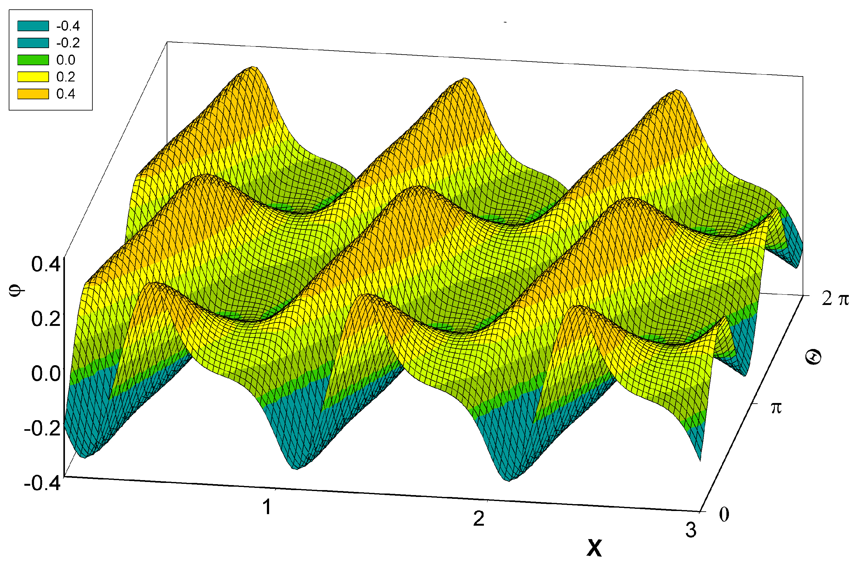
Series for ϕ(X, Θ) in (9) as well as those for its partial derivatives converge very slowly. For numerical solution, however, it is necessary to calculate as accurately as possible. Using extrapolation methods, we were able to calculate all these functions reasonably fast with precision of 12-13 digits at least. Rotor-track potential energy ϕ(X, Θ) is a periodic function in both variables, with period 1 in X (b in x) and π in Θ. Form of this function for the ‘forward gear’ γ = +1 is shown in Fig. 1. Form of the potential profile for γ = −1 (‘reverse gear’) can be deduced from Fig. 1 using identity ϕ(X, Θ, γ = −1) = −ϕ(X, Θ + π/2, γ = +1). The respective positions of extremes for γ = +1 and their values are X = .1179500143638, Θ = .175365440363, ϕ = −.33522791779058053399124 (minimum) and X = .3802499856363, Θ = −.175365440363, ϕ = .33522791779058053399124 (maximum). For γ = −1, the values are X = .3802499856363, Θ = 1.395430886432, ϕ = −.33522791779058053399124 (minimum) and X = .1179500143638, Θ = 1.746161767158, ϕ = .33522791779058053399124 (maximum; all the digits being valid).
Lengths of waiting times between two succeeding impact events were generated from uniformly distributed random numbers r and r′ ∈ (0, 1) using relations WX(T) = − ln(r) and WΘ(T) ![Entropy 06 00057 i049]() . The Gaussian distributed impact forces
. The Gaussian distributed impact forces ![Entropy 06 00057 i050]() and
and ![Entropy 06 00057 i051]() were generated using procedure gasdev from [20].
were generated using procedure gasdev from [20].
 . The Gaussian distributed impact forces
  and
and  were generated using procedure gasdev from [20].
Between any two impact events, set of equations (8) was solved using the Bulirsch-Stoer method (procedure bsstep from [20]), with numerical constants as in (13). Values of constants ![Entropy 06 00057 i044]() and
and ![Entropy 06 00057 i045]() are then .0101 and 127.5, respectively. The ratio
are then .0101 and 127.5, respectively. The ratio ![Entropy 06 00057 i046]() . Initial values of X and Θ were always chosen at minimum points of the potential energy ϕ (see above); initial values of
. Initial values of X and Θ were always chosen at minimum points of the potential energy ϕ (see above); initial values of ![Entropy 06 00057 i047]() and
and ![Entropy 06 00057 i048]() were always chosen as zero.
were always chosen as zero.
 and
and  are then .0101 and 127.5, respectively. The ratio
  . Initial values of X and Θ were always chosen at minimum points of the potential energy ϕ (see above); initial values of
  and
and  were always chosen as zero.
Because of the nonlinearity of (8), one must expect a chaotic behavior (extreme sensitivity to numerical values of initial conditions as well as finite accuracy of the numerical calculations). Fig. 2 and Fig. 3 illustrate the onset of the chaos. For our accuracy 10−13 in integration of the diff rential equations (8) and the above accuracy of calculation of derivatives of ϕ, the chaos starts to appear always at about T = 1200.
5 Results
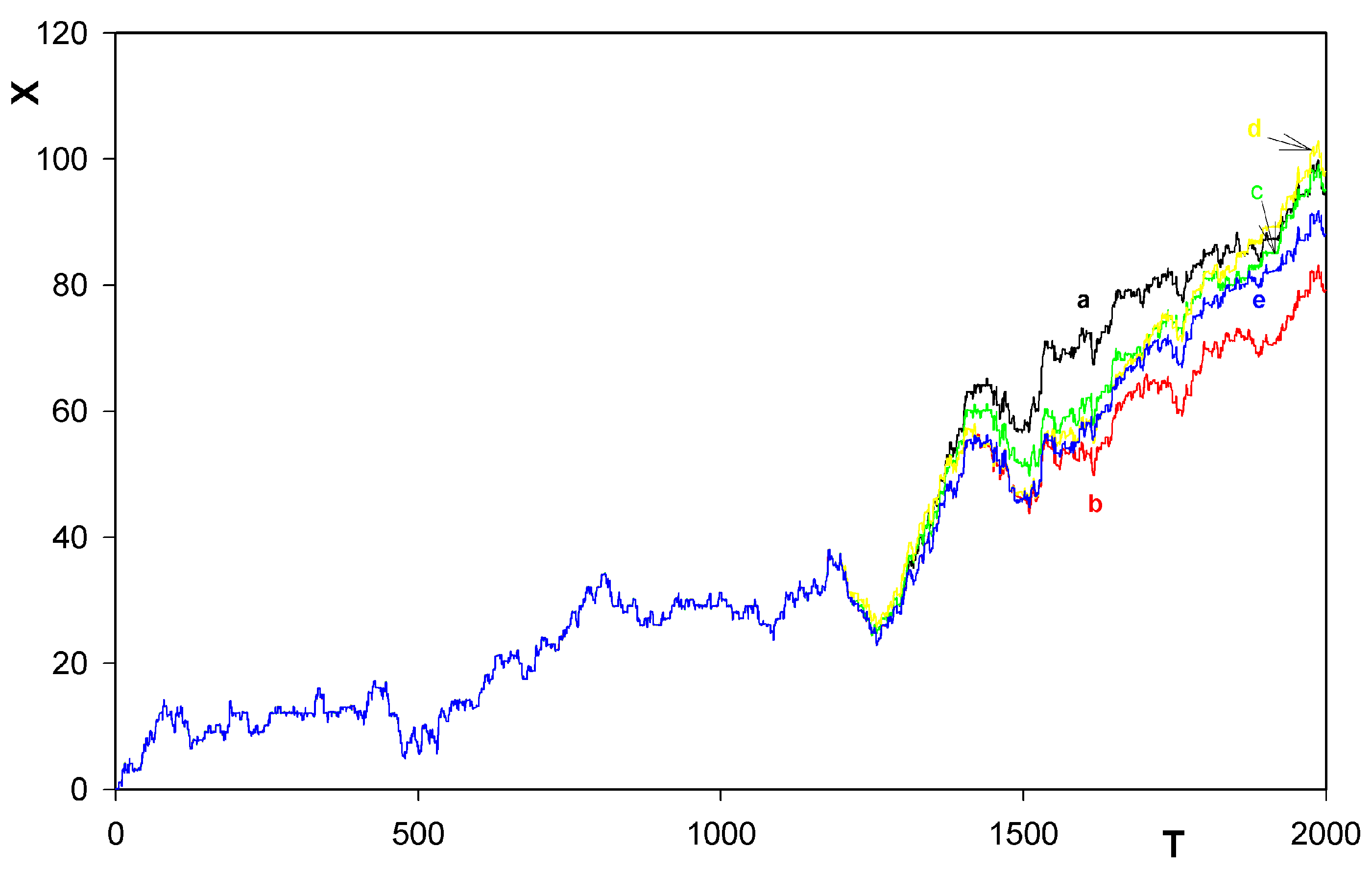
Fig. 4 and Fig. 5 illustrate time-dependence of solution for X(T) for different sequences of the random numbers (i.e. impact events as well as the values of the impact forces) involved. In agreement with Porto’s results, the tendency of behavior of X(T) is to increase (for the ‘forward gear’) and to decrease (for the ‘reverse gear’) with increasing T. One of the curves in Figure 4 in interval (1,1000) provides an exception from the rule. Nevertheless, extending the calculations up to T = 4000, general tendency of final increase was anyhow finally found to appear also here. Because of lack of the random forces in the Porto calculations, no such exceptional behavior could be found by him. Figure 6 shows a new remarkable feature of our calculations. As Porto, in [6], has in fact solved the problem for just X with a prescribed dependence of Θ(T), and because his calculations involved no stochasticity, his only mechanism for the forward and backward motion of the rotor along the track was that one owing to the tendency of X(T) to relax fast, at any time, to a minimum of the potential ϕ(X, Θ) with the prescribed instantaneous value of Θ. Thus, in his case, coordinate X(T) continually moves along valleys of the potential profile being driven by the prescribed time dependence of Θ. Because we have in our case also the stochastic impacts on the coordinate X included, the rotor motion along the track could also be owing to the impact-induced hops of the rotor between two neighboring minima of ϕ, without any essential change of the ‘slow’ variable Θ. (In the whole interval (0,25) in Figure 6, Θ changes by just about 1/27 of a turn.) Fortunately, as Figure 6 shows, direction of the prevailing motion owing to this new mechanism is the same as that one owing to the Θ-induced motion of X(T) by Porto. Thus, the two mechanisms of the rotor motion along the track rather support each other.
The whole beauty of the behavior of the system just reported becomes explicit when we realize that the unidirectional tendency of the rotor motion could survive even when we add a smooth potential acting against the above two mechanisms. In order to make the the situation more clear, we have added, to the potential ϕ(X, Θ) above, a linear potential
![Entropy 06 00057 i014]()

In Figure 7, we can see some results of the simulation. The curves correspond to otherwise exactly the same parameters as in Figure 4. Worth noticing is that even the curve, that virtually corresponded to the backwards motion of the rotor in the limited time-interval investigated, turns now up to describe, like all other curves, motion of the rotor against the homogeneous potential field (14). Thus, because of the periodicity of ϕ(X, Θ), the system starts now to accumulate the potential energy δϕ(X, Θ). The question is what is the source of this acquired potential energy that could be later used in any prescribed way. We can see its only source - this is the above stochastic behavior simulating influence of a real bath on the system. If so, the behavior of course becomes incompatible with the standard thermodynamics. This illustrates how the physics behind, in particular, the Second law of thermodynamics is still little understood.
6 Conclusions
The generalized Porto model introduced above, as defined by the Porto system [6] and the Langevin equations (1) describing its behavior in external stochastic fields modelling influence of the thermal bath, provides a relatively realistic model that makes numerical studies of its time development reasonable. Though the description by the Langevin equations is classical, it should be taken seriously because of existing quantum counterparts of these equations. This makes the basic conclusions obtained relevant. These are, in particular:
- Confirmation, at finite temperatures, that the rotor has a tendency to move along the track in prevailingly one direction only. This tendency was already found, in his simplified treatment corresponding inter alia to zero temperature, by Porto [6].
- Identification of another mechanism (in addition to that one found by Porto himself) also leading the unidirectional motion of the rotor along the train.
- Survival of the behavior even when the motion goes against a weak potential field.
The latter characteristic behavior indicates possible incompatibility of the model and its description via the Langevin equations with principles of the statistical thermodynamics.
7 Acknowledgement
This work is a part of the research program MSM113200002 financed by the Ministry of Education of the Czech republic.
References
- Feynman, R. P.; Leighton, R. B.; Sands, M. The Feynman Lectures in Physics (Addison-Wesley, Reading, 1963). Vol. 1. Chapter 46.
- Musser, G. Scientific American 280. No 2. 1999; 13. [Google Scholar]
- Porto, M.; Urbakh, M.; Klafter, J. Phys. Rev. Letters 84. 2000, 6058.
- Porto, M.; Urbakh, M.; Klafter, J. Phys. Rev. Letters 85. 2000, 491.
- Porto, M.; Urbakh, M.; Klafter, J. Acta Physica Polonica B 2001, 32, 295.
- Porto, M. Phys. Rev. E 2001, 63, 030102.
- Mori, H. Progr. Theor. Phys. 1995, 33, 423.
- Tokuyama, M.; Mori, H. Progr. Theor. Phys. 1976, 55, 411.
- Fick, E.; Sauermann, G. The Quantum Statistics of Dynamic Processes. Springer Series in Solid-State Sciences 86, (Springer-Verlag, Berlin - Heidelberg - New York - London - Paris - Tokyo - Hong Kong - Barcelona, 1990.).
- Čápek, V.; Czech. J. Phys. 1997, 47, 845.
- Čápek, V. Phys. Rev. E 1998, 57, 3846.
- Čápek, V.; Bok, J. Physica A 2001, 290, 379.
- Nikulov, A. V. Phys. Rev. B 2001, 64, 012505.
- Čápek, V. Europ. J. Phys. B 2002, 25, 101. [Google Scholar]
- Čápek, V.; Mančal, T. J. Phys. A 2002, 35, 2111.
- Sheehan, D. P. Phys. Plasmas 1995, 2, 1993.
- Nikulov, A. V.; Zhilyaev, I. N. J. Low Temp. Phys. 1998, 112, 227.
- Dubonos, S. V.; Kuznetsov, V. I.; Nikulov, V. http://arxiv.org/abs/physics/0105059.
- Čápek, V.; Sheehan, D. P. Physica A 2002, 304, 461.
- Press, W. H.; Teukolsky, S. A.; Vetterling, W. T.; Flannery, B. P. Numerical Recipes in Fortran; Cambridge University Press: Cambridge (UK), 1992. [Google Scholar]
Figure 1.
Plot of the dimensionless rotor-track potential energy ψ for γ = +1 as a function of X and Θ.
Figure 1.
Plot of the dimensionless rotor-track potential energy ψ for γ = +1 as a function of X and Θ.

Figure 2.
Time dependence of angle Θ as a function of T for γ = +1 and the same values of all the input parameters as specified in the main text. In all three cases, the impact times as well as the random forces were identical. Only in time intervals between any two individual impacts, different integration time steps (1/32, 1/16, 1/10, 1/8 and 1/7 for curves a) to e), respectively) were used. The onset of chaos appears at about T = 1200. At T = 1000, the values of Θ obtained still coincided to 5 digits.
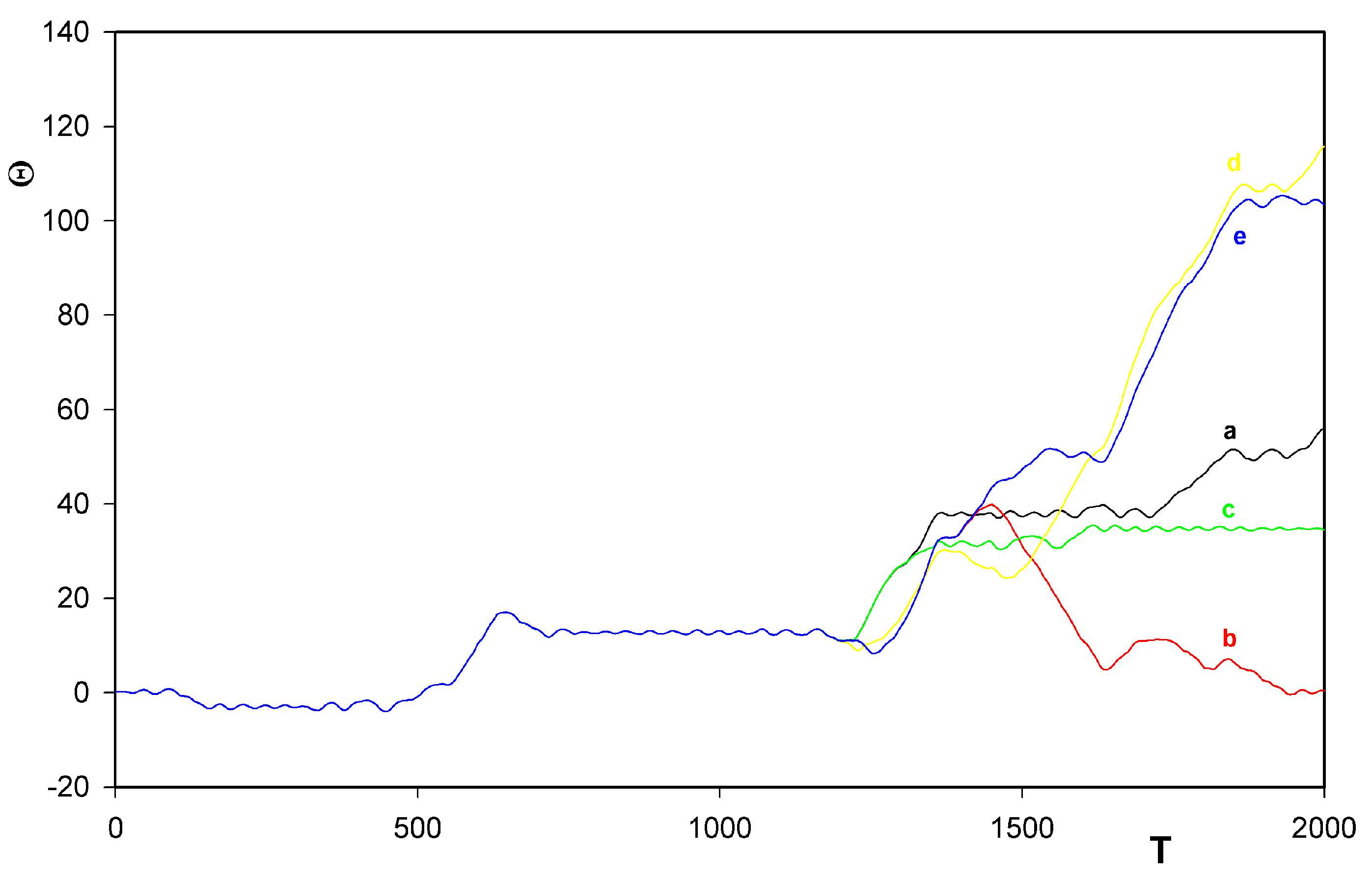
Figure 3.
The same for X as a function of T for the same values of all the input parameters. At T = 1000, the values of X obtained still coincided to 6 digits. Notice that all the curves increase with increasing time.
Figure 3.
The same for X as a function of T for the same values of all the input parameters. At T = 1000, the values of X obtained still coincided to 6 digits. Notice that all the curves increase with increasing time.

Figure 4.
Dependence of X on T for five different sequences of the random numbers involved for the ‘forward gear’ γ = +1.
Figure 4.
Dependence of X on T for five different sequences of the random numbers involved for the ‘forward gear’ γ = +1.
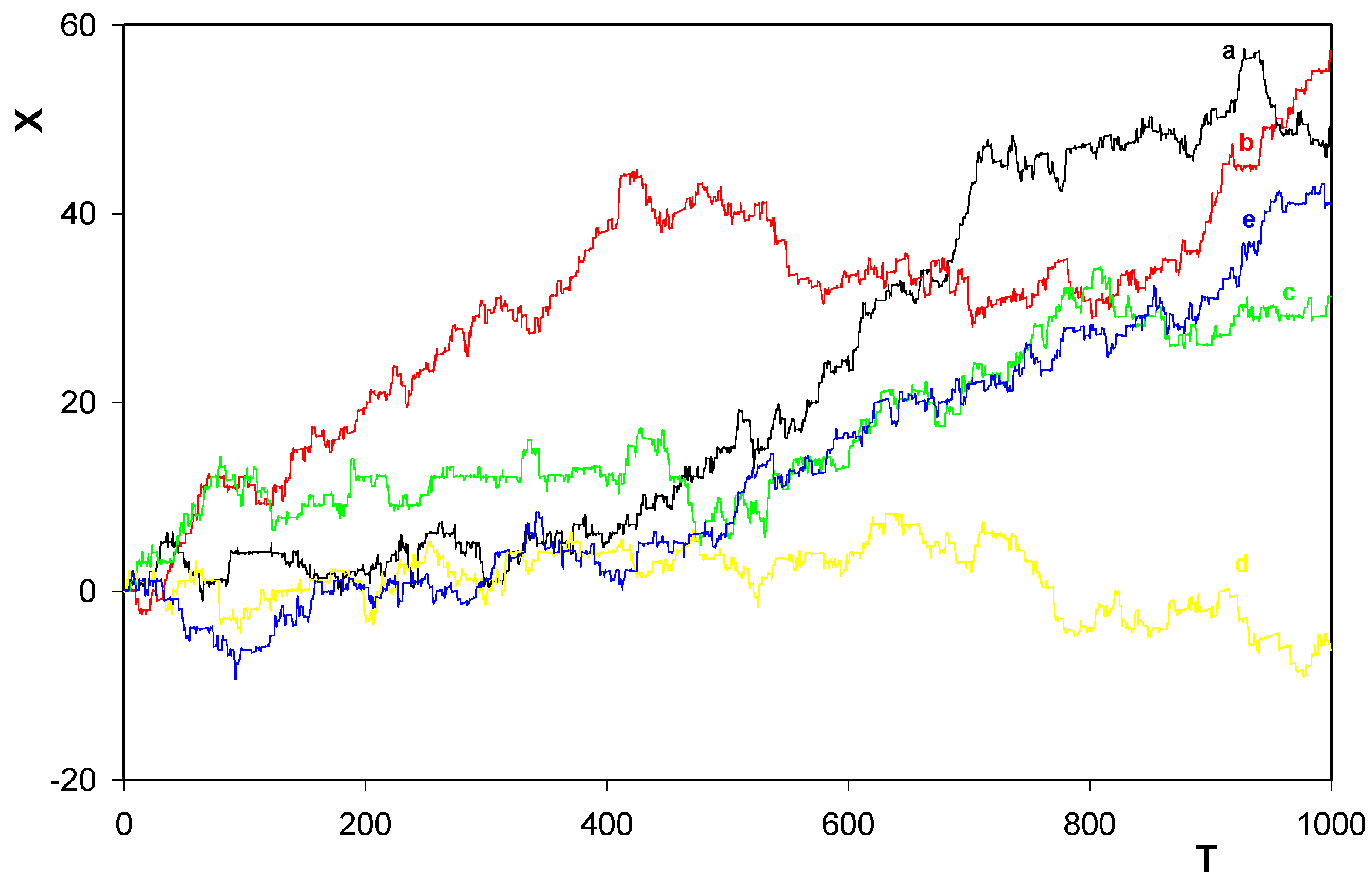
Figure 5.
The same for the ‘reverse gear’ γ = −1. The same sequences of random numbers as in Figure 4 were used.
Figure 5.
The same for the ‘reverse gear’ γ = −1. The same sequences of random numbers as in Figure 4 were used.
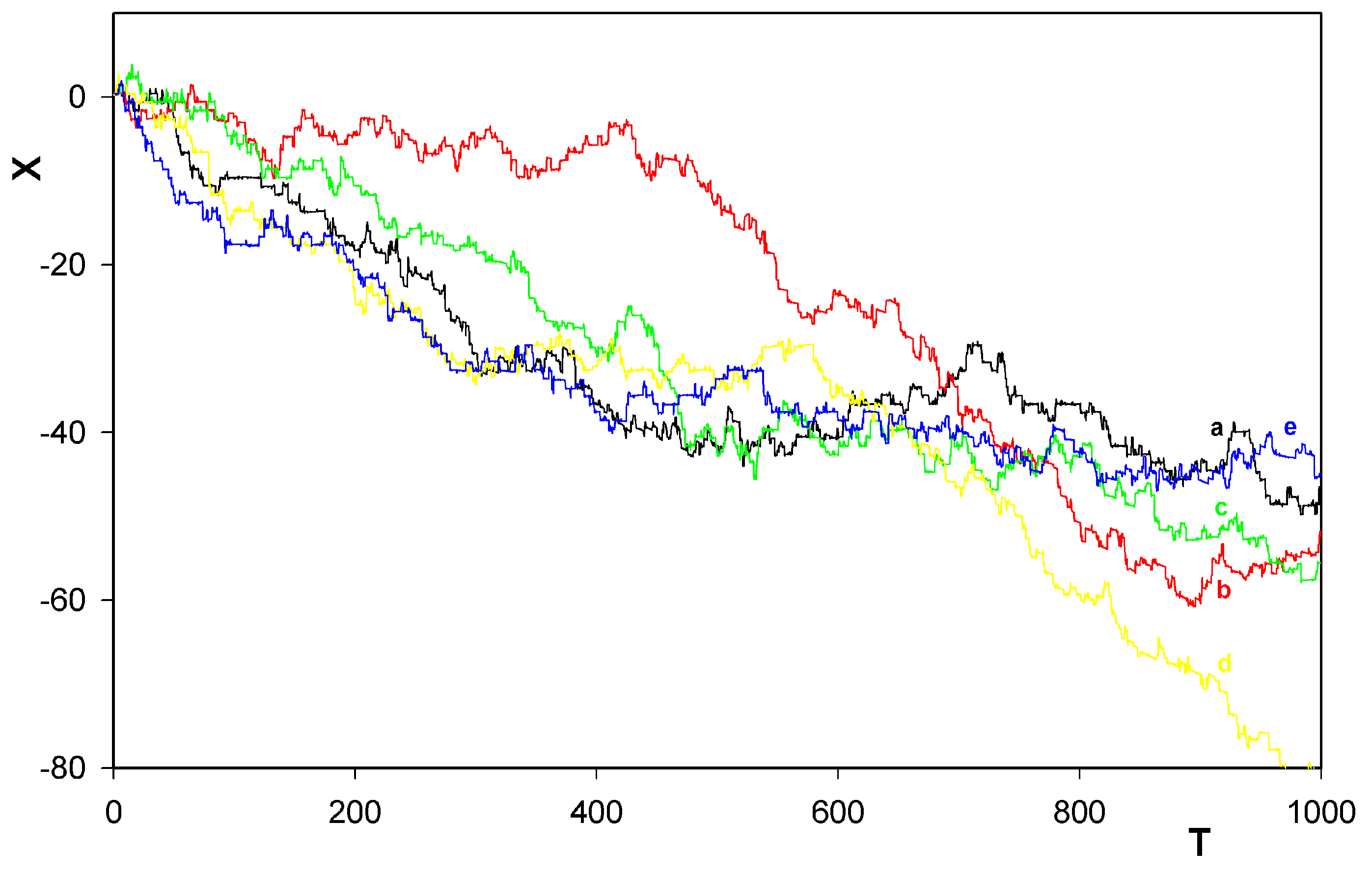
Figure 6.
Details of time-dependence of X(T) (γ = +1) for curve ‘c’ of Figure 4 before the first impact event in Θ occurs. Times T of the first six impacts in X were 4.4506, 5.0489, 5.9216, 9.7589, 9.9581, and 10.7401. The first impact in Θ appears at T = 216.8751. Worth noticing is how the impacts cause, because of the periodicity of ψ, sudden changes of X = x/b (on the vertical axis) by integers.
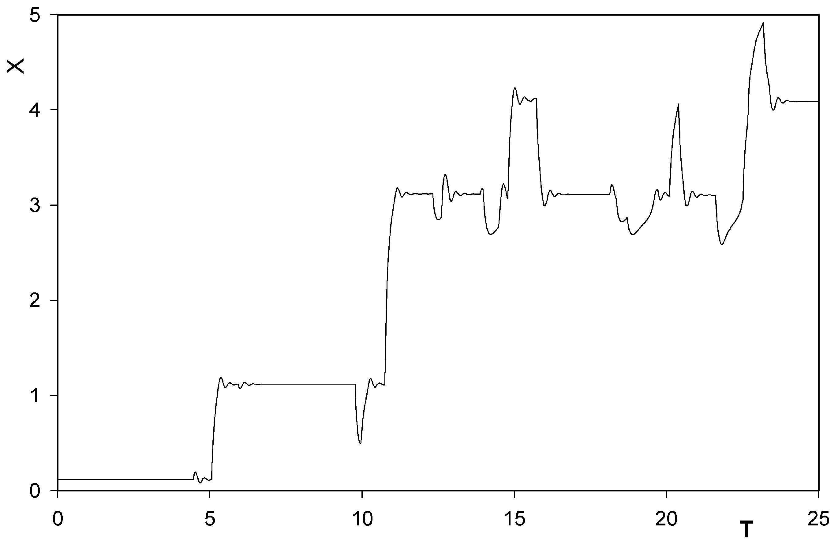
Figure 7.
Dependence of X on T for five different sequences of the random numbers involved for the ‘forward gear’ γ = +1. All the input parameters as well as the random forces were identical as in Figure 4, but with the linear potential c · X, c = 0.01 added to ψ(X, Θ).
Figure 7.
Dependence of X on T for five different sequences of the random numbers involved for the ‘forward gear’ γ = +1. All the input parameters as well as the random forces were identical as in Figure 4, but with the linear potential c · X, c = 0.01 added to ψ(X, Θ).

© 2004 by MDPI (http://www.mdpi.org). Reproduction for noncommercial purposes permitted.
Share and Cite
MDPI and ACS Style
Bok, J.; Cápek, V. Langevin approach to the Porto system. Entropy 2004, 6, 57-67. https://doi.org/10.3390/e6010057
AMA Style
Bok J, Cápek V. Langevin approach to the Porto system. Entropy. 2004; 6(1):57-67. https://doi.org/10.3390/e6010057
Chicago/Turabian StyleBok, Jirí, and Vladislav Cápek. 2004. "Langevin approach to the Porto system" Entropy 6, no. 1: 57-67. https://doi.org/10.3390/e6010057