Entropy Generation in Laminar Fluid Flow through a Circular Pipe

Department of Mechanical Engineering, King Fahd University of Petroleum and Minerals, Dhahran 31261, Saudi Arabia
*
Author to whom correspondence should be addressed.
Entropy 2003, 5(5), 404-416; https://doi.org/10.3390/e5050404
Submission received: 21 November 2002
/
Accepted: 1 June 2003
/
Published: 31 December 2003
(This article belongs to the Special Issue Entropy Generation in Thermal Systems and Processes)
Abstract
:A numerical solution to the entropy generation in a circular pipe is made. Radial and axial variations are considered. Navier-Stokes equations in cylindrical coordinates are used to solve the velocity and temperature fields. Uniform wall heat flux is considered as the thermal boundary condition. The distribution of the entropy generation rate is investigated throughout the volume of the fluid as it flows through the pipe. Engine oil is selected as the working fluid. In addition, water and Freon are used in a parametric study. The total entropy generation rate is calculated by integration over the various cross-sections as well as over the entire volume.
1. Introduction
Second law of thermodynamics states that all real processes are irreversible. Entropy generation is a measure of the amount of irreversibility associated with the real processes. As entropy generation takes place, the quality of energy (i.e. the exergy) decreases [1]. This is a reality in any fluid flow process. In order to preserve the quality of energy in a fluid flow process or at least to reduce the entropy generation, it is important to study the distribution of the entropy generation within the fluid volume.
There have been a number of studies on the entropy generation in fluid flow related problems. Bejan [2,3] showed that the entropy generation for forced convection viscous fluid flow in a channel is due to heat transfer and viscous friction in the fluid. Bejan showed that when the entropy generation is minimized, for the case of heat transfer in a circular tube, a trade-off exists between the components of entropy generation associated with heat transfer end viscosity effects. Bejan [4] also applied the concept of minimum entropy generation to the design of a counter-flow heat exchanger. He showed that an optimum flow path length would be possible.
Viscous dissipation and flow work in ducts have been studied by many investigators (e.g. [5,6,7,8]). Brinkman [6] and Ou and Cheng [8] studied the effect of viscous dissipation on thermal entrance heat transfer in pipe flows with uniform wall temperature. The effect of viscous dissipation on the thermal entrance heat transfer in ducts with constant wall heat flux has been investigated by Brinkman [6] and Ou and Cheng [7] with the assumption of constant viscosity and fully developed velocity profiles. Effectiveness and design of heat exchangers have also been studied extensively in the literature [9,10,11]. Application of the second law analysis for some steady flow devices can be found in references [12,13,14].
Nag and Kumar [15] studied the second law optimization for convective heat transfer through duct at constant heat flux boundary condition. Sahin [16] studied the second law analysis of viscous fluid in circular duct with isothermal boundary condition. Later, he [17] presented the effect of variable viscosity on entropy generation rate for constant heat flux boundary condition for circular duct. The fluid flow considered in all of these studies is one-dimensional. Distribution of entropy generation in the volume of fluid becomes important to determine the regions of possible concentration of entropy generation. Thus, the main objective of the present study is to investigate the entropy generation in a circular pipe as a two dimensional problem. Developing flow with uniform wall heat flux boundary condition is considered. Engine oil is chosen as the working fluid. A parametric study is also made using water and Freon to observe the effect of the Reynolds number. Variation of the entropy generation rate throughout the fluid volume is studied.
2. Analysis
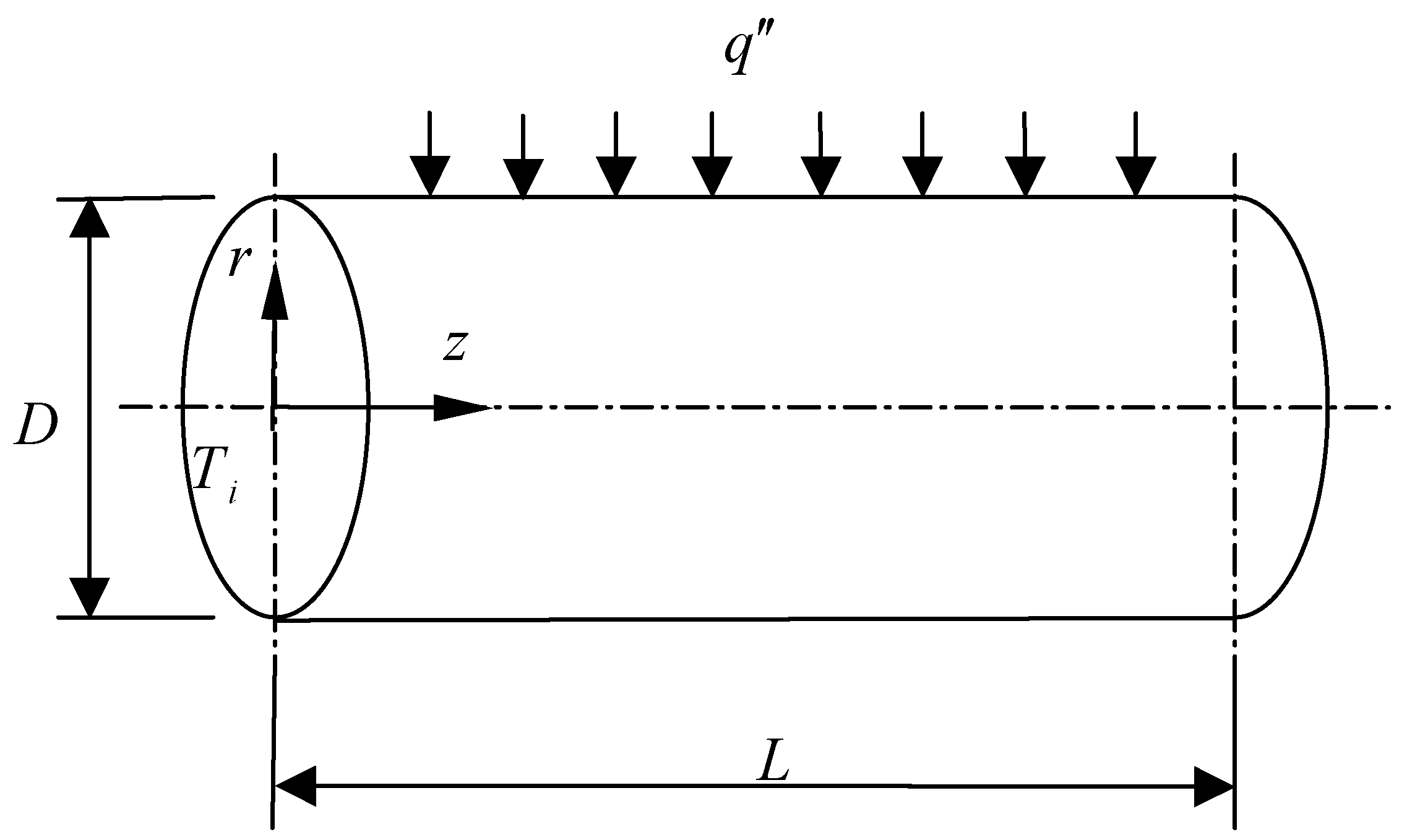
Consider a circular pipe of diameter D and length L, through which a viscous fluid is transported, as shown in Figure 1. The thickness of the pipe is neglected and the thermal boundary condition on the surface of the pipe is assumed to be uniform heat flux q”. Fluid enters the pipe with uniform axial velocity vz0 and uniform temperature Ti. Both hydrodynamic and thermal boundary layers start developing. The purpose is to study the volumetric entropy generation rate distribution throughout the fluid in the pipe. This requires solution of velocity and temperature fields in the fluid. The governing equations and the boundary conditions for this steady problem with constant thermophysical properties are as follows [18]:
Continuity:
Momentum:
Energy:
Entropy Generation rate [3]:
where the dissipation function is given by
The first term in equation (5) represents the entropy generation due to heat conduction in the radial and axial directions. The last term, on the other hand, accounts for the fluid friction contribution to the entropy generation. Bejan number that is the ratio of the entropy generation due to the heat transfer to the total entropy generation is given by [19]
The flow boundary conditions used are as follows:
- vr= 0, vz = 0 at the wall
- vr = 0, vz = vz 0 at the inlet where vz0 is a constant value.
- , at the outlet section providing a fully developed flow condition.
The thermal boundary conditions assume the following:
- A constant heat flux is imposed at the wall q” = q0 where q0 is a constant.
- T = Ti at the inlet section of the pipe where Ti is constant.
- at the outlet. This condition may not be fully valid as the thermal boundary layer is still developing, but it is necessary to limit the computational domain. This condition introduces some error in the last three nodes of the calculations which have been accounted for in the post-processing of the results.
3. Results and Discussion
The solution of the problem has been carried out by FLUENT software. The working fluid considered is engine oil whose thermophysical properties are given in Table 1. In addition, water and Freon are used for a parametric study.
The CFD software employed uses the finite volume technique which is well documented in the literature [20]. The computational domain included half the pipe of D=2.5cm diameter and a length L=1 m. The grid used was constructed out of a structured mesh with 30 nodes in the radial direction and 400 nodes in longitudinal direction. To capture the boundary layer, smaller spacing was put close to the wall with a successive ration of 1.04 away from the wall.
A grid refinement study was conducted to check the validity of numerical study. The results of the two final grids are summarized in Table 2. The results indicate that all values compared are less then 1% difference indicating the 30x400 grid is enough to obtain good results. As indicated by the axial velocity profiles, both grids predict the entry length at about 0.012 which agrees very well with the correlated equation of 0.05 ReD that gives 0.011 in this case.
The solution was run on a Pentium workstation with double presision option and was converged until the residuals were smaller than 10-7 for the continuity and momentum equtions and smaller than 10-10 in the energy equation.
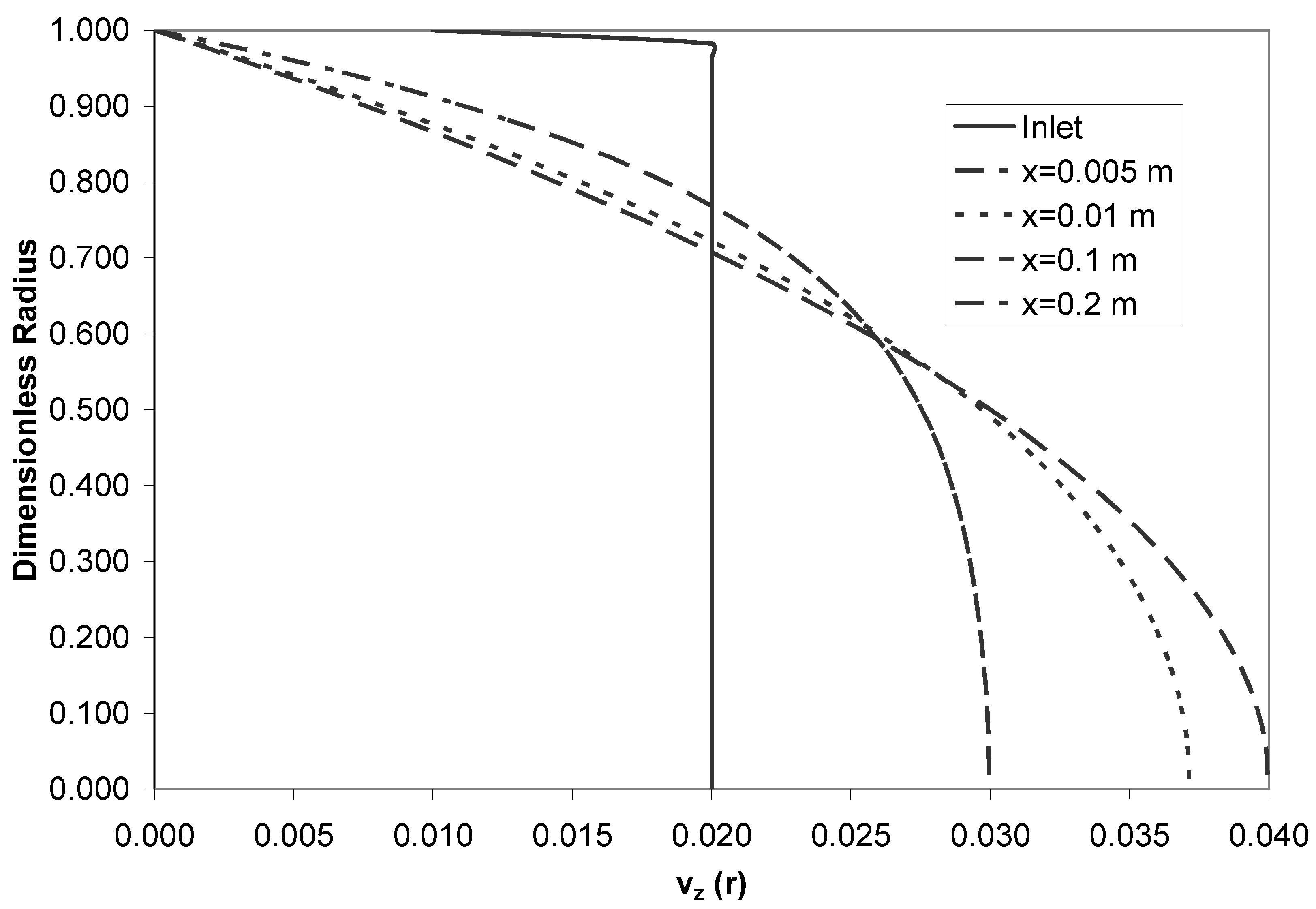
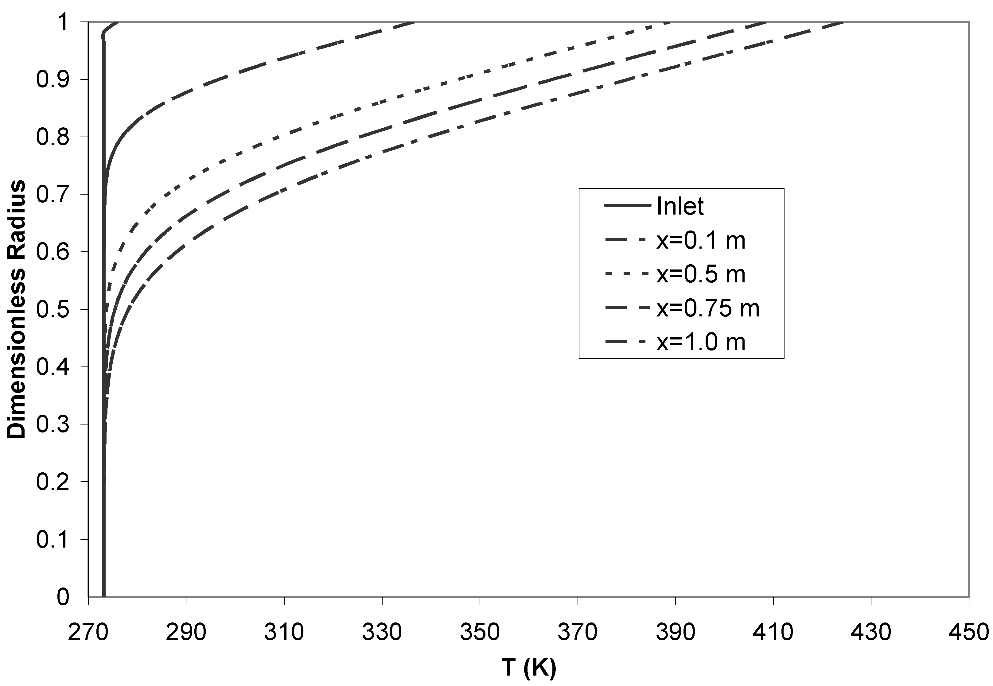
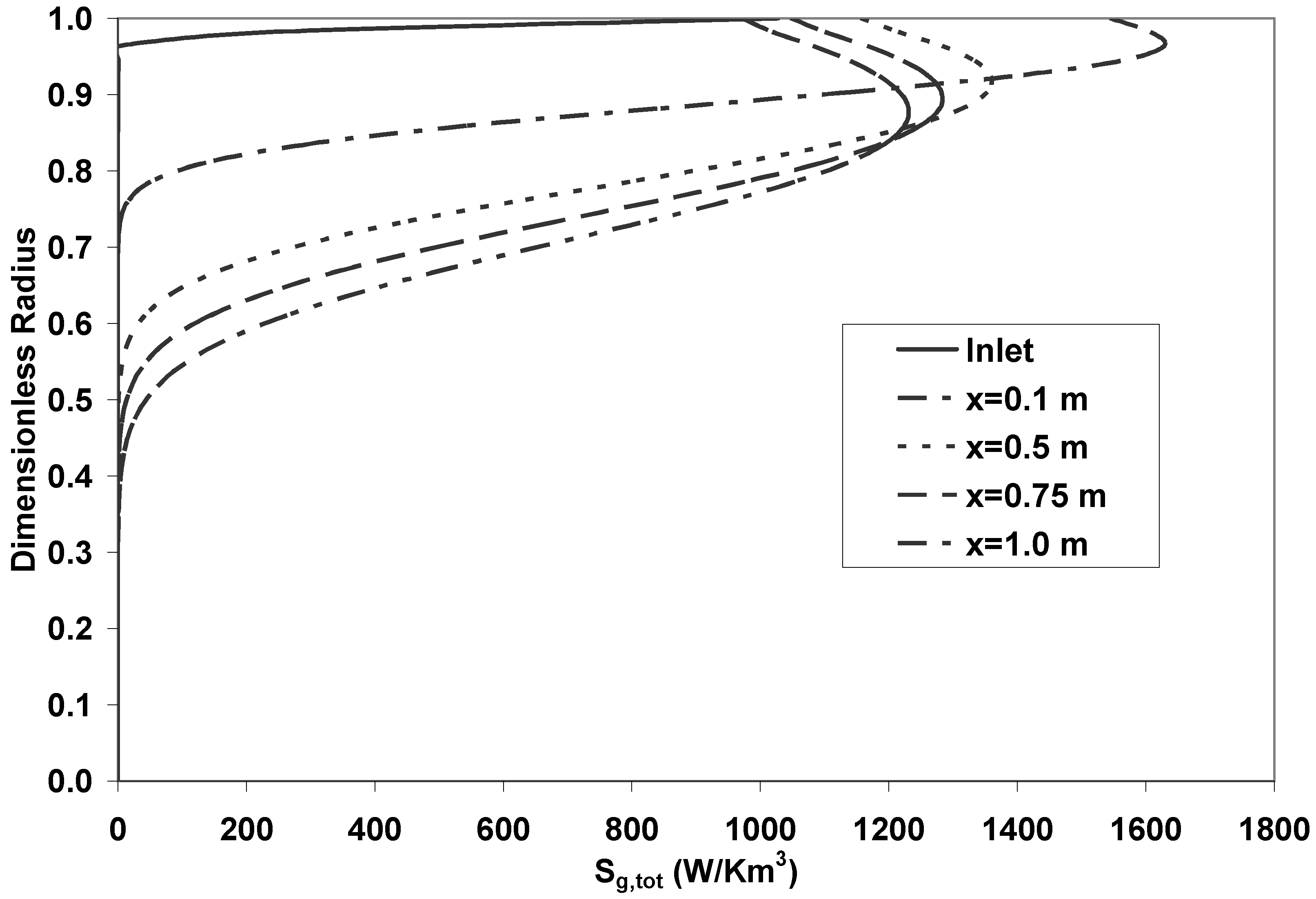
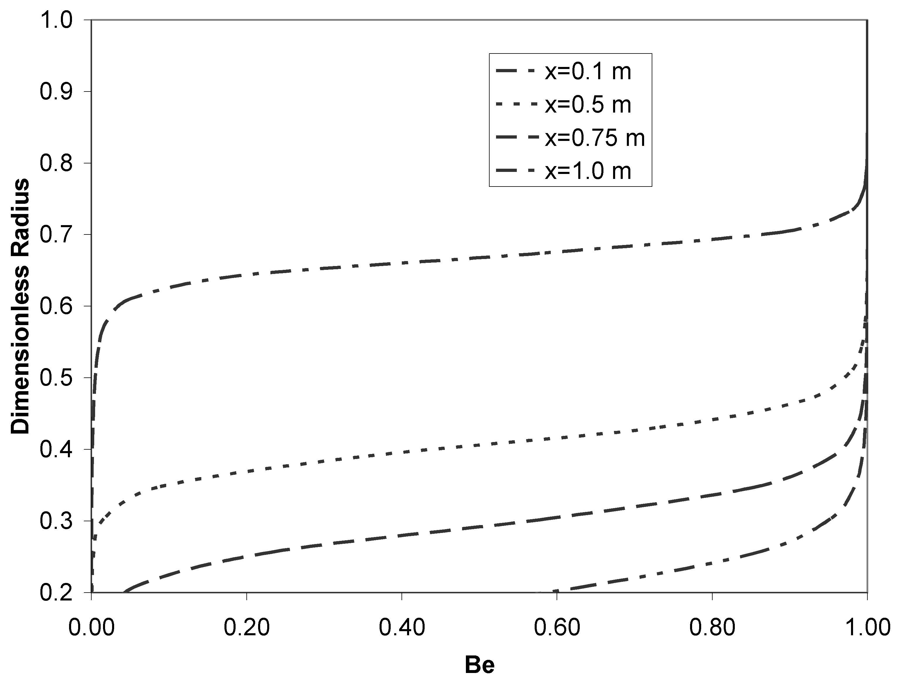
Figure 2 shows the radial velocity profiles at various downstream axial locations starting from the inlet. At the inlet uniform velocity of 0.02 m/s is considered. The development of the hydrodynamic boundary layer has been fast. Fully developed flow has been reached within about 20 cm from the inlet. Since the thermophysical properties are assumed to be constant, the fully developed velocity profile is found to be parabolic with a maximum of 0.04 m/s, i.e. twice as the average velocity that is equal to the uniform inlet velocity. Figure 3 shows the radial temperature profiles at different axial locations along the pipe. The Pr number is calculated to be Pr = µCp/k = 13395, thus the thermal boundary layer is not expected to develop fully within the length of the pipe considered that is 1 m. The temperature profiles therefore change continuously starting from the uniform distribution at the inlet through the pipe and until the exit. The wall boundary condition is uniform heat flux. Therefore, the wall temperature rises continuously and heat penetration takes place in the radial direction. Although full penetration of heat up to the centerline has not been reached, our concern was in fact to study only the entry region of the pipe and analyze the entropy generation in this region. Figure 4 shows the radial entropy generation rate profiles at different axial locations. Near the entrance, the entropy generation is confined in a narrow region next to the wall. As the thermal penetration takes place along the pipe the entropy generation region widens but the peak value of entropy generation rate decreases. The Bejan number that is defined as the fraction of the thermal component of the entropy generation to the overall (thermal and viscous components together) entropy generation is shown in Figure 5. The Bejan number is small close to the centerline but quickly reaches the value of 1 along the radial direction. This indicates that the major component for the entropy generation rate is the thermal component.
Axial variations of temperature and entropy generation rate are given in Figure 6 and Figure 7, respectively. Temperature of the fluid near the wall rises continuously. The centerline temperature remained unchanged, because heat penetration has not reached the centerline for the pipe of length 1 m. Entropy generation rate near the wall increases sharply and then decreases along the pipe as shown in Figure 7. Along the centerline the entropy generation rate is zero as the temperature gradient is zero and the velocity gradients are either very small or zero. Integrated values of entropy generation rate over the cross-section of the pipe for various axial locations are given in Table 3 for three different fluids. In general, a gradual increase in the entropy generation rate over the cross-section is observed. This is due to the widening of the thermal boundary layer and increase of temperature gradients as the fluid is heated along the pipe.
Overall integrated value of the entropy generation rate over the volume for engine oil is calculated to be 0.2537 W/K. At this point, a thermodynamic analysis may be useful in order to verify the accuracy of the analysis and the numerical solution.
The total heat transfer rate to the pipe is
Thus the exit bulk temperature becomes
where and .
Using the thermophysical properties given in Table 1, the exit bulk temperature is calculated to be 297.5 K. The total entropy generation rate is
In this equation Tw is an unknown. Therefore a precise calculation for the entropy generation rate is not possible. Looking at the numerical solution for the wall temperature variation in Figure 6, the average wall temperature appears to be around 370 K. When this value of wall temperature is used the overall entropy generation rate is calculated to be 0.3157 W/K. This indicated a 20% deviation (underestimation) of the numerical solution which was 0.2537 W/K. On the other hand, if the average wall temperature is taken to be 350 K, the two solutions match almost identically. Based on the assumptions made for the thermophysical properties and the boundary conditions the numerical solution of the wall temperature is not expected to represent the real situation accurately. Therefore the real solution would be expected to be somewhere in between, i.e. the average wall temperature should be between 350 and 370 K and the overall entropy generation rate is expected to be between 0.2537 and 0.3157 W/K.
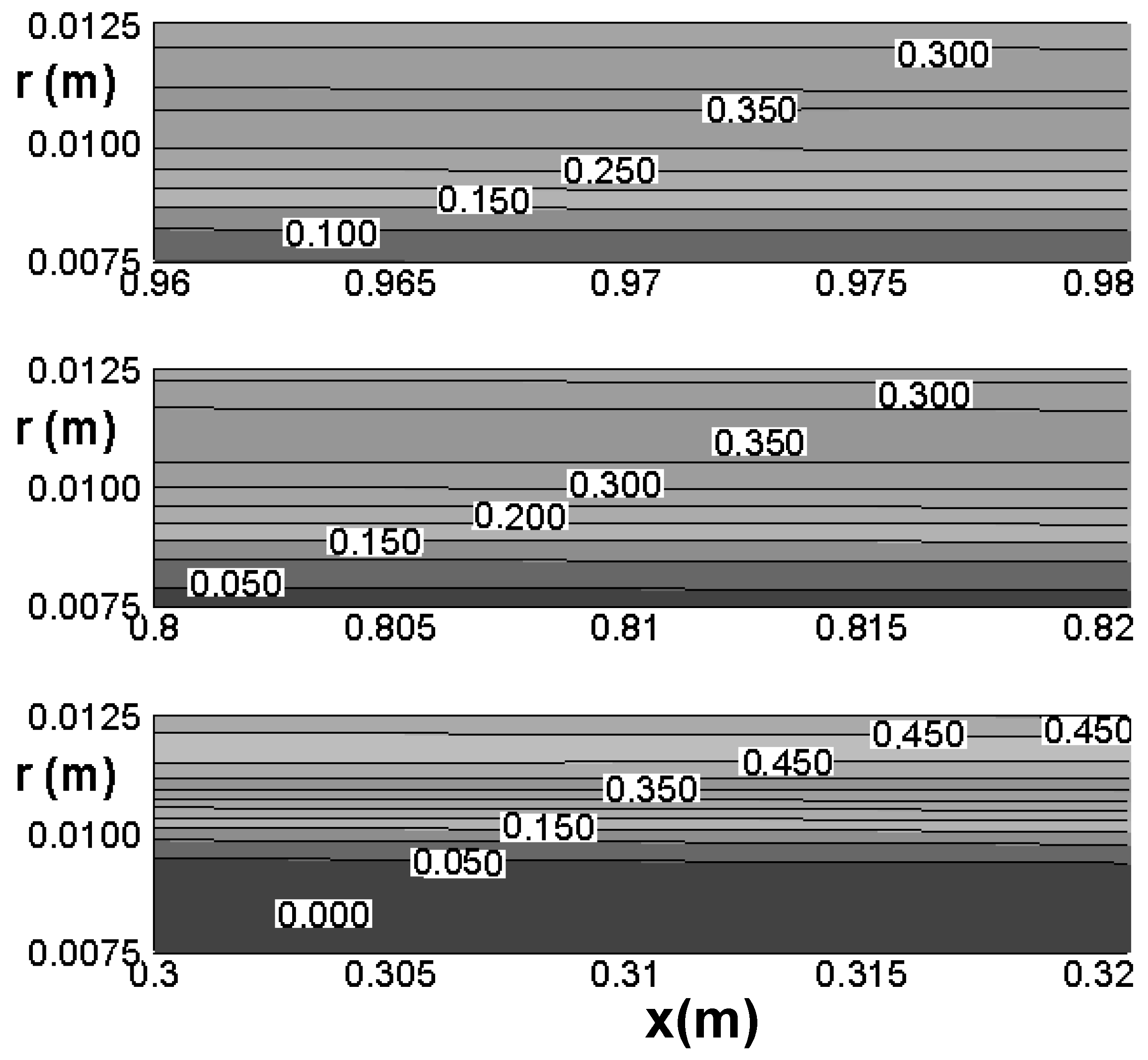
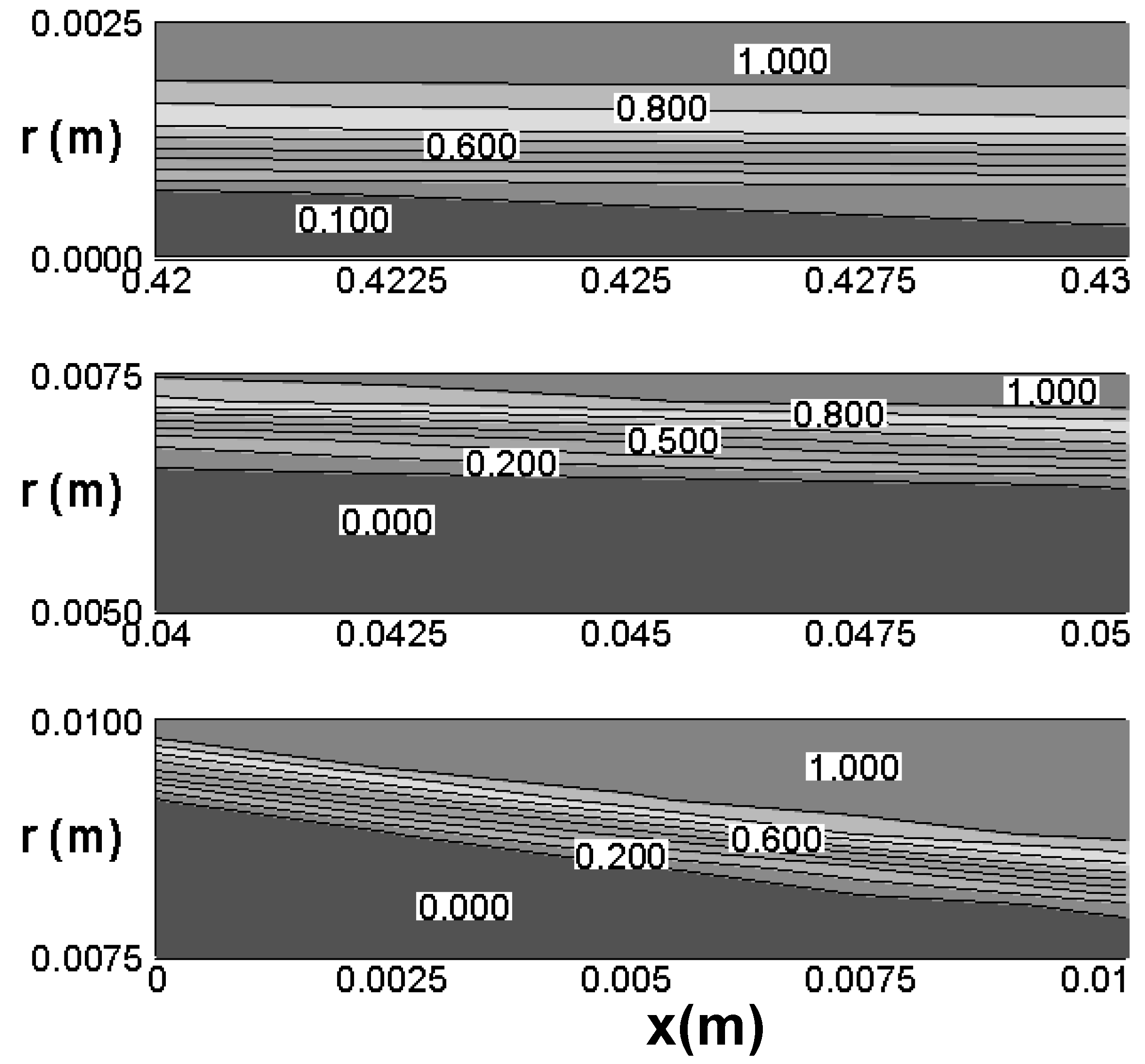
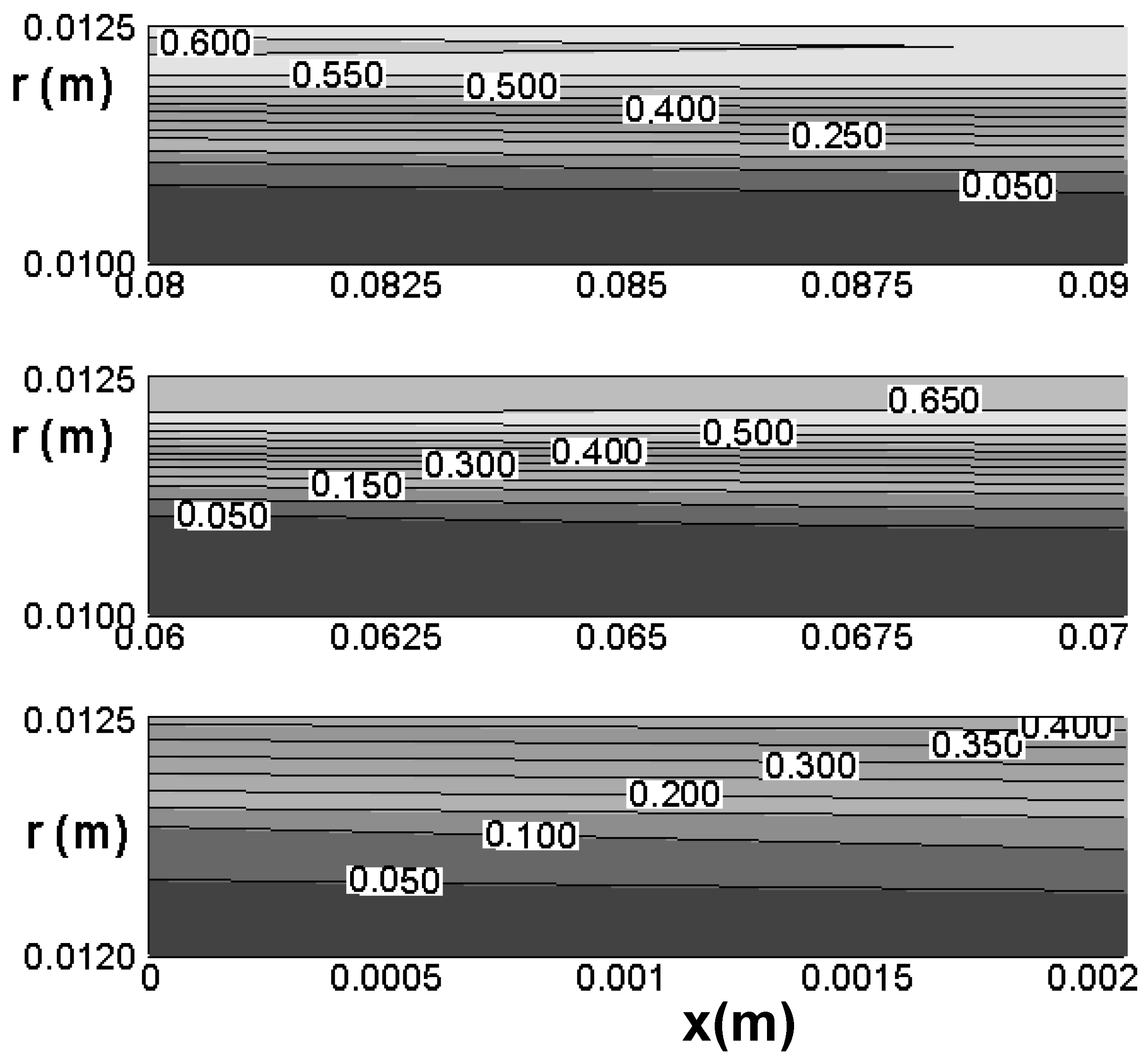
Contour plot for Bejan number at different pipe portions is given in Figure 8. The variation in Bejan number occurs in a narrow band. Near the pipe wall the Bejan number is 1.0 in a fast growing region starting from the entry of the pipe. This indicates that the entropy generation in this region is mainly due to the heat transfer. On the other hand, the Bejan number around the centerline remains zero as expected, since both the temperature and velocity gradients are zero along the centerline. Variation of the entropy generation in different pipe portions is shown in Figure 9 and Figure 10. Entropy generation along the centerline is zero and increases along the radial direction reaching a maximum on the pipe wall. Entropy generation occurs in a region close to the pipe wall which widens along the axial direction.
4. Conclusions
Entropy generation rate in a developing laminar viscous fluid flow in a circular pipe is analyzed. The fluid considered is engine oil and two other fluids namely water and Freon are used in a parametric study. The wall boundary condition is uniform heat flux. The following conclusions can be derived from the current investigation:
- The entropy generation rate is higher near the wall and sharply decreases along the radius away from the surface of the pipe. This is due to the existing temperature and velocity gradients in this region. Around the centerline these gradients are small and therefore the entropy generation is small. Thermal component is the major component in the entropy generation rate.
- The entropy generation along the axial direction near the wall increases sharply to a maximum and then decreases steadily. The integrated value of entropy generation rate over the cross-sectional area of the pipe along the axial direction show a steady increase that is due to the temperature penetration and the widening of the thermal as well as hydrodynamic boundary layers.
- The overall entropy generation rate calculated agrees with the result obtained by control volume thermodynamic analysis within a deviation of 20%. This deviation is attributed to the assumptions made for the thermophysical properties and boundary conditions. This indicated that consideration of variable thermophysical properties may provide more accurate results.
Acknowledgment
The authors acknowledge the support of King Fahd University of Petroleum and Minerals, Dhahran, Saudi Arabia, for this work.
Nomenclature
| Cp | Specific heat (J/kg K) |
| D | Diameter (m) |
| he | Enthalpy at exit (J/kg) |
| hi | >Enthalpy at inlet (J/kg) |
| k | Thermal conductivity (W/m K) |
| L | Length of the duct (m) |
| m | Mass flow rate (kg/s) |
| P | Pressure (N/m2) |
| Pr | Prandtl number ( = µCp/k) |
| q" | Heat flux (W/m2) |
| Q | Total heat transfer rate (W) |
| r | Radial distance (m) |
| Re | Reynolds number ( = pVD / µ ) |
| s | Entropy (J/kg K) |
| se | Entropy at the exit (J/kg K) |
| si | Entropy at the inlet (J/kg K) |
Entropy generation rate (W/K) | |
| T | Temperature (K) |
| Te | Exit fluid temperature (K) |
| Ti | Inlet fluid temperature (K) |
| Tref | Reference temperature (=293 K) |
| Tw | Wall temperature of the duct (K) |
| vr | Radial velocity component (m/s) |
| vz | Axial velocity component (m/s) |
| vz0 | Inlet axial velocity (m/s) |
| V | Fluid bulk velocity (m/s) |
| z | Axial distance (m) |
| Greek Symbols | |
| µ | Viscosity (N s/m2) |
| µref | Viscosity of fluid at reference temperature (N s/m2) |
| ρ | Density (kg/m3) |
| Subscripts | |
| e | exit |
| I | inlet |
| ref | reference value |
| r | radial |
| w | wall |
| z | axial |
References
- Cengel, Y.A.; Boles, M.A. Thermodynamics an Engineering Approach, Second editionMcGraw Hill: New York, 1994. [Google Scholar]
- Bejan, A. A study of entropy generation in fundamental convective heat transfer. ASME Journal of Heat Transfer 1979, 101, 718–725. [Google Scholar] [CrossRef]
- Bejan, A. Entropy Generation Minimization. CRC Press: New York, 1996. [Google Scholar]
- Bejan, A. The concept of irreversibility in heat exchanger design: counterflow heat exchangers for gas-to-gas applications. ASME Journal of Heat Transfer 1977, 99, 374–380. [Google Scholar] [CrossRef]
- Shah, R. K. Compact Heat Exchanger Design Procedures. In Heat Exchangers, Thermal-Hydraulic Fundamentals and Design; Kakac, S., Bergles, A.E., Mayinger, F., Eds.; McGraw Hill: New York, 1981. [Google Scholar]
- Brinkman, H. C. Heat effects in capillary flow. Appl. Sci. Res. Sect. 1951, A2, 120–124. [Google Scholar] [CrossRef]
- Ou, J. W.; Cheng, K. C. Viscous dissipation effects on thermal entrance heat transfer in pipes flows with uniform wall heat flux. Appl. Sci. Res. 1973, 28, 289–301. [Google Scholar]
- Ou, J. W.; Cheng, K. C. Viscous dissipation effects on thermal entrance heat transfer in laminar and turbulent pipe flows with uniform wall temperature. Am. Soc. Mech. Eng. 1974. Pap. 74-HT-50. [Google Scholar]
- Kakac, S.; Bergles, A. E.; Mayinger, F. (Eds.) Heat Exchangers: Thermal-Hydraulic Fundamentals and Design. Hemisphere: Washington, DC, 1981.
- Fraas, A. P. Heat Exchanger Design, 2nd Ed. edWiley: New York, 1989. [Google Scholar]
- Schlunder, E. U. (Ed.) Heat Exchanger Design Handboo. Hemisphere: New York, 1983.
- San, J.-Y.; Jan, C.-L. Second-law analysis of a wet crossflow heat exchanger. Energy 2000, 25(10), 939–955. [Google Scholar] [CrossRef]
- Izquierdo, M.; de Vega, M.; Lecuona, A.; Rodriguez, P. Compressors driven by thermal solar energy: entropy generated, exergy destroyed and exergetic efficiency. Solar Energy 2002, 72(4), 363–375. [Google Scholar] [CrossRef]
- Mahmud, S.; Fraser, R.A. Inherent irreversibility of channel and pipe flows for non-Newtonian fluids. Int. Comm. Heat Mass Transfer 2002, 29, 577–587. [Google Scholar] [CrossRef]
- Nag, P.K.; Kumar, N. Second Law Optimization of Convective Heat Transfer Though a Duct with Constant Heat Flux. Int. J. of Energy Research 1989, 13, 537–543. [Google Scholar] [CrossRef]
- Sahin, A.Z. Second Law Analysis of Laminar Viscous Flow through a Duct Subjected to Constant Wall Temperature. ASME J. Heat Transfer 1998, 120, 76–83. [Google Scholar]
- Sahin, A.Z. The Effect of Variable Viscosity on the Entropy Generation and Pumping Power in a Laminar Fluid Flow through a Duct Subjected to Constant Heat Flux. Heat and Mass Transfer 1999, 35, 499–506. [Google Scholar]
- Bird, R.B.; Stewart, W.E.; Lightfoot, E.N. Transport Phenomena. John Wiley and Sons: New York, 1960. [Google Scholar]
- Mahmud, S.; Fraser, R.A. Irreversibility analysis of concentrically rotating annuli. Int. Comm. Heat Mass Transfer 2002, 29, 697–706. [Google Scholar] [CrossRef]
- Patankar, S. “Numerical Heat Transfer and fluid flow”. Hemisphere, MaGraw-Hill: Washington, 1980. [Google Scholar]
Figure 1.
Schematic view of the pipe.

Figure 2.
Radial velocity profiles at various axial locations.

Figure 3.
Radial temperature profiles at various axial locations.

Figure 4.
Radial entropy generation rate profiles at various axial locations.

Figure 5.
Radial Bejan number profiles at various axial locations.

Figure 6.
Axial temperature profiles at various radial locations.
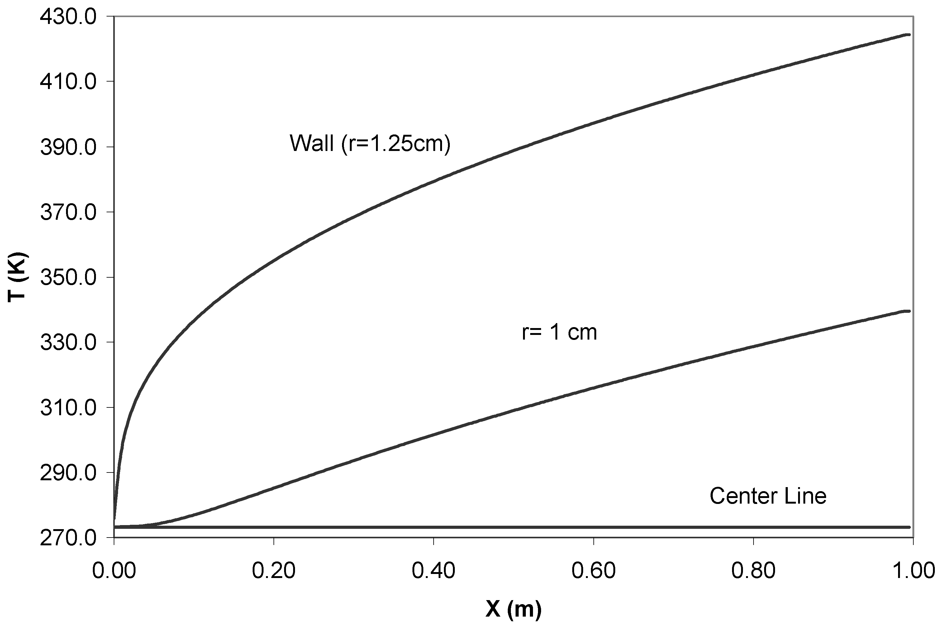
Figure 7.
Axial entropy generation rate profiles at various radial locations.
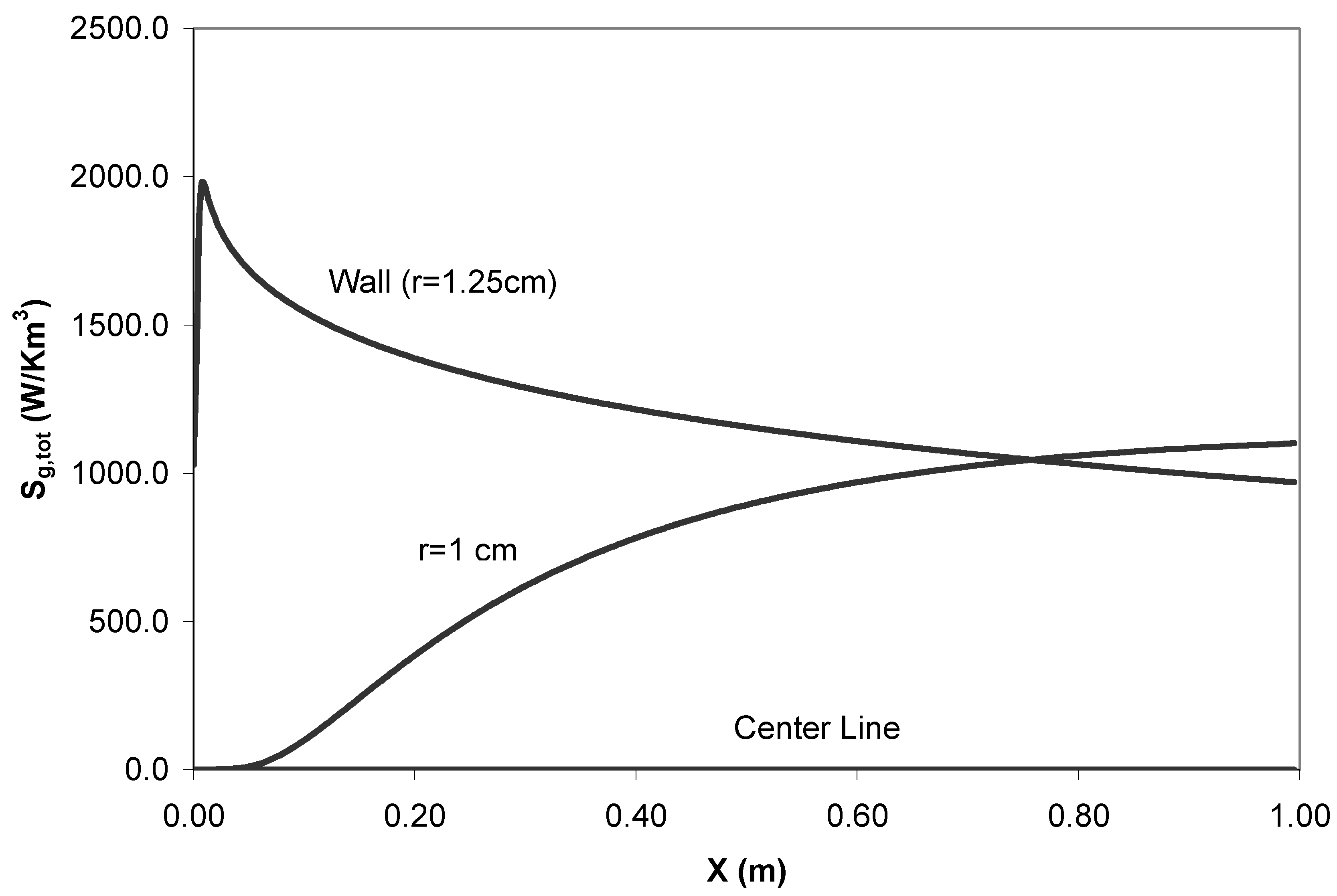
Figure 8.
Bejan Number contours at different pipe portions.

Figure 9.
Modified Entropy Generation () at different pipe inlet portions.

Figure 10.
Modified Entropy Generation () at different pipe inlet portions.

Table 1.
Thermophysical properties of fluids at reference temperature and other parameter used in the analysis.
| Thermophysical parameter | Engine Oil | Water | Freon |
|---|---|---|---|
| Specific heat, Cp (J/ kg K) | 1845 | 4182 | 978.1 |
| Pipe diameter, D (m) | 0.025 | 0.025 | 0.025 |
| Thermal conductivity, k (W/m K) | 0.146 | 0.6 | 0.072 |
| Pipe length, L (m) | 1 | 1 | 1 |
| Wall heat flux, q” (W/m2) | 5000 | 5000 | 5000 |
| Inlet fluid temperature, Ti (K) | 273.15 | 273.16 | 273.16 |
| Reference temperature, Tref (K) | 288.16 | 293 | 300 |
| Inlet axial fluid velocity, vz0 (m/s) | 0.02 | 0.02 | 0.015 |
| Viscosity at reference temperature, µref (N s/m2) | 1.06 | 0.00103 | 0.000254 |
| Density of the fluid, p (kg/m3) | 889 | 998 | 1305.8 |
| Variable | Grid: 30x400 | Grid: 40x500 | % Diff. |
|---|---|---|---|
| Wall temperature at x=0.5m (K) | 388.7770 | 389.0570 | 0.07 |
| Centerline axial velocity at x=0.012 m (m/s) | 0.03861 | 0.03879 | 0.47 |
| Entropy generation on the cross-section at x=0.5m (W/m.K) | 1156.5500 | 1150.6300 | -0.51 |
| Total entropy generation (W/K) | 0.2537 | 0.2542 | 0.18 |
Table 3.
Entropy generation rate integrated over the cross-sectional area of pipe at several axial locations.
| Axial location, x(m) | Entropy Generation rate integrated over cross-sectional area, W/mK | ||
| Engine Oil | Water | Freon | |
| 0 | 0.01328 | 0.00365 | 0.02535 |
| 0.1 | 0.1833 | 0.05532 | 0.23930 |
| 0.5 | 0.2695 | 0.10130 | 0.35620 |
| 0.75 | 0.291 | 0.11527 | 0.37884 |
| 1 | 0.3055 | 0.12520 | 0.39123 |
© 2003 by MDPI (http://www.mdpi.org). Reproduction for noncommercial purposes permitted.
Share and Cite
MDPI and ACS Style
Sahin, A.Z.; Ben-Mansour, R. Entropy Generation in Laminar Fluid Flow through a Circular Pipe. Entropy 2003, 5, 404-416. https://doi.org/10.3390/e5050404
AMA Style
Sahin AZ, Ben-Mansour R. Entropy Generation in Laminar Fluid Flow through a Circular Pipe. Entropy. 2003; 5(5):404-416. https://doi.org/10.3390/e5050404
Chicago/Turabian StyleSahin, Ahmet Z., and Rached Ben-Mansour. 2003. "Entropy Generation in Laminar Fluid Flow through a Circular Pipe" Entropy 5, no. 5: 404-416. https://doi.org/10.3390/e5050404