Entropy and Geometric Objects


ACCESS e.V., Intzestr. 5, D-52072 Aachen, Germany
Entropy 2018, 20(6), 453; https://doi.org/10.3390/e20060453
Submission received: 27 April 2018
/
Revised: 30 May 2018
/
Accepted: 5 June 2018
/
Published: 9 June 2018
(This article belongs to the Special Issue Selected Papers from 4th International Electronic Conference on Entropy and Its Applications)
Abstract
:Different notions of entropy can be identified in different scientific communities: (i) the thermodynamic sense; (ii) the information sense; (iii) the statistical sense; (iv) the disorder sense; and (v) the homogeneity sense. Especially the “disorder sense” and the “homogeneity sense” relate to and require the notion of space and time. One of the few prominent examples relating entropy to both geometry and space is the Bekenstein-Hawking entropy of a Black Hole. Although this was developed for describing a physical object—a black hole—having a mass, a momentum, a temperature, an electrical charge, etc., absolutely no information about this object’s attributes can ultimately be found in the final formulation. In contrast, the Bekenstein-Hawking entropy in its dimensionless form is a positive quantity only comprising geometric attributes such as an area A—the area of the event horizon of the black hole, a length LP—the Planck length, and a factor 1/4. A purely geometric approach to this formulation will be presented here. The approach is based on a continuous 3D extension of the Heaviside function which draws on the phase-field concept of diffuse interfaces. Entropy enters into the local and statistical description of contrast or gradient distributions in the transition region of the extended Heaviside function definition. The structure of the Bekenstein-Hawking formulation is ultimately derived for a geometric sphere based solely on geometric-statistical considerations.
1. Introduction
Different senses of entropy [1] lead to five different notions and perceptions of entropy: the thermodynamic, the information, the statistical, the disorder and the homogeneity senses.
Especially the “disorder sense” and the “homogeneity sense” relate to and require the notion of space and time. There is thus a need to introduce explicit spatial information into formulations of entropy. In general, however, the formulations of entropy used in statistical mechanics or thermodynamics (e.g., Gibbs [2,3], Boltzmann [4]) or in information theory (Shannon [5]) do not comprise of any explicit relation to space or time. A prominent example that actually relates entropy to geometry and space is the Bekenstein-Hawking entropy of a Black Hole. Previous derivations of the Bekenstein-Hawking entropy formula [6] are based, for example, on thermodynamics [7], on quantum theory [8], on statistical mechanics of microstates [9] or on information theory [10,11]. All these derivations (to the best of the author’s knowledge) involve the use of physical entities such as temperature and mass. In contrast, the present article limits itself to the use of only geometric/mathematical information and will derive a formulation revealing a structure that is completely identical to the dimensionless formulation of the Bekenstein-Hawking entropy of a black hole. It is, however, beyond the scope of this article to discuss the host of possible implications of these findings.
The formulation of the entropy of a black hole plays an important role in the holographic principle [12,13] and in current entropic-gravity concepts [14,15] describing gravity as an emergent phenomenon. A review of entropy and gravity, which also comprises a section on the entropy of black holes, is found in [16].
Although developed for describing a physical object—a black hole—having a mass, a momentum, a temperature, a charge, etc., absolutely no information about these attributes of this object can ultimately be found in the final formulation. In contrast, the dimensionless form of the Bekenstein-Hawking entropy SBH is a positive number, which, to obtain the usual form, should be multiplied by Boltzmann’s constant k [17]. The dimensionless formulation, however, only comprises of geometric attributes such as an area A—the area of the black hole’s event horizon, a length LP the Planck length, and a factor of one quarter:
It should thus be possible to construct this formula using a purely geometric approach. Such an approach is attempted in the present article. The approach is based on a continuous 3D extension of the Heaviside function and the phase-field method describing diffuse interfaces.
2. A Geometric Object
A 1D object is a line which is confined by a boundary consisting of two points. A 2D object can be defined as an area being confined by a boundary—the periphery—which is a line. A 3D object is a volume which also is confined by a boundary—its surface—which is an area. Any boundary distinguishes the object region of space from the “non-object” region. For an object with dimension n, its boundary has the dimension n–1. Besides these two fundamental characteristics—bulk and boundary—(e.g., volume/surface, area/periphery, length/endpoints) geometric objects have no further physical attributes. In particular, geometric objects do not have attributes like mass, charge, spin and, further, they do not reveal any intrinsic structure. For reason of simplicity and didactics, the following sections will—without limiting the generality of the concept—limit the discussion to the case of a geometric sphere.
3. Sharp Interface Description of a Geometric Object
A common way of describing a sphere—or any other geometric object—is to use the Heaviside function Θ(x) [18], Figure 1:
The volume V of a sphere with radius r0 in spherical coordinates is then given by
where dΩ is the differential solid angle:
The Heaviside function delimits any contributions of the integrand larger than r0 and thus reduces the boundaries of the integral from infinity to r0:
The surface A of this sphere can be calculated using the gradient of the Heaviside function. Gradients/derivatives of only appear (i.e., have non-zero values) at the positions r0 of the boundaries of an object. In fact, the definition of the Dirac delta function is actually based on the distributional derivative of the Heaviside function Θ(x) [18] as
Using Equation (5) the surface A of the sphere, as well as the surface of more complex geometric objects, can easily be calculated as follows
This is the first term that is relevant for the entropy of the black-hole—the area of the event horizon—i.e., the boundary making the black-hole distinguishable from the “non-black hole”, or a “sphere” distinguishable from the “non-sphere”. The following sections aim to identify a method of deriving, or at least of providing a reason for the other parameters, i.e., for Lp and ultimately for the factor of one quarter, based on a description of a geometric sphere.
4. Phase-Field Description of a Geometric Object
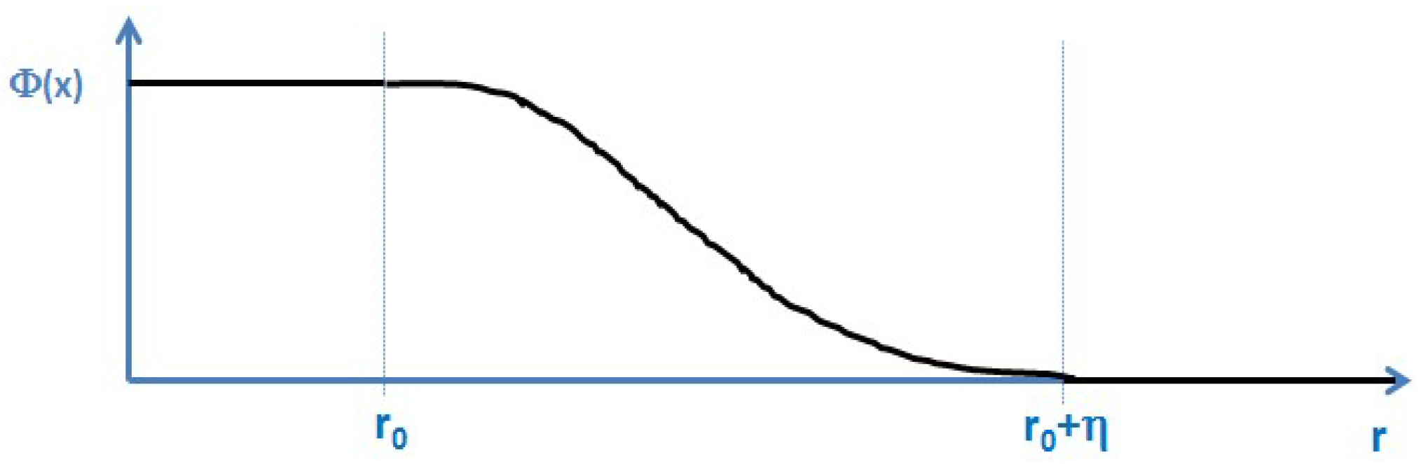
Phase-field models [19,20] developed in recent decades have gained tremendous importance in the area of describing the evolution of complex structures, such as dendrites during phase-transitions. Indeed, they also entered into materials engineering and process design tasks [21]. Similar to the Heaviside function Θ, the phase-field Φ is a field describing the presence or the absence of an object, Figure 2.
In contrast to the Heaviside function that is based on a mathematically discontinuous transition between the two states “1” and “0”, the phase field approach is based on a continuous transition between these two states within a transition zone width η. In case of a very narrow transition width, the phase-field function Φ(x) can be considered as a continuous, differentiable and 3D formulation of the Heaviside function Θ(x):
The gradient symbol without an arrow (∇) here has been used to denote the one dimensional derivative in the radial direction. It is distinguished from a three dimensional gradient that is denoted by the ∇ symbol topped by an arrow (). Thus the left hand side of the equation is a scalar value while the δ-function on the right hand side corresponds to a distribution. A further discussion as to also turning the left-hand side into a distribution is detailed in Section 6.
The shape of the transition in phase-field models depends on the choice of the potential in the model. A double-well potential, for example, leads to a hyperbolic-tangent profile, while a double obstacle potential leads to a cosine profile of the Φ(x) function. However, nothing is known a priori, either about the type of potential or about the shape of this function in the transition region in phase-field models, as seen in Figure 3:
5. Entropy of Interfaces
General considerations about the shape of the phase-field function in the transition region between 0 and η (between r0 and r0 + η, respectively) require continuity of both at the transition to the bulk regions, i.e.:
- is a small, non-zero, positive scaling constant having the unit of a length [L]
- has the dimension of an inverse length [L−1]
- (in one dimension) and (in three dimensions) define the contrast between the two regions. Contrast is a dimensionless, scalar entity and takes values between 0 and 1
- Φ also has no physical units. It takes values between 0 and 1.
The “contrast” will play a particularly important role throughout the following sections. From a philosophical/epistemological point of view, “contrast” provides the basis for any type of categorization or classification and thus the basis for any knowledge. From a physical/mathematical point of view, the contrast’s property of being a dimensionless variable seems to be very important since it can therefore enter into the argument of the logarithm.
5.1. Discrete Descriptions of the Entropy of an Interface
Entropy has revealed its importance in numerous fields. Some of the most important discoveries are based on entropy; such as (i) the Boltzmann factor in energy levels of systems [4]; (ii) the Gibbs energies of thermodynamic phases [2,3]; (iii) the Shannon entropy in information systems [5]; (iv) the Flory-Huggins polymerization entropy in polymers [22]; and (v) the crystallization entropy in metals [23], to name only some of the major highlights. All these approaches using entropy are based on the well-known logarithmic terms (see e.g., [24]):
For a two state system (i = 0, 1), this formula reduces to
On obeying the constraint of probability conservation:
Equation (10) becomes, for a two states system (N = 1)
As a first step towards the description of the entropy of an interface, different models of crystal growth [25]—the Jackson model, the Kossel crystal, and the Temkin model—will be discussed in detail. Here, the interface between a solid and a liquid serves as an instructive example for any type of transition between two different states.
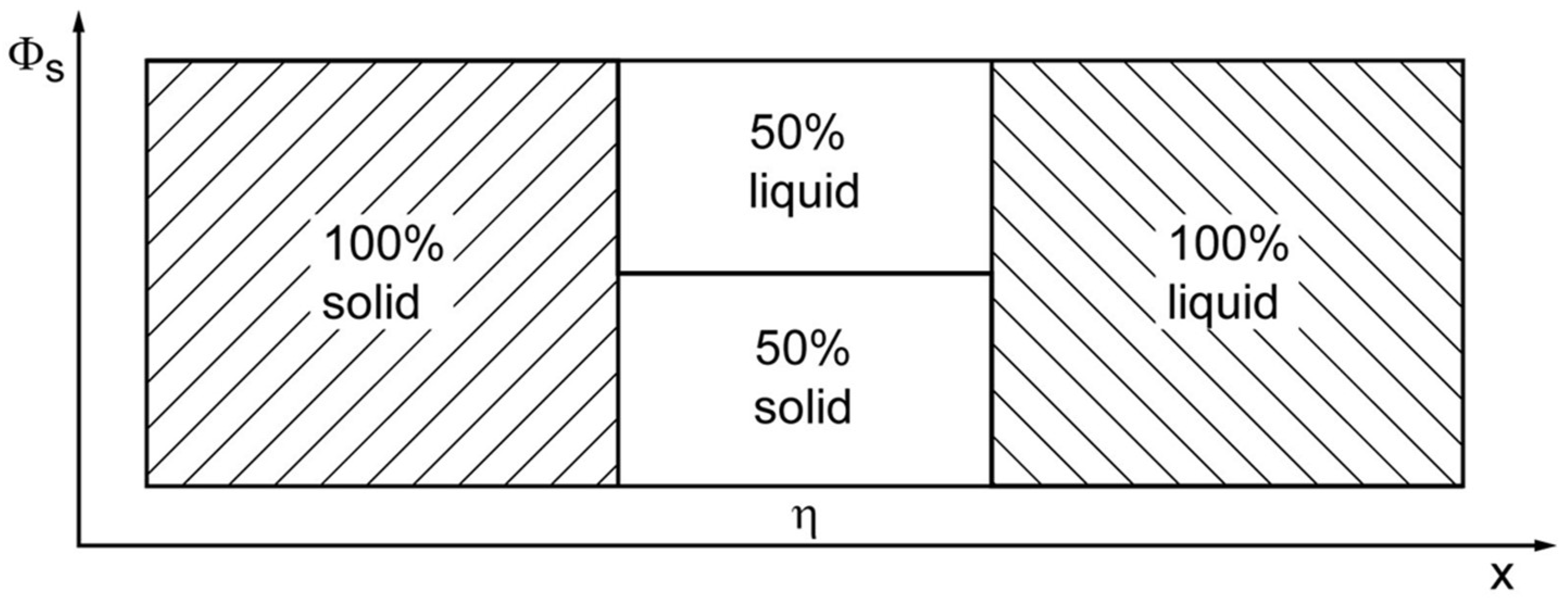
The Jackson model [23] is used to describe the facetted growth of crystals. It assumes an ideal mixing of the two states (solid/liquid) in a single interface layer between the bulk states, Figure 4. The entropy of this interface layer in the Jackson model is described as ideal mixing entropy (see Equations (10) and (12)) which is identical with the Shannon entropy of a binary information system:
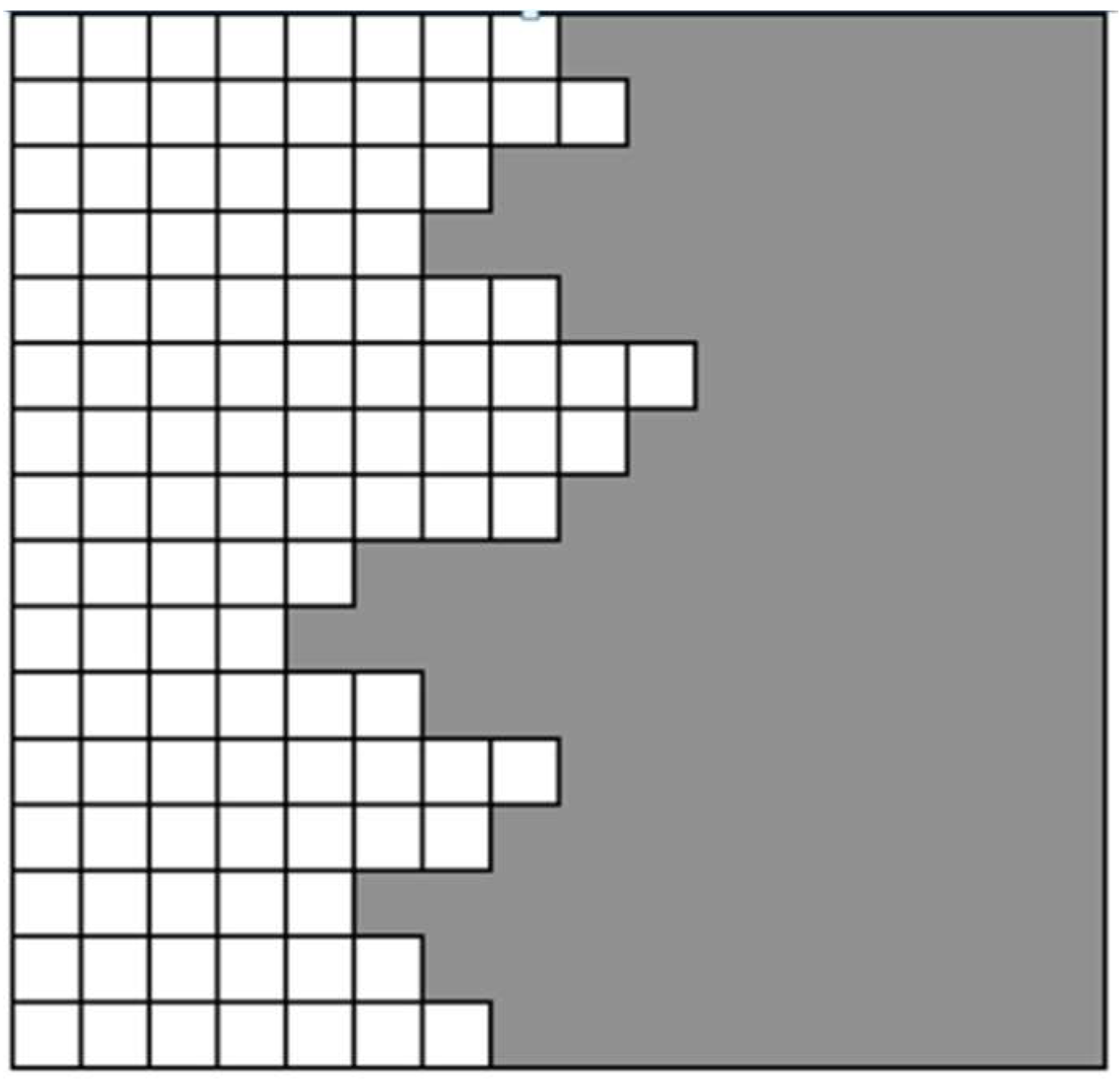
The Kossel model (see, e.g., [25]) is a discrete model that is used to describe the growth of crystals with diffuse interfaces, Figure 5. The Kossel model provides the basis for Temkin’s discrete formulation for the entropy of a diffuse interface.
The Temkin model [27] is used to describe growth of crystals with diffuse interfaces. It assumes ideal mixing between two adjacent states/layers in a multilayer interface. The Temkin model describes the entropy of the diffuse interface as:
This model basically allows for an infinite number of interface layers and recovers the Jackson model as a limiting case for a single interface layer. Accordingly, it represents a more general approach.
Highlighting the importance of the Temkin model, one can state that it introduces neighborhood relations between adjacent layers and thus an “order” or a “disorder” sense. Most important, however, it obviously introduces a gradient and thus a length scale into the formulation of entropy. The gradient in the Temkin model is identified as follows:
where “l” is the distance between two adjacent layers and the gradient is assumed to be constant between these two layers. Actually, Temkin formulated his entropy using the contrast between adjacent layers. An extension of the Temkin model to a continuous formulation and to three dimensions is proposed in the next section.
5.2. From Discrete to Continuous
Temkin’s discrete formula for the entropy of a diffuse interface, as described in the previous section, can be visualized as follows, Figure 6:
The step to a continuous formulation of Temkin’s entropy, that is already described elsewhere [26], corresponds to assuming an averaged and constant value of the gradient between each pair of cells. Variations of the gradient from cell to cell still remain possible. The number of cells may be infinite and the discretization length l may become extremely small. Some useful relations are:
Taking the step from discrete to continuous generates
Substituting
Taking the same steps from one dimension to three dimensions in Cartesian coordinates means (i) extending the radial component product to the full scalar product and (ii) normalizing the other integration directions by some discretization length:
Assuming isotropy of the discretization, i.e.,
ultimately leads to
The factor
can be interpreted as an entropy density.
Expressed in spherical coordinates Equation (22) yields:
Assuming isotropy (i.e., Φ is independent from the angular coordinates), allows one to integrate over the solid angle dΩ
Terms with finite, that is non-zero-values of the ∇Φ yielding contributions to the integral, will only occur at the interface. For very small transition widths η of the phase-field Φ, proportionality between the terms containing ∇Φ and the δ-function can thus be assumed:
This proportionality can be formulated as an equation by introducing a hitherto unknown constant
This equation will be further discussed in the following chapter. By preliminarily inserting this relation into Equation (25) yields
This brings the formulation a step closer to revealing the same structure as the Bekenstein-Hawking entropy. The final step for identifying the factor of one quarter is described in the following section.
6. Gradients in Diffuse Interfaces
Considering in the Temkin model highlighted the importance of gradients or contrast for the formulation of the entropy of a diffuse interface. Hitherto, nothing has been specified about the exact shape of or the radial component of the gradient vector in spherical coordinates ∇rΦ.
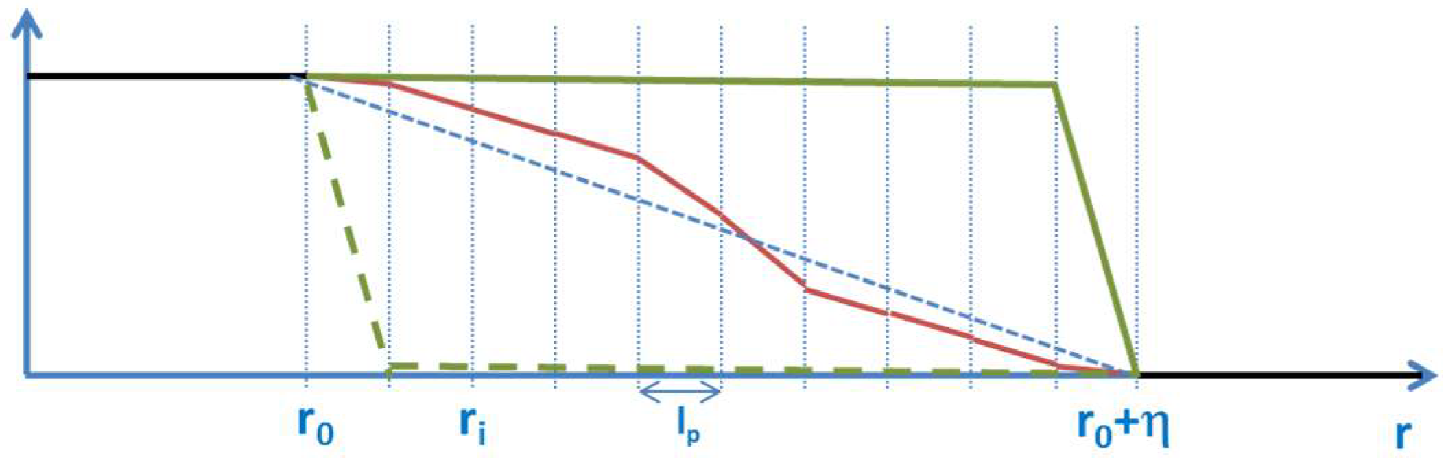
As a first approximation ∇rΦ, could be constant denoting the average gradient between 0 and η (see the blue dashed line in Figure 7). The calculation of this average gradient’s value in a discrete, spatial formulation is
where the number N of the intervals discretizing the interface is defined as
However, this simple approach does not match the continuity requirements for the gradient at the contact points to the bulk regions. It further leads to a statistically improbable, extremely sharp distribution of the contrast; see the blue bar in the histogram in Figure 8.
The average contrast being calculated from an entropy type distribution of contrast reads
The minimum gradient in the distribution has the value 0 (or may be finite but very small; see discussion section) while the maximum gradient is 1/lp. This allows one to fix the boundaries of the integrals to 0 and 1.
This expression, with
yields
The integral of xln(x) gives [28]
When integrating over the interval [0, 1], this integral interestingly yields a value of −¼:
The average gradient or the average contrast resulting from averaging the distribution is thus given by
Replacing the contrast distribution by its average value, i.e., approximating
then yields:
This ultimately leads to
and thus to an expression for the entropy of a geometric sphere SGS revealing the same structure as the Bekenstein-Hawking entropy of a black hole:
7. Summary and Discussion
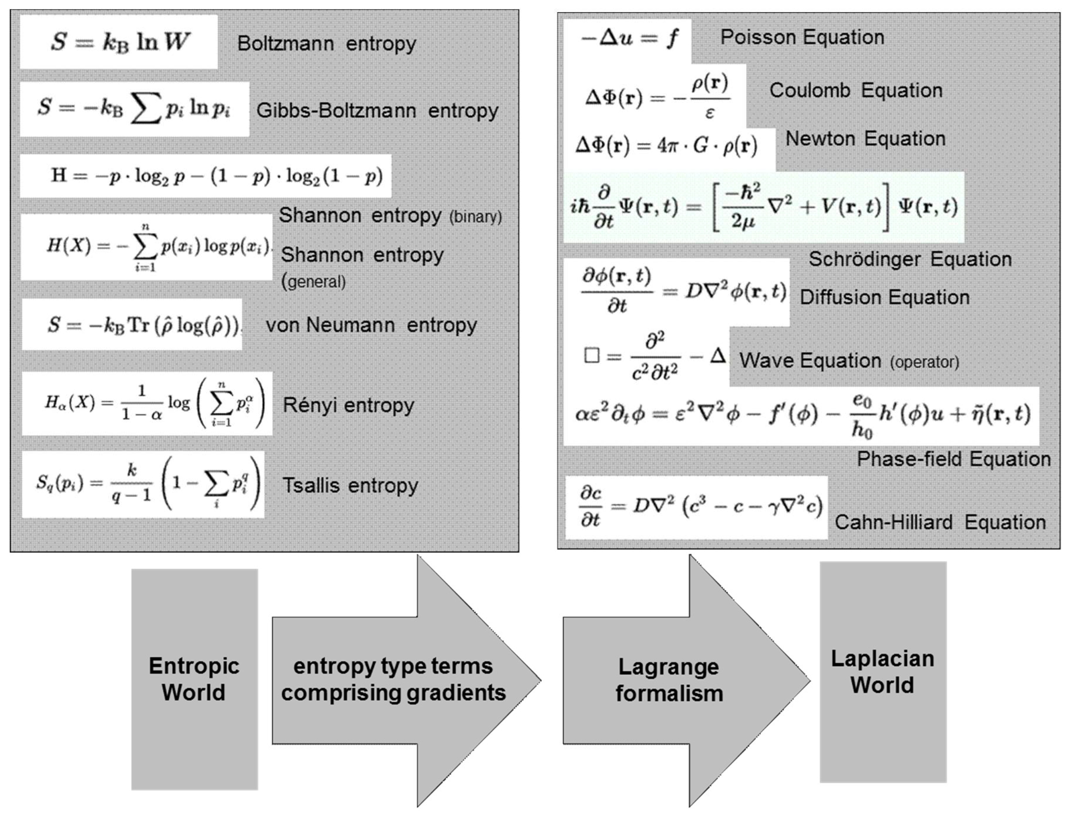
The structure of the Bekenstein-Hawking formula for the dimensionless entropy of a black hole has been derived for the case of a geometric sphere. This derivation is based only on geometric considerations. The key ingredient to the approach is a statistical description of the transition region in a Heaviside or a phase-field function. For this purpose, gradients are introduced in the form of scalar products into the formulation of entropy based on the Temkin entropy of a diffuse interface. This introduces a length scale into entropy and provides a link between the world of entropy type models and the world of Laplacian type models, Figure 9.
The length that is used as the smallest discretization length or as the inverse of the maximum gradient between two states reveals similar characteristics to that of the Planck length.
The minimum gradient—which is set to 0 when making the transition from Equations (28) to (29)—may actually be a finite positive, but non-zero, value. This is calculated as 1/Rmax where Rmax is some characteristic maximum length over which the transition from 1 to 0 occurs. This Rmax might be the radius of the sphere or the radius of the universe outside the sphere. In this case, Equation (33) would contain additional terms leading to minor but perhaps important corrections of the factor of one quarter:
Such corrections become important (i.e., reach values of a few %) if the ratio of lp/Rmax closely approaches 0.1 and might be subject to further discussions. The major implication of the entropy formulation comprising scalar products or gradients, however, are its prospects of providing a link between entropy type models and Laplacian type model equations as outlined in the final section.
The major claims of the presented concept are:
- An entropy can be assigned to any geometric/mathematical object;
- This entropy is proportional to the surface of the object;
- This entropy—in the case of a geometrical sphere—has the same structure as the Bekenstein-Hawking entropy.
The entropy of geometrical objects as described in the present article is based on the discretization of the interface between the object and the non-object into a number of microstates. This implies that this interface is not sharp in a mathematical sense but has to have a finite thickness and thus has to be three dimensional (though being extremely thin in one dimension). A mathematically sharp interface, i.e., a 2D description of interfaces—may be an over—abstraction leading to loss of important information.
It is beyond the scope of the present paper to extend the current description and application range of the Heaviside function or to derive equations of gravity. The paper is meant to show (and does so successfully) that the structure of the Bekenstein-Hawking formula can be derived from mere geometric/statistical considerations. All further interpretations and discussions on how to relate this concept to gravity, to thermodynamics, to quantum physics and many other fields of physics, and probably even mathematics, thus require future discussions in a much broader scientific community.
8. Outlook
Bridging the gap between statistical/entropy type models and spatiotemporal models of the Laplacian world will lead to interesting physics and to new insights (e.g., on entropic gravity), which may emerge when applying and exploiting the proposed “contrast-concept” in more depth.
A first application of this concept [29] already allowed one to derive the Poisson equation of gravitation including terms that are related to the curvature of space. The formalism further generated terms possibly explaining nonlinear extensions known from modified Newtonian dynamics approaches.
Acknowledgments
The ideas documented in the present article have emerged over several years in parallel to ongoing projects being funded by various institutions. A number of stimulating impulses arose from recent discussions about metadata, semantics, ontology, model classifications and other topics in the frame of the European Materials Modelling Council (EMMC-CSA project) being funded by the European Commission under grant agreement n° 723867.
Conflicts of Interest
The author declares no conflict of interest. The founding sponsors had no role in the design of the study; in the collection, analyses, or interpretation of data; in the writing of the manuscript, and in the decision to publish the results.
References
- Haglund, J.; Jeppsson, F.; Strömdahl, H. Different Senses of Entropy—Implications for Education. Entropy 2010, 12, 490–515. [Google Scholar] [CrossRef] [Green Version]
- Willard, G.J. The Scientific Papers of J. Willard Gibbs; Ox Bow Press: Woodbridge, CT, USA, 1993; Volume 1. [Google Scholar]
- Willard, G.J. The Scientific Papers of J. Willard Gibbs; Ox Bow Press: Woodbridge, CT, USA, 1993; Volume 2. [Google Scholar]
- Hasenöhrl, F. Wissenschaftliche Abhandlungen von Ludwig Boltzmann. I. Band (1865–1874) II. Band (1875–1881) and III. Band (1882–1905). Available online: https://phaidra.univie.ac.at/view/o:63647 (accessed on 22 May 2018). (In German).
- Weaver, W.; Shannon, C.E. The Mathematical Theory of Communication; University of Illinois Press: Urbana, IL, USA, 1949; ISBN 0-252-72548-4. [Google Scholar]
- Bekenstein, J.D. Black Holes and Entropy. Phys. Rev. D 1973, 7, 2333. [Google Scholar] [CrossRef]
- Bekenstein, J.D. Black-hole thermodynamics. Phys. Today 1980, 33, 24–31. [Google Scholar] [CrossRef]
- Hawking, S.W. The quantum mechanics of black holes. Sci. Am. 1977, 236, 34–42. [Google Scholar] [CrossRef]
- Strominger, A.; Vafa, C. Microscopic origin of the Bekenstein-Hawking entropy. Phys. Lett. B 1996, 37, 99–104. [Google Scholar] [CrossRef]
- Bekenstein, J.D. Black holes and information theory. Contemp. Phys. 2004, 45, 31–43. [Google Scholar] [CrossRef] [Green Version]
- Bekenstein, J.D. Information in the holographic universe. Sci. Am. 2003, 289, 58–65. [Google Scholar] [CrossRef] [PubMed]
- Hooft, G.’T. Dimensional Reduction in Quantum Gravity. arXiv, 1993; arXiv:gr-qc/9310026. [Google Scholar]
- Bousso, R. The holographic principle. Rev. Mod. Phys. 2002, 74, 825–874. [Google Scholar] [CrossRef]
- Verlinde, E.P. On the Origin of Gravity and the Laws of Newton. J. High Energy Phys. 2011, 29, 1–17. [Google Scholar] [CrossRef]
- Verlinde, E.P. Emergent Gravity and the Dark Universe. arXiv, 2016; arXiv:1611.02269. [Google Scholar]
- Grøn, Ø. Entropy and Gravity. Entropy 2012, 14, 2456–2477. [Google Scholar] [CrossRef] [Green Version]
- Bekenstein, J.D. Bekenstein-Hawking entropy. Scholarpedia 2008, 3, 7375. [Google Scholar] [CrossRef]
- Heaviside Step Function. Available online: https://en.wikipedia.org/wiki/Heaviside_step_function (accessed on 10 November 2017).
- Provatas, N.; Elder, K. Phase-Field Methods in Materials Science and Engineering; Wiley VCH: Weinheim, Germany, 2010. [Google Scholar]
- Steinbach, I. Phase-field models in Materials Science-Topical Review. Model. Simul. Mater. Sci. Eng. 2009, 17, 073001. [Google Scholar] [CrossRef]
- Schmitz, G.J.; Böttger, B.; Eiken, J.; Apel, M.; Viardin, A.; Carré, A.; Laschet, G. Phase-field based simulation of microstructure evolution in technical alloy grades. Int. J. Adv. Eng. Sci. Appl. Math. 2010, 2, 126–129. [Google Scholar] [CrossRef]
- Flory, P.J. Principles of Polymer Chemistry; Cornell University Press: New York, NY, USA, 1953. [Google Scholar]
- Jackson, K.A. Liquid Metals and Solidification; ASM: Cleveland, OH, USA, 1958. [Google Scholar]
- Jaynes, E.T. Probability Theory: The Logic of Science. Available; Cambridge University Press: Cambridge, UK, 2003; Chapter 11. [Google Scholar]
- Woodruff, D. The Solid Liquid Interface; Cambridge University Press: Cambridge, UK, 1973. [Google Scholar]
- Schmitz, G.J. Thermodynamics of Diffuse Interfaces. In Interface and Transport Dynamics; Emmerich, H., Nestler, B., Schreckenberg, M., Eds.; Springer Lecture Notes in Computational Science and Engineering; Springer: Berlin/Heidelberg, Germany, 2003; pp. 47–64. [Google Scholar]
- Temkin, D.E. Crystallization Processes; Sirota, N.N., Gorskii, F.K., Varikash, V.M., Eds.; Consultants Bureau: New York, NY, USA, 1966. [Google Scholar]
- Bronstein, I.N.; Mühlig, H.; Musiol, G.; Semendjajew, K.A. Taschenbuch der Mathematik (Bronstein); Deutsch, H., Ed.; Verlag: Harri Deutsch, Germany, 2016. [Google Scholar]
- Schmitz, G.J. A combined entropy/phase-field approach to gravity. Entropy 2017, 19, 151. [Google Scholar] [CrossRef]
Figure 1.
Schematic of the Heaviside function Θ(x). This function takes the value 1 wherever the object/sphere is present and is 0 elsewhere.
Figure 1.
Schematic of the Heaviside function Θ(x). This function takes the value 1 wherever the object/sphere is present and is 0 elsewhere.
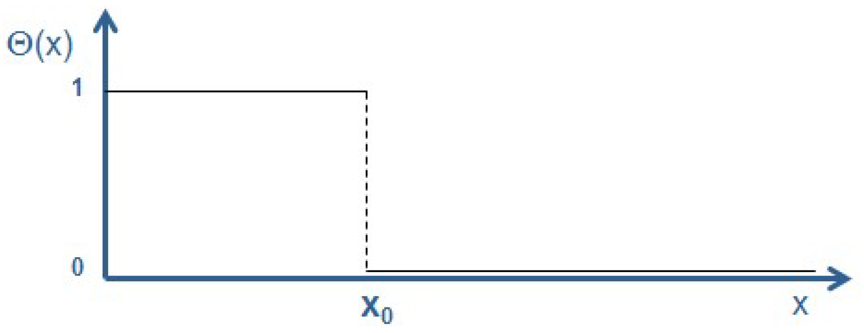
Figure 2.
Schematic of the phase-field function Φ(x). This function takes the value 1 wherever the object/sphere is present and is 0 elsewhere. In contrast to the Heaviside function it reveals a continuous transition over a finite—though very small—interface thickness η.
Figure 2.
Schematic of the phase-field function Φ(x). This function takes the value 1 wherever the object/sphere is present and is 0 elsewhere. In contrast to the Heaviside function it reveals a continuous transition over a finite—though very small—interface thickness η.

Figure 3.
Nothing is known a-priori about the shape of the functions in the small transition zone between the two states. It should also be noted that two state systems have a major importance in quantum mechanical systems and transitions.
Figure 3.
Nothing is known a-priori about the shape of the functions in the small transition zone between the two states. It should also be noted that two state systems have a major importance in quantum mechanical systems and transitions.
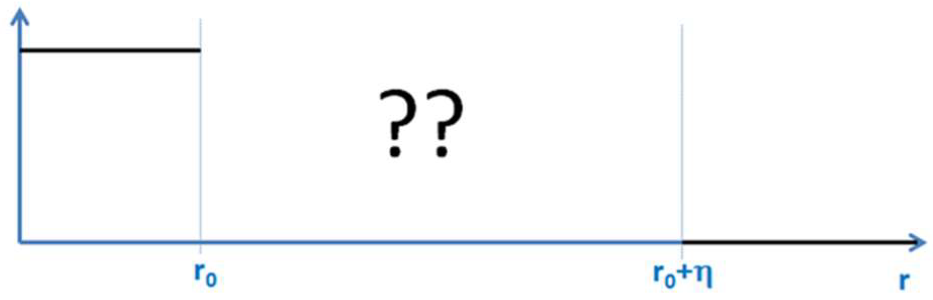
Figure 4.
The entropy distribution of the Jackson model generates Φ = 0.5 as the most probable value in the interface region (adapted from [26]).
Figure 4.
The entropy distribution of the Jackson model generates Φ = 0.5 as the most probable value in the interface region (adapted from [26]).

Figure 5.
The Kossel model assumes attachment of solid only on the existing solid, i.e., it does not allow for any overhang. Using multiple layers, this model describes a stepwise transition from 100% solid (the four left layers) to 100% liquid (from layer 11 to the right). The projection of layers five to 10 yields a decreasing fraction of solid with increasing layer numbers (adapted from [26]).

Figure 6.
The values of the Temkin model visualized as contrast, i.e., (in green).
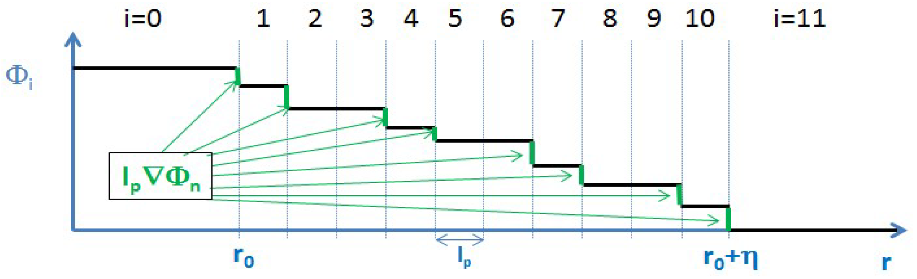
Figure 7.
Possible profiles of the Φ function in the transition region. These different shapes lead to different distributions of contrast (see Figure 8).
Figure 7.
Possible profiles of the Φ function in the transition region. These different shapes lead to different distributions of contrast (see Figure 8).

Figure 8.
Distributions of contrast in the transition region for the different profiles depicted in Figure 7 : A constant average gradient (blue) leads to an extremely narrow distribution of contrast centered at lp/η. The green shapes lead to high counts for small contrast. The red shape leads to a broad distribution of small and high contrast values. An entropy type distribution of contrast xi (N = 10): H(x) = −10xln(x), is indicated as the red-line overlay.
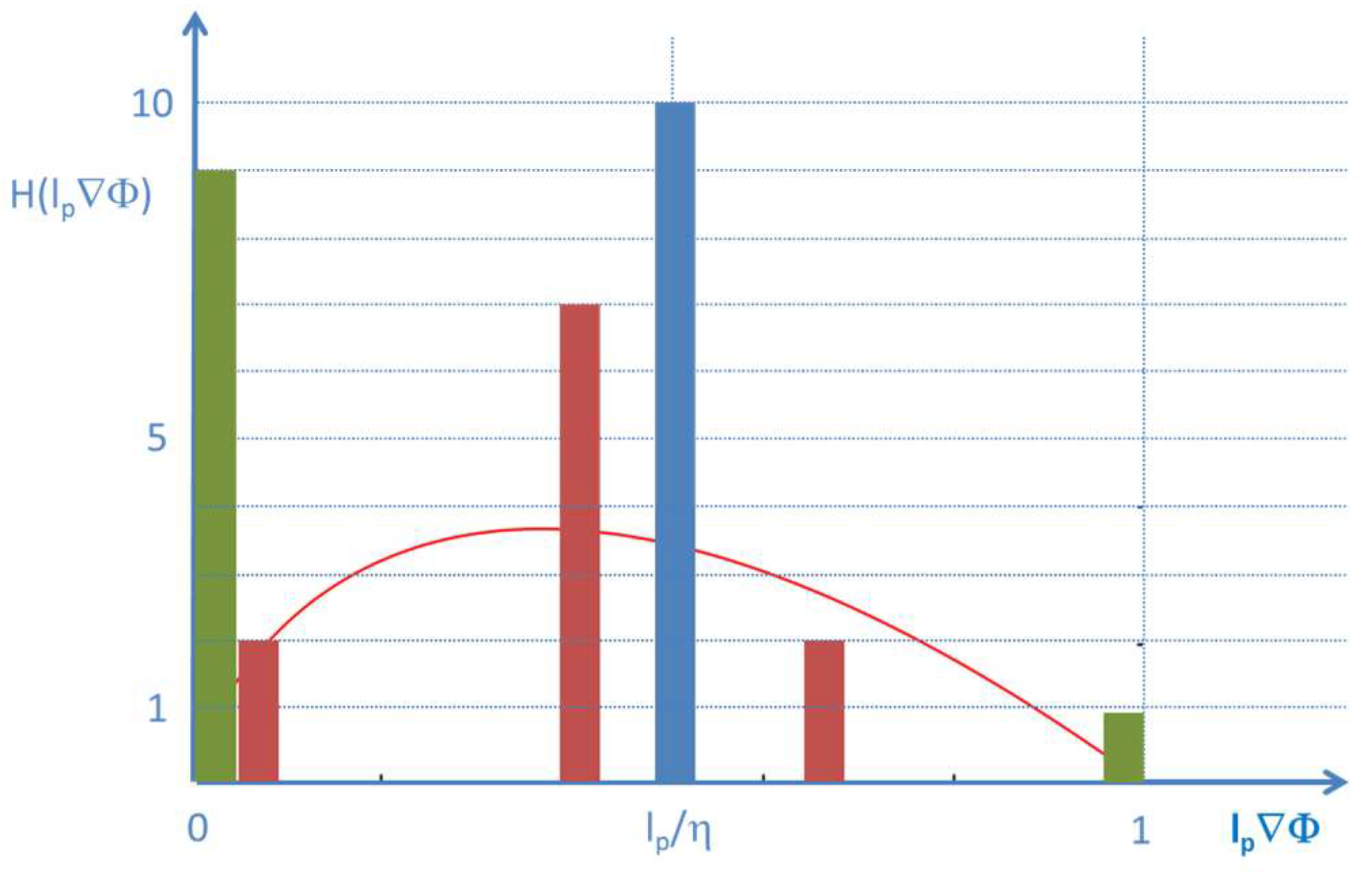
Figure 9.
(Upper left) Incomplete list of models for a statistical/entropic description of entities in physics and in information theory. Most of these models reveal a logarithmic term as a common ingredient. None of these expressions comprises of gradients and/or Laplacian operators; (Upper right) Incomplete list of models for a spatiotemporal description of stationary solutions or for the evolution in physical systems. Many of these models have a Laplacian operator as a common ingredient; (Bottom) Entropy formulations comprising gradients, as depicted in the present paper, provide a bridge between these two model worlds.

© 2018 by the author. Licensee MDPI, Basel, Switzerland. This article is an open access article distributed under the terms and conditions of the Creative Commons Attribution (CC BY) license (http://creativecommons.org/licenses/by/4.0/).
Share and Cite
MDPI and ACS Style
Schmitz, G.J. Entropy and Geometric Objects. Entropy 2018, 20, 453. https://doi.org/10.3390/e20060453
AMA Style
Schmitz GJ. Entropy and Geometric Objects. Entropy. 2018; 20(6):453. https://doi.org/10.3390/e20060453
Chicago/Turabian StyleSchmitz, Georg J. 2018. "Entropy and Geometric Objects" Entropy 20, no. 6: 453. https://doi.org/10.3390/e20060453
Note that from the first issue of 2016, this journal uses article numbers instead of page numbers. See further details here.