Applying Discrete Homotopy Analysis Method for Solving Fractional Partial Differential Equations


Bolvadin Vocational School, Afyon Kocatepe University, 03300 Afyonkarahisar, Turkey
Entropy 2018, 20(5), 332; https://doi.org/10.3390/e20050332
Submission received: 3 March 2018
/
Revised: 27 April 2018
/
Accepted: 27 April 2018
/
Published: 1 May 2018
(This article belongs to the Special Issue Wavelets, Fractals and Information Theory III)
Abstract
:In this paper we developed a space discrete version of the homotopy analysis method (DHAM) to find the solutions of linear and nonlinear fractional partial differential equations with time derivative . The DHAM contains the auxiliary parameter , which provides a simple way to guarantee the convergence region of solution series. The efficiency and accuracy of the proposed method is demonstrated by test problems with initial conditions. The results obtained are compared with the exact solutions when . It is shown they are in good agreement with each other.
1. Introduction
Fractional calculus has been of increasing interest to scientists and engineers, arising in mathematical physics, chemistry, modeling mechanical and electrical properties of real phenomena [1,2,3,4,5,6]. Fractional calculus has been recognized as a powerful instrument to discover the secret directions of various material and physical processes that deal with derivatives and integrals of arbitrary orders [7,8,9,10,11,12,13,14,15,16].
Various techniques have been investigated to solve partial differential equations of fractional order, such as the homotopy analysis method (HAM) [17,18,19,20,21,22], homotopy perturbation method (HPM) [23,24,25,26], Adomian decomposition method (ADM) [27,28,29], meshless method [30,31,32,33], operational matrix [34,35] and so on. In 1992, Liao introduced the homotopy analysis method, a semi-analytical method, for solving strongly nonlinear differential equations [20]. The main advantage of HAM is that it provides great freedom to choose equation type and solution expression of related linear high-order approximation equations. HAM gives rapidly convergent successive approximations of the exact solutions, if such a solution exists, otherwise approximations can be used for numerical purposes. It is an analytical approach to get the series solution of linear and nonlinear partial differential equations. Unlike the other analytical techniques, HAM is independent of small/large physical parameters. Since HAM has many advantages in comparison to other analytical methods, it is employed to solve continuous problems. Hence after the discrete ADM method [36], the discrete homotopy analysis method (DHAM) was introduced in 2010 by Zhu et al. [37]. This method can be applied to complex problems containing discontinuity in fluid characteristics and geometry of the problem. In addition, it needs little computational cost as numerical method in comparison to HAM; as an analytical approach DHAM has similar advantages to continuous HAM. By means of introducing an auxiliary parameter one can adjust and control the convergence region of the solution series. This method should be employed for solving various differential equations to highlight its high capabilities in comparison with other numerical methods.
In this study, we develop the discrete homotopy analysis method (DHAM) for the fractional discrete diffusion equation, nonlinear fractional discrete Schrödinger equation and nonlinear fractional discrete Burgers’ equation with time derivative . The approximate analytical solutions of the test problems are obtained using initial conditions. The obtained solutions are verified by comparison with exact solution when .
2. Preliminaries and Notations
2.1. Fractional Analysis
Definition 1
([38]). A real function is said to be in space if there exists a real number such that where .
Definition 2
([38]). A function is said to be in space if .
Definition 3
([5]). Let and then Riemann-Liouville fractional integral of with respect to t of order is denoted by and is defined as
The well-known property of Riemann-Liouville operatoris
Definition 4
([39]). Form to be the smallest integer that exceeds the Caputo fractional derivative of with respect to t of order is defined as
Note that the Caputo fractional derivative is considered due to its suitable for initial conditions of the differential equations.
The relations between Riemann-Liouville operator and Caputo fractional differential operator are given as follows
2.2. Discrete Homotopy Analysis Method
Consider the following general difference equation respect to j
where is a linear or nonlinear operator, j and t denote the independent variables. Suppose that and the function is the discrete function and denoted by .
For simplicity, we ignore all boundary or initial conditions, which can be treated in the similar way. Similarly to continuous HAM, we first construct the so-called zeroth-order deformation equation by means of the discrete HAM (DHAM)
where is an embedding parameter, is an auxiliary parameter, is an auxiliary linear operator, is an initial guess of denotes a nonzero auxiliary function, is an unknown function about j, t, p. It is important that one has great freedom to choose auxiliary things in (2). Obviously, when and it holds
respectively. Thus, as p increases from 0 to 1, the solution varies from initial guess to the solution . Expanding in Taylor series with respect to p, we have
where
Similarly continuous HAM by Liao [21], if the auxiliary linear operator, the initial guess, the auxiliary parameter and the auxiliary function are so properly chosen, the series (3) converges at then we have
As and Equation (2) becomes
which is used in the discrete homotopy perturbation method (DHPM) [16], where as the solution obtained directly, without using Taylor series.
According to Equation (4), the governing equation can be deduced from the zeroth-order deformation Equation (DHAM). Define the vector
Differentiating the zeroth-order deformation Equation (2) m times with respect to the embedding parameter p and then setting p = 0 and finally dividing them by m!, we obtain the following mth-order deformation equation:
where
and
It should be emphasized that it is very important to ensure that Equation (3) converges at otherwise, the Equation (5) has no meaning.
Theorem 1 (Convergence Theorem).
As long as the series (5) is convergent, where is governed by the high deformation Equation (6). It must be the solution of the original Equation (1).
Proof.
If the series is convergent, we can write
and it holds
From the mth-order deformation Equation (6) and by using the definition of it yields
Since then
On the other side, according to the definition (7), we have
In general, doesn’t satisfy the original Equation (1). Let
denote the residual error of Equation (1). Obviously,
corresponds to the exact solution of the Equation (1).
According to the above definition, the Maclaurin series of the residual error with respect to the embedding parameter p is
when , the above expression gives
That is, according to the definition of we have the exact solution of the original Equation (1) when . Thus as long as the series
is convergent, it must be the solution of the original Equation (1). ☐
3. Examples
Example 1.
Consider the time fractional discrete diffusion equation
with initial condition
Discrete diffusion equation is widely used in applied sciences. For example, population growth modeled by geographical spread [40], to model ionic diffusion on a lattice [41], and so on. Moreover, the entropy production was calculated for fractional diffusion Equation [42,43].
The standard central differences and are defined by
Initial value problem (13) and (14) is the discrete form of initial value problem for diffusion equation
with initial condition
whereis Caputo fractional derivative of order.
To solve Equation (13) by DHAM let us consider the following linear operator:
with the property that
where c is constant coefficients. We define the nonlinear operator as
Using the above definition, we construct the zeroth-order deformation equation by Equation (2).
It is obvious that when the embedding parameterand, Equation (2) becomes
respectively. Then we obtain the mth-order deformation equation for with
where
For simplicity, we selectin this problem. So, the approximations ofare only depend on auxiliary parameter.
Solve the above equation under the initial condition
we get
Thus the rest of componentsof the DHAM can be completely obtained. So, we approximate the analytical solution
Setting, we get an accurate approximation solution in the following form:
whereis Mittag-Leffler function.
is the exact solution of the continuous form.
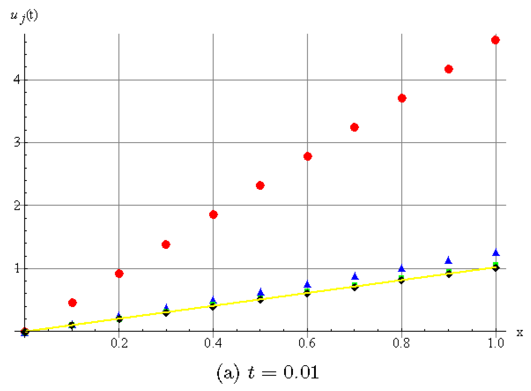
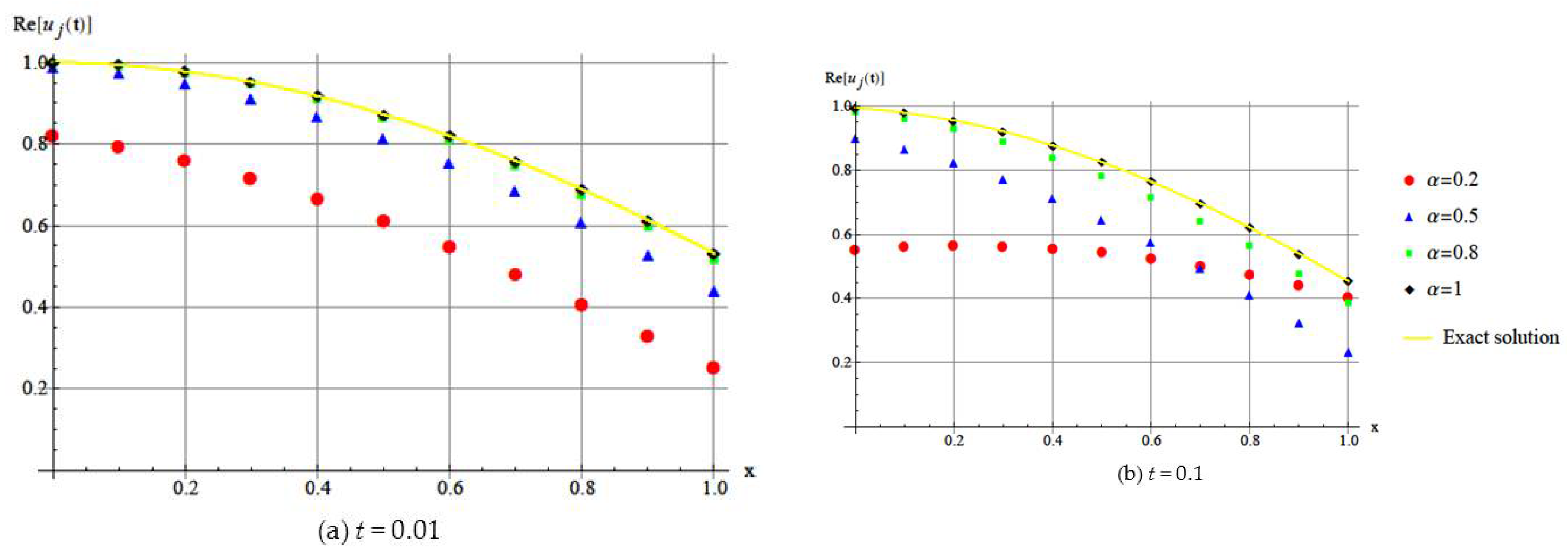
Figure 1 shows the DHAM approximate solution of for different values of .
We can see that different fractional order lead to different diffusion behaviors.
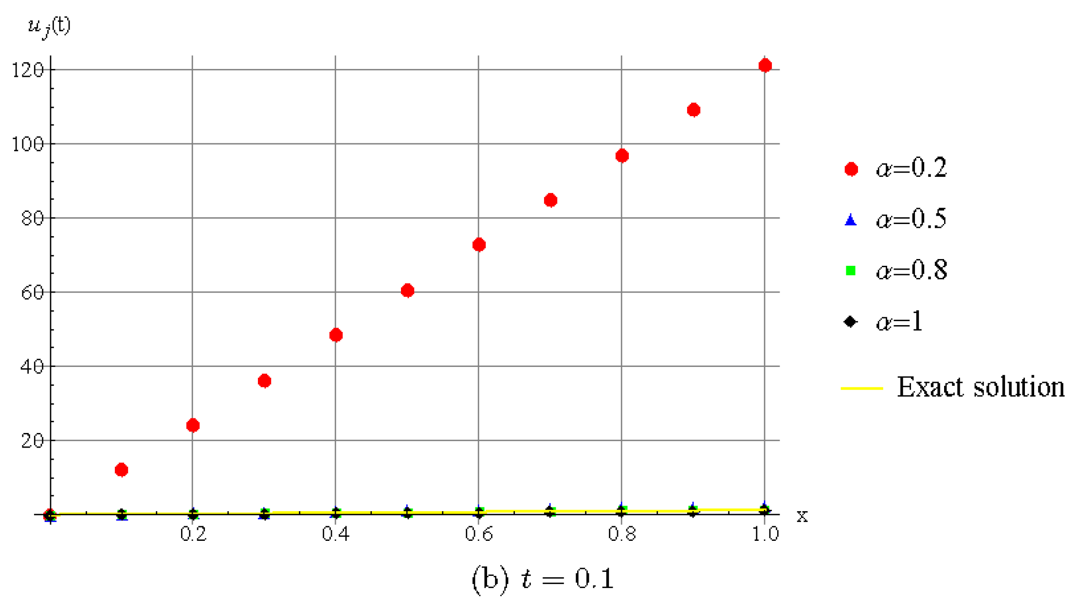
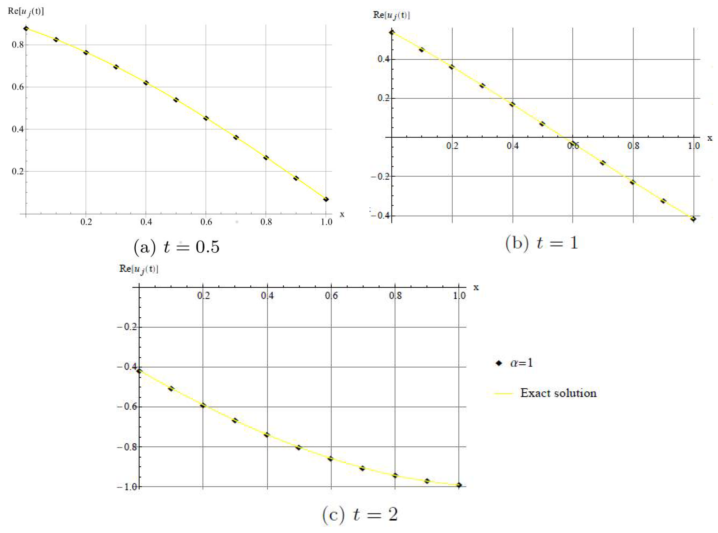
In Figure 2, we show that the method has good agreement with the exact solution when .
Example 2.
Consider the nonlinear fractional discrete Schrödinger equation
with initial condition
Discrete nonlinear Schrödinger equation is widely used in applied sciences. Describing the propagation of electromagnetic waves in glass fibers, one–dimensional arrays of coupled optical waveguides [18] and light–induced photonic crystal lattices [44]. Moreover, they are an established model for optical pulse propagation in various doped fibers [45,46].
Discrete nonlinear Schrödinger equations are also called lattice nonlinear Schrödinger equations [47].
The parameteris called (discrete) dispersion and the parameter q is called anharmonicity.
Initial value problem (19) and (20) is the discrete form of initial value problem for Schrödinger equation
with initial condition
we set .
By means of DHAM, we choose the linear operator:
with propertywhere c is constant. We define the nonlinear operator as
we construct the zeroth-order deformation equation by Equation (2).
Forand, we can write
respectively. Thus, we obtain the mth-order deformation equation
where
we can select again. Thus, the approximations ofare only depend on auxiliary parameter.
Therefore the solution of the mth-order deformation Equation (23) forbecome
Substituting the initial condition (20) into the system (25), we get
where(discrete dispersion relation).
Thus, we can conclude that
Setting, we get an accurate approximation solution in the following form:
For the special casethe form Equation (26) is obtained discrete plane wave solution
which is the same solution obtained in [6].
is the plane wave solution of the continuous form, where k is the wave number anddenotes the frequency.
We can observe the different behaviors of the discrete fractional Schrödinger equations, with different fractional parameters.
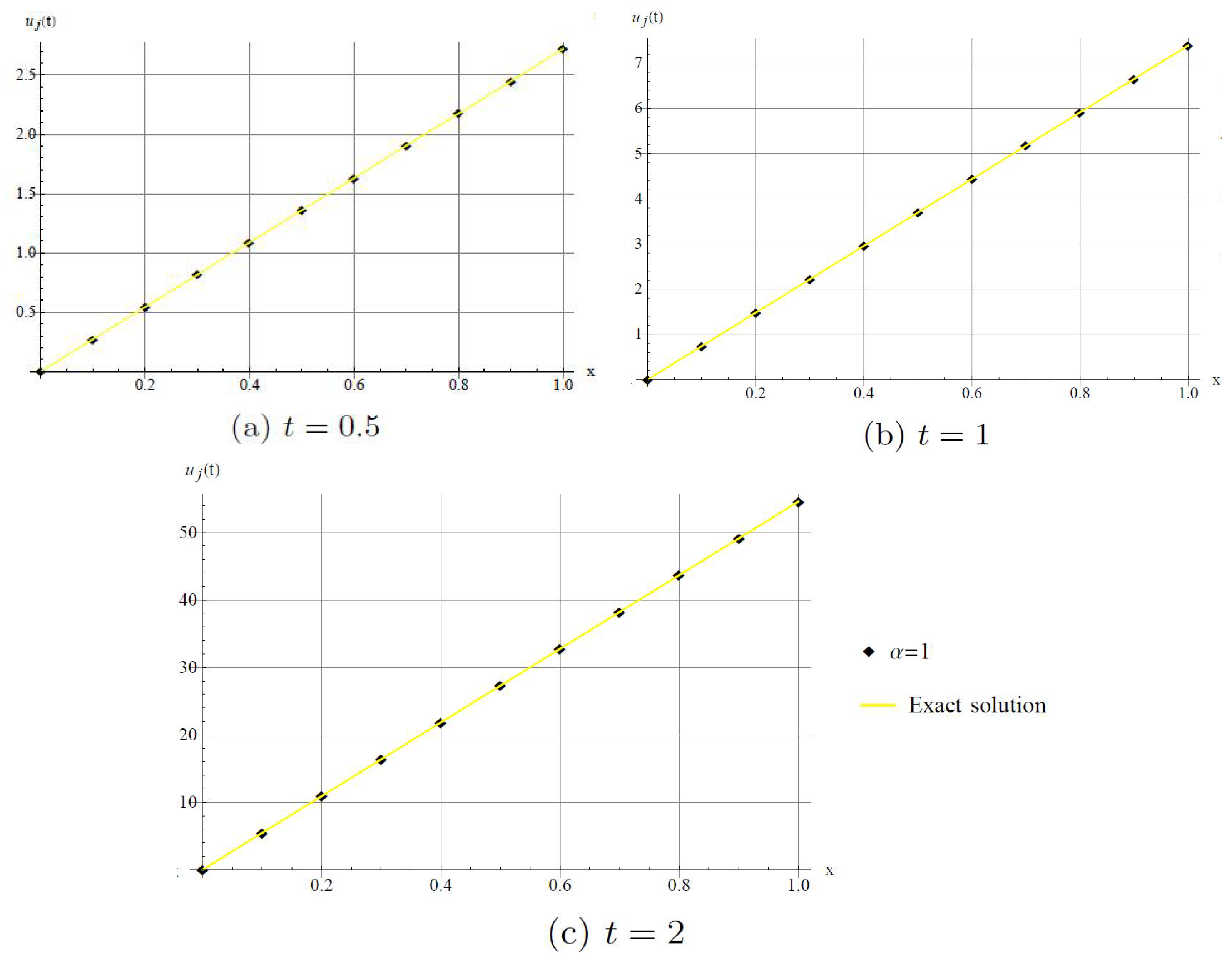
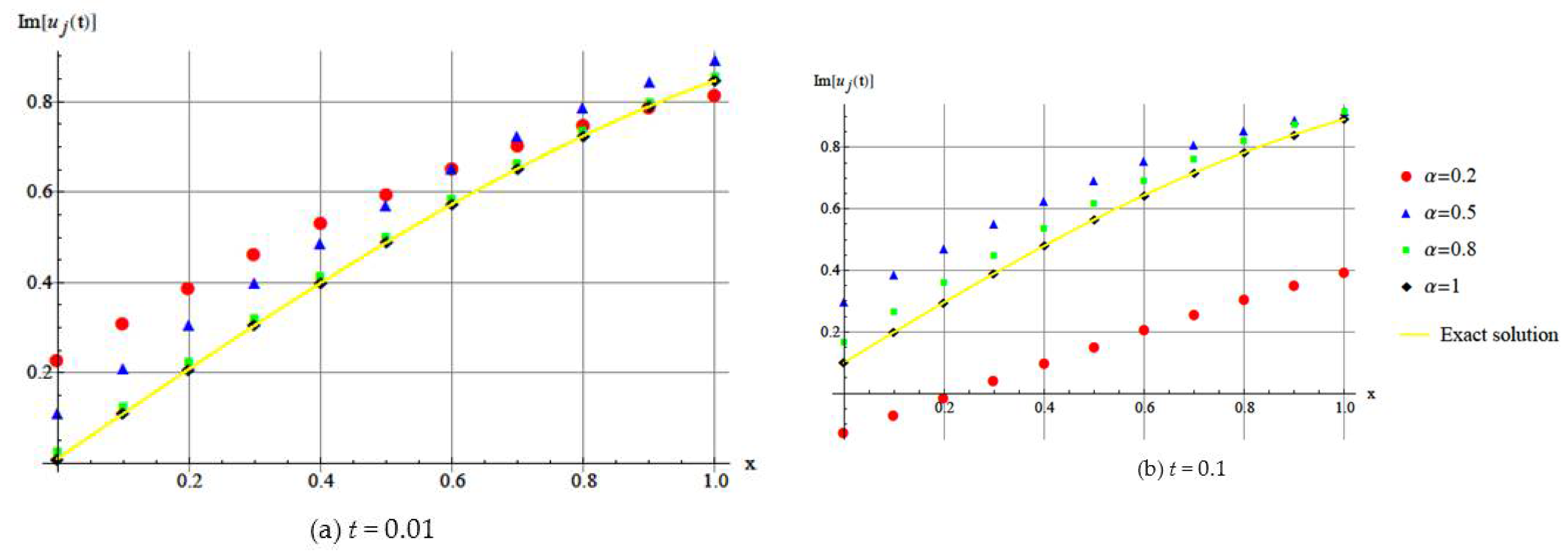
In Figure 5, we show that the method has good agreement with imaginary part of the exact solution when .
In Figure 6, we show that the method has good agreement with real part of the exact solution when .
Example 3.
Consider time fractional space discrete nonlinear Burgers’ equation
with initial condition
Initial value problem (27) and (28) is the discrete form of initial value problem for nonlinear fractional Burgers’ equation
with initial condition
We take into consideration the linear operator:
with propertywhere c is constant. We can consider the nonlinear operator as
Therefore, we construct the zeroth-order deformation equation by Equation (2).
Forand, we can write
respectively. Thus, we obtain the mth-order deformation equation
where
For simplicity, we select again. So, the approximations ofare only depend on auxiliary parameter.
The solution of the mth-order deformation equation forgive rise to
when we use the initial condition (28) along with (33), we attain the first three of terms of (33) as following:
and so on.
Thus, we can conclude that
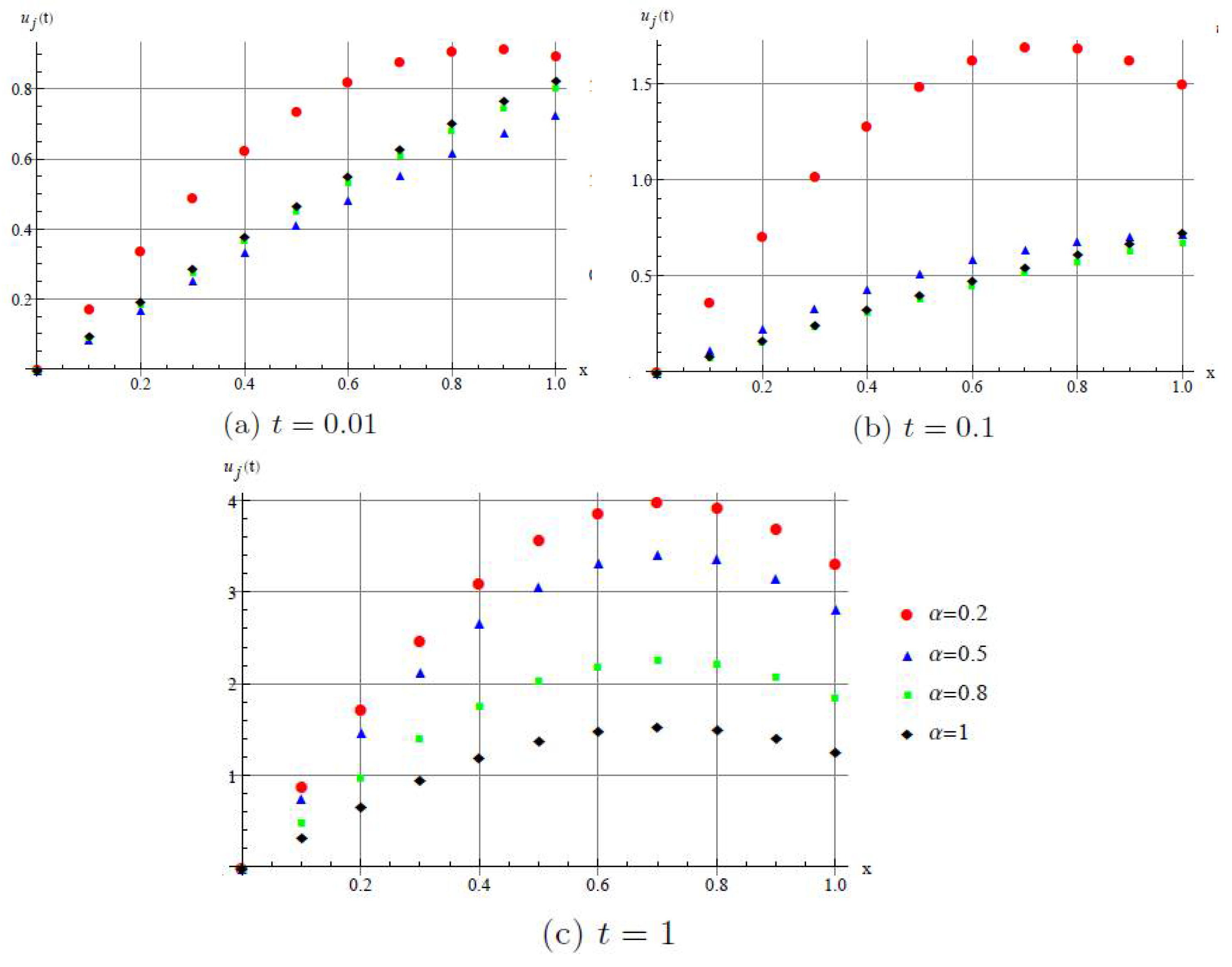
Figure 7 shows the DHAM approximate solution of for different values of .
We can see that the different behaviors of the discrete fractional Burgers’ equations for different fractional parameters.
4. Discussion and Conclusions
In this paper, the discrete HAM is successfully applied to find the solutions of linear and nonlinear fractional partial differential equations with time derivative . In contrast to all other analytic methods, it provides us with a simple way to adjust and convergence region of solution series by introducing an auxiliary parameter . This is an obvious advantage of the DHAM. We can simply choose the fractional operator as the auxiliary linear operator. In this way, we obtained solutions in power series. Also we obtained the exact solutions in special case for some equations. However, it is well-known that a power series often has a small convergence radius. The results of test problems show that the DHAM is effective and reliable. It may also be a promising method to solve other nonlinear partial differential equations.
Funding
This research received no external funding.
Acknowledgments
The author would like to thank the reviewers for their valuable comments and suggestions to improve this paper.
Conflicts of Interest
The author declares no conflict of interest.
References
- Ablowitz, M.J.; Clarkson, P.A. Solutions Nonlinear Evolution Equations and Inverse Scattering; Cambridge University Press: New York, NY, USA, 1991. [Google Scholar]
- Herrmann, R. Fractional Calculus—An Introduction for Physicists; World Scientific: Singapore, 2011. [Google Scholar]
- Luchko, Y. Fractional Schrödinger equation for a particle moving in a potential well. J. Math. Phys. 2013, 54, 012111. [Google Scholar] [CrossRef]
- Mickens, R.E. Nonstandard Finite Difference Models of Differential Equations; World Scientific: Singapore, 1994. [Google Scholar]
- Onorato, M.; Osborne, A.R.; Serio, M.; Bertone, S. Freak waves in random oceanic sea states. Phys. Rev. Lett. 2012, 86, 5831–5834. [Google Scholar] [CrossRef] [PubMed]
- Samko, S.G.; Kilbas, A.A.; Marichev, O.I. Fractional Integrals and Derivatives, Theory and Applications; Gordon and Breach: Amsterdam, The Netherlands, 1993. [Google Scholar]
- Babiarz, A.; Niezabitowski, M. Controllability Problem of Fractional Neutral Systems: A Survey. Math. Probl. Eng. 2017, 2017, 4715861. [Google Scholar] [CrossRef]
- Babiarz, A.; Łȩgowski, A.; Niezabitowski, M. Robot Path Control with Al-Alaoui Rule for Fractional Calculus Discretization. In Theory and Applications of Non-Integer Order Systems; Lecture Notes in Electrical Engineering; Babiarz, A., Czornik, A., Klamka, J., Niezabitowski, M., Eds.; Springer: Cham, Switzerland, 2017; Volume 407. [Google Scholar]
- Bayin, S.Ş. On the consistency of the solutions of the space fractional Schrodinger equation. J. Math. Phys. 2012, 53, 042105. [Google Scholar] [CrossRef]
- El-Nabulsi, R.A.; Torres, D.F.M. Fractional action-like variational approach. J. Math. Phys. 2008, 49, 053521. [Google Scholar] [CrossRef]
- El-Nabulsi, R.A. Fractional calculus of variations from extended Erdelyi-Kober operator. Int. J. Mod. Phys B. 2009, 23, 3349–3361. [Google Scholar] [CrossRef]
- El-Nabulsi, R.A. Fractional variational problems from extended exponentially fractional integral. Appl. Math. Comp. 2011, 217, 9492–9496. [Google Scholar]
- Herrmann, R. The fractional Schrodinger equation and the infinite potential well—Numerical results using the Riesz derivative. Gam. Ori. Chron. Phys. 2013, 1, 1–12. [Google Scholar]
- Luchko, Y.; Gorenflo, R. An operational method for solving fractional differential equations with the Caputo derivative. Acta Math. Vietnam. 1999, 24, 207–233. [Google Scholar]
- Malinowska, A.B.; Torres, D.F.M. Introduction to the Fractional Calculus of Variations; Imperial College Press: London, UK, 2012. [Google Scholar]
- Ubriaco, M.R. Entropies based on fractional calculus. Phys. Lett. A 2009, 373, 2516–2519. [Google Scholar] [CrossRef]
- Das, S.; Vishal, K.; Gupta, P.K.; Saha Ray, S. Homotopy analysis method for solving fractional diffusion equation. Int. J. Appl. Math. Mech. 2011, 7, 28–37. [Google Scholar]
- Dehghan, M.; Manafian, J.; Saadatmandi, A. The solution of the linear fractional partial differential equations using the homotopy analysis method. Z. Naturforsch. 2010, 65, 935–949. [Google Scholar]
- Dehghan, M.; Manafian, J.; Saadatmandi, A. Solving nonlinear fractional partial differential equations using the homotopy analysis method. Numer. Methods Part. Differ. Equ. 2010, 26, 448–479. [Google Scholar] [CrossRef]
- Kivshar, Y.S.; Agarwal, G.P. Optical Solitons: From Fibers to Photonic Crystals; Academic Press: San Diego, CA, USA, 2003. [Google Scholar]
- Liao, S.J. The Proposed Homotopy Analysis Technique for the Solution of Nonlinear Problems. Ph.D. Thesis, Shanghai Jiao Tong University, Shanghai, China, 1992. [Google Scholar]
- Scott, A. Nonlinear Science: Emergence & Dynamics of Coherent Structures; Oxford University Press: Oxford, UK, 1999. [Google Scholar]
- Gepreel, K.A. The homotopy perturbation method applied to the nonlinear fractional Kolmogorov-Petrovskii-Piskunov equations. Appl. Math. Lett. 2011, 24, 1428–1434. [Google Scholar] [CrossRef]
- He, J.H. Homotopy perturbation method: A new nonlinear analytic technique. Appl. Math. Comput. 2003, 135, 73–79. [Google Scholar] [CrossRef]
- He, J.H. An elementary introduction to the homotopy perturbation method. Comput. Math. Appl. 2009, 57, 410–412. [Google Scholar] [CrossRef]
- Sezer, A.S.; Yıldırım, A.; Mohyud-Din, S.T. He’s homotopy perturbation method for solving the fractional KdV-Burgers-Kuramoto equation. Int. J. Numer. Method Heat Fluid Flow 2011, 21, 448–458. [Google Scholar] [CrossRef]
- Ahmad, J.; Mohyud-Din, S.T. Solving fractional vibrational problem using restarted fractional Adomian’s decomposition method. Life Sci. J. 2013, 10, 210–216. [Google Scholar]
- Daftardar-Gejji, V.; Jafari, H. Solving a multi-order fractional differential equation using Adomian decomposition method. Appl. Math. Comput. 2007, 189, 541–548. [Google Scholar]
- Daftardar-Gejji, V.; Bhalekar, S. Solving a multi-term linear and non-linear diffusion wave equations of fractional order by Adomian decomposition method. Appl. Math. Comput. 2008, 202, 113–120. [Google Scholar] [CrossRef]
- Dehghan, M.; Abbaszadeh, M.; Mohebbi, A. An implicit RBF meshless approach for solving time fractional nonlinear Sine-Gordon and Klein-Gordon equation. Eng. Anal. Bound. Elem. 2015, 50, 412–434. [Google Scholar] [CrossRef]
- Miller, K.S.; Ross, B. An Introduction to the Fractional Calculus and Fractional Differential Equations; Wiley: New York, NY, USA, 1993. [Google Scholar]
- Mohebbi, A.; Abbaszadeh, M.; Denghan, M. The use of a meshless technique based on collocation and radial basis functions for solving the time fractional Schrödinger equation arising in quantum mechanics. Eng. Anal. Bound. Elem. 2013, 37, 475–485. [Google Scholar] [CrossRef]
- Shirzadi, A.; Ling, L.; Abbasbandy, S. Meshless simulations of the two dimensional fractional-time convection-diffusion-reaction equations. Eng. Anal. Bound. Elem. 2012, 38, 1522–1527. [Google Scholar] [CrossRef]
- Dehghan, M.; Safarpoor, M. The dual reciprocity boundary elements method for the linear and nonlinear two-dimensional time-fractional partial differential equations. Math. Methods Appl. Sci. 2016, 39, 3979–3995. [Google Scholar] [CrossRef]
- Podlubny, I. Fractional Differential Equations; Academic Press: San Diego, CA, USA, 1999. [Google Scholar]
- Bratsos, A.; Ehrhardt, M.; Famelis, I.T. A Discrete Adomian decomposition method for discrete nonlinear Schrödinger equations. Appl. Math. Comput. 2008, 197, 190–205. [Google Scholar] [CrossRef]
- Zhu, H.; Shu, H.; Ding, M. Numerical solutions of partial differential equations by discrete homotopy analysis method. Appl. Math. Comput. 2010, 216, 3592–3605. [Google Scholar] [CrossRef]
- Lu, Z.; Takeuchi, Y. Global asymptotic behavior in single-species discrete diffusion systems. J. Math. Biol. 1993, 32, 67–77. [Google Scholar] [CrossRef]
- Caputo, M. Linear models of dissipation whose Q is almost independent II. Geophys. J. R. Astron. 1967, 13, 529–539. [Google Scholar] [CrossRef]
- Liao, S.J. Beyond Perturbation: Introduction to Homotopy Analysis Method; Chapman and Hall/CRC Press: Boca Raton, FL, USA, 2003. [Google Scholar]
- Fath, G. Propagation failure of traveling waves in a discrete bistable medium. Physica D 1998, 116, 176–190. [Google Scholar] [CrossRef]
- Prehl, J.; Essex, C.; Hoffmann, K.H. Tsallis relative entropy and anomalous diffusion. Entropy 2012, 14, 701–716. [Google Scholar] [CrossRef]
- Prehl, J.; Boldt, F.; Hoffmann, K.H.; Essex, C. Symmetric fractional diffusion and entropy production. Entropy 2016, 18, 275. [Google Scholar] [CrossRef]
- Eisenberg, H.S.; Silberberg, Y.; Morandotti, R.; Boyd, A.R.; Aitchison, J.S. Discrete Spatial Optical Solitons in Waveguide Arrays. Phys. Rev. Lett. 1998, 81, 3383–3386. [Google Scholar] [CrossRef]
- Efremidis, N.K.; Sears, S.; Christodoulides, D.N.; Fleischer, J.W.; Segev, M. Discrete solitons in photorefractive optically induced photonic lattices. Phys. Rev. E 2002, 66, 046602. [Google Scholar] [CrossRef] [PubMed]
- Gatz, S.; Herrmann, J. Soliton propagation in materials with saturable nonlinearity. J. Opt. Soc. Am. B 1991, 8, 2296–2302. [Google Scholar] [CrossRef]
- Gatz, S.; Herrmann, J. Soliton propagation and soliton collision in doubledoped fibers with a non-Kerr-like nonlinear refractive-index change. Opt. Lett. 1992, 17, 484–486. [Google Scholar] [CrossRef] [PubMed]
Figure 1.
Numerical illustration of approximation solution u(x,t) by discrete homotopy analysis method (DHAM). (a) For t = 0.01; (b) For t = 0.1.
Figure 1.
Numerical illustration of approximation solution u(x,t) by discrete homotopy analysis method (DHAM). (a) For t = 0.01; (b) For t = 0.1.


Figure 2.
Comparison with numerical solution of u(x,t) by DHAM and the exact solution when . (a) For t = 0.5; (b) For t = 1; (c) For t = 2.
Figure 2.
Comparison with numerical solution of u(x,t) by DHAM and the exact solution when . (a) For t = 0.5; (b) For t = 1; (c) For t = 2.

Figure 3.
Numerical illustration of imaginary part of approximation solution u(x,t) by DHAM. (a) For t = 0.01; (b) For t = 0.1.
Figure 3.
Numerical illustration of imaginary part of approximation solution u(x,t) by DHAM. (a) For t = 0.01; (b) For t = 0.1.

Figure 4.
Numerical illustration of real part of approximation solution u(x,t) by DHAM. (a) For t = 0.01; (b) For t = 0.1.
Figure 4.
Numerical illustration of real part of approximation solution u(x,t) by DHAM. (a) For t = 0.01; (b) For t = 0.1.

Figure 5.
Comparison with numerical solution of u(x,t) by DHAM and the exact solution when . (a) For t = 0.5; (b) For t = 1; (c) For t = 2.
Figure 5.
Comparison with numerical solution of u(x,t) by DHAM and the exact solution when . (a) For t = 0.5; (b) For t = 1; (c) For t = 2.

Figure 6.
Comparison with numerical solution of u(x,t) by DHAM and the exact solution when . (a) For t = 0.5; (b) For t = 1; (c) For t = 2.
Figure 6.
Comparison with numerical solution of u(x,t) by DHAM and the exact solution when . (a) For t = 0.5; (b) For t = 1; (c) For t = 2.

Figure 7.
Numerical illustration of approximation solution u(x,t) by DHAM. (a) For t = 0.01; (b) For t = 0.1; (c) For t = 1.
Figure 7.
Numerical illustration of approximation solution u(x,t) by DHAM. (a) For t = 0.01; (b) For t = 0.1; (c) For t = 1.

© 2018 by the author. Licensee MDPI, Basel, Switzerland. This article is an open access article distributed under the terms and conditions of the Creative Commons Attribution (CC BY) license (http://creativecommons.org/licenses/by/4.0/).
Share and Cite
MDPI and ACS Style
Özpınar, F. Applying Discrete Homotopy Analysis Method for Solving Fractional Partial Differential Equations. Entropy 2018, 20, 332. https://doi.org/10.3390/e20050332
AMA Style
Özpınar F. Applying Discrete Homotopy Analysis Method for Solving Fractional Partial Differential Equations. Entropy. 2018; 20(5):332. https://doi.org/10.3390/e20050332
Chicago/Turabian StyleÖzpınar, Figen. 2018. "Applying Discrete Homotopy Analysis Method for Solving Fractional Partial Differential Equations" Entropy 20, no. 5: 332. https://doi.org/10.3390/e20050332
Note that from the first issue of 2016, this journal uses article numbers instead of page numbers. See further details here.