Multichannel Signals Reconstruction Based on Tunable Q-Factor Wavelet Transform-Morphological Component Analysis and Sparse Bayesian Iteration for Rotating Machines


Abstract
:1. Introduction
- (1)
- (2)
- convex regularization methods such as the family of L1-norm [14];
- (3)
- (4)
- (1)
- compared to the single-channel signal, the reconstruction of multichannel signals is addressed by the proposed TQWT-MCA and sparse Bayesian iteration method. Meanwhile, the issue of time consumption is improved significantly.
- (2)
- the spatiotemporal relationships among the signals from different channels are considered via the sparse Bayesian iteration algorithm.
- (3)
- the dictionary atom is designed to match the physical structure of periodic impulses caused by the localized fault, thus, the signal distortion problem is addressed effectively.
- (4)
- the periodical impulses-loss problem is addressed via a pre-processing method, i.e., TQWT-MCA technique, in this paper, the periodical impulses can be separated accurately from the external noise and interference components, which means that the periodical impulses and their fault frequencies will be saved.
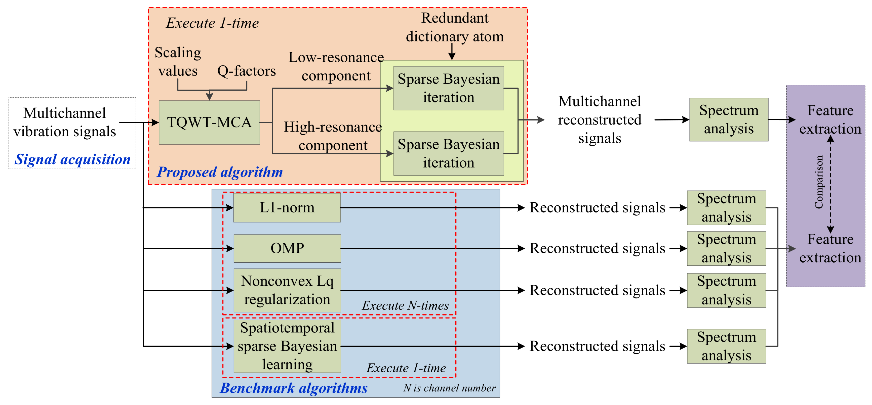
2. TQWT-MCA Algorithm
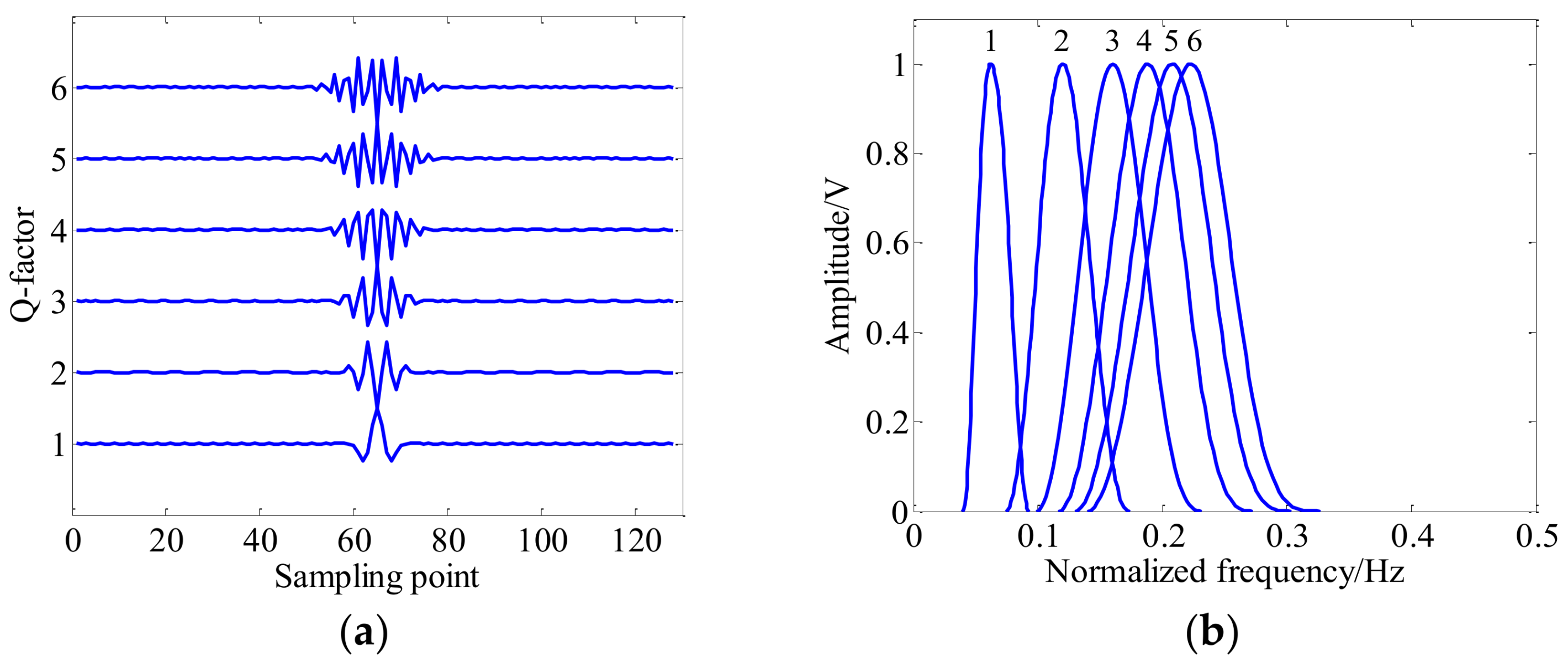
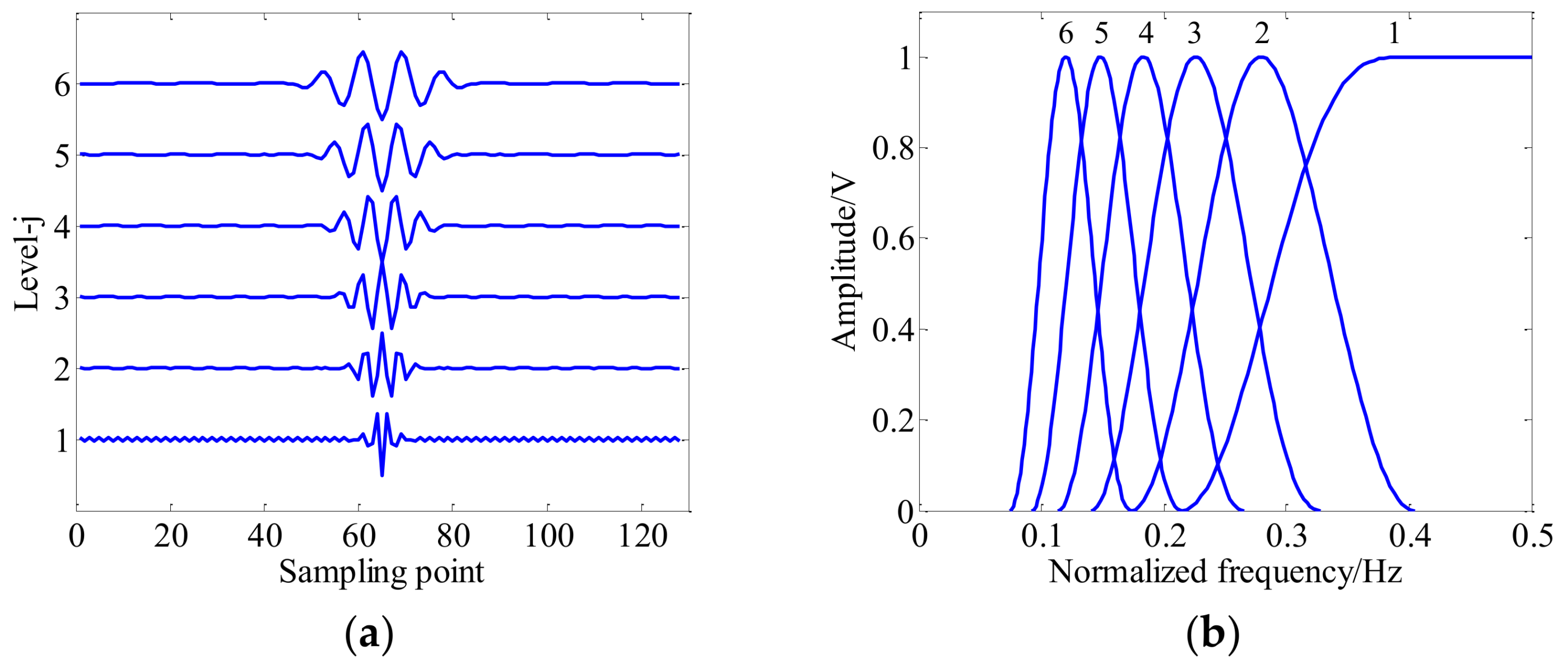
2.1. Tunable Q-Factor Wavelet Transform
2.2. TQWT-Morphological Component Analysis
3. Signal Reconstruction Based on a Sparse Bayesian Iteration Algorithm
3.1. Review of Sparse Bayesian Iteration Framework
3.2. Iteration Rule for Matrix A
3.3. Iteration Rule for Matrix B
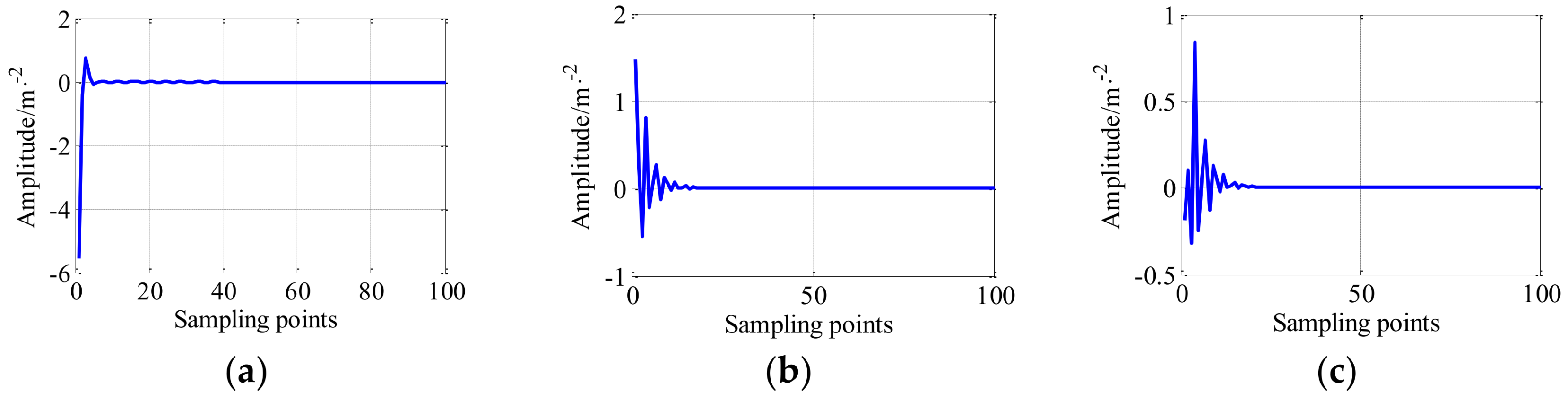
3.4. Redundant Dictionary Atom Based on Step-Impulse Equation
- (1)
- Collect the multichannel raw vibration data of rotating machinery using acceleration sensors;
- (2)
- Chose the appropriate parameters, such as, high-factor Q2 and low-factor Q1 and regularization parameter , etc., according to maximum inner product criterion (MIPC) in Equations (7) and (8). The high-resonance component and low-resonance component can be obtained by TQWT-MCA method;
- (3)
- Establish the redundant dictionary atom based on step-impulse equation in Equations (30)–(32), and then apply the sparse Bayesian iteration to respectively reconstruct the high-resonance component (HRC) and low-resonance component (LRC);
- (4)
- Combined high-resonance component and low-resonance component and obtain the final reconstructed signal;
- (5)
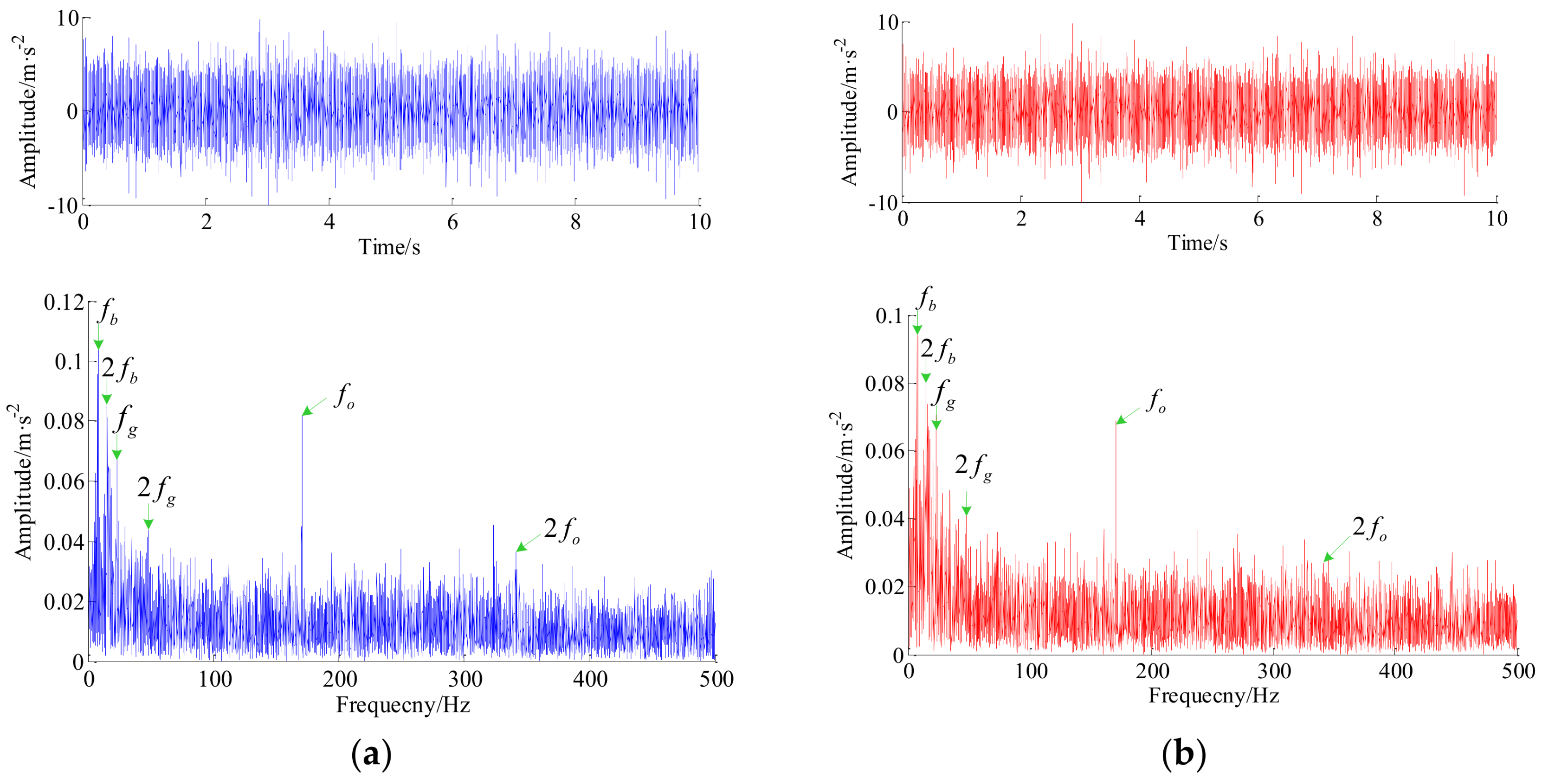
- Detect failure frequency and its harmonics based on the final reconstructed signal;
- (6)
- Comparative analysis with other start-of-the art methods.
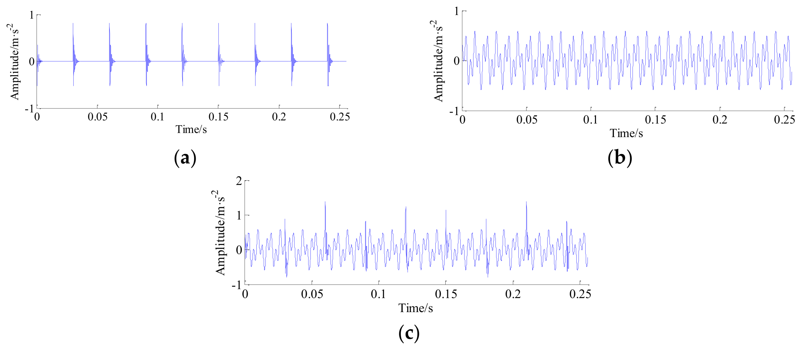
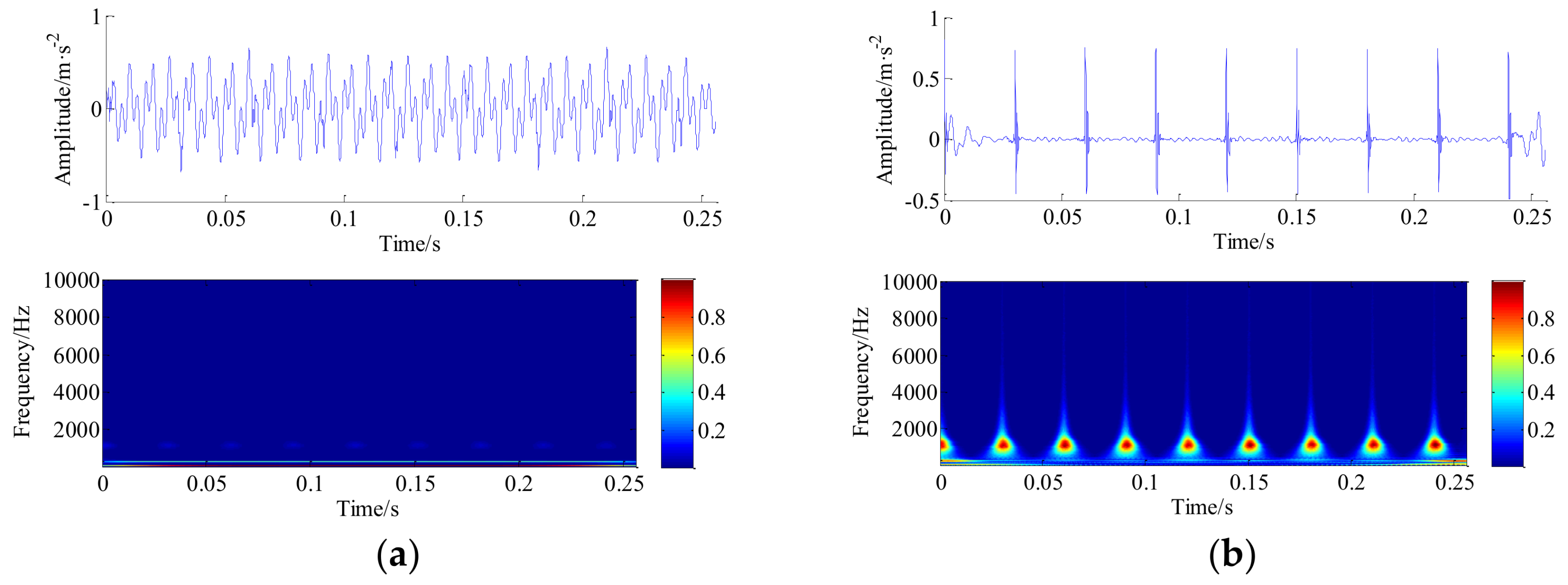
4. Numerical Simulation Case
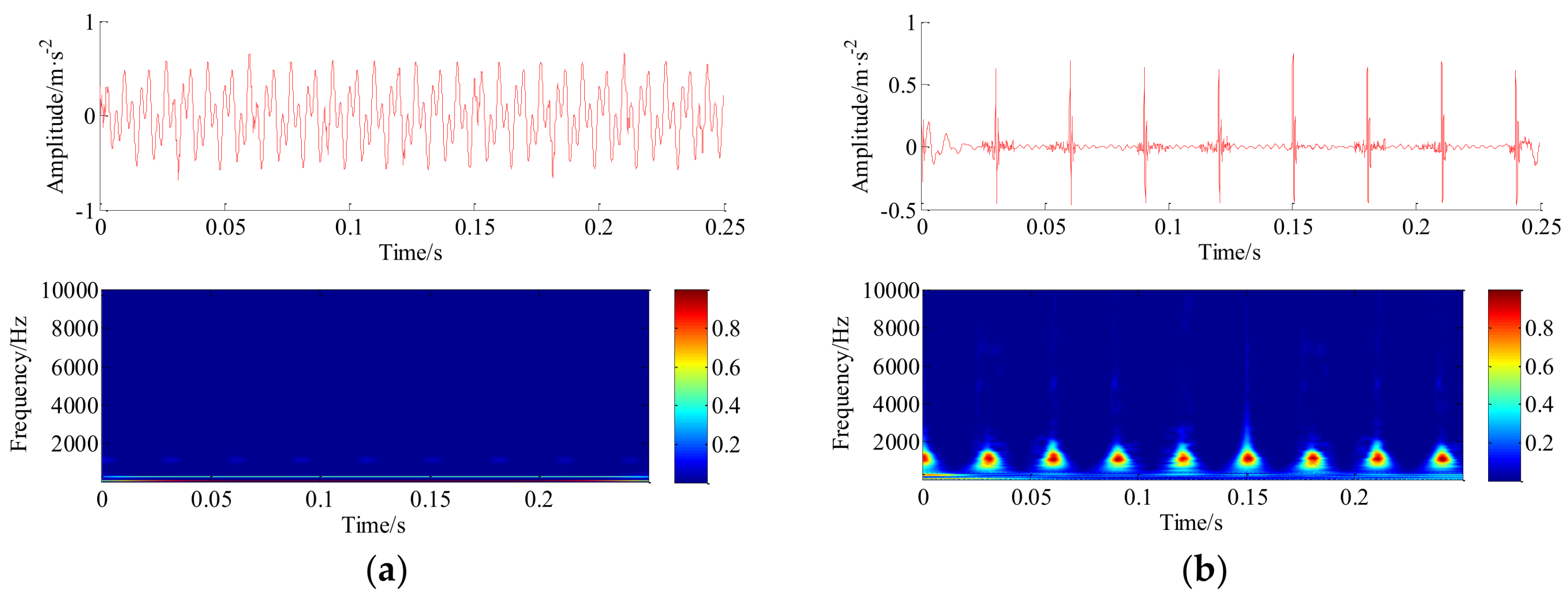
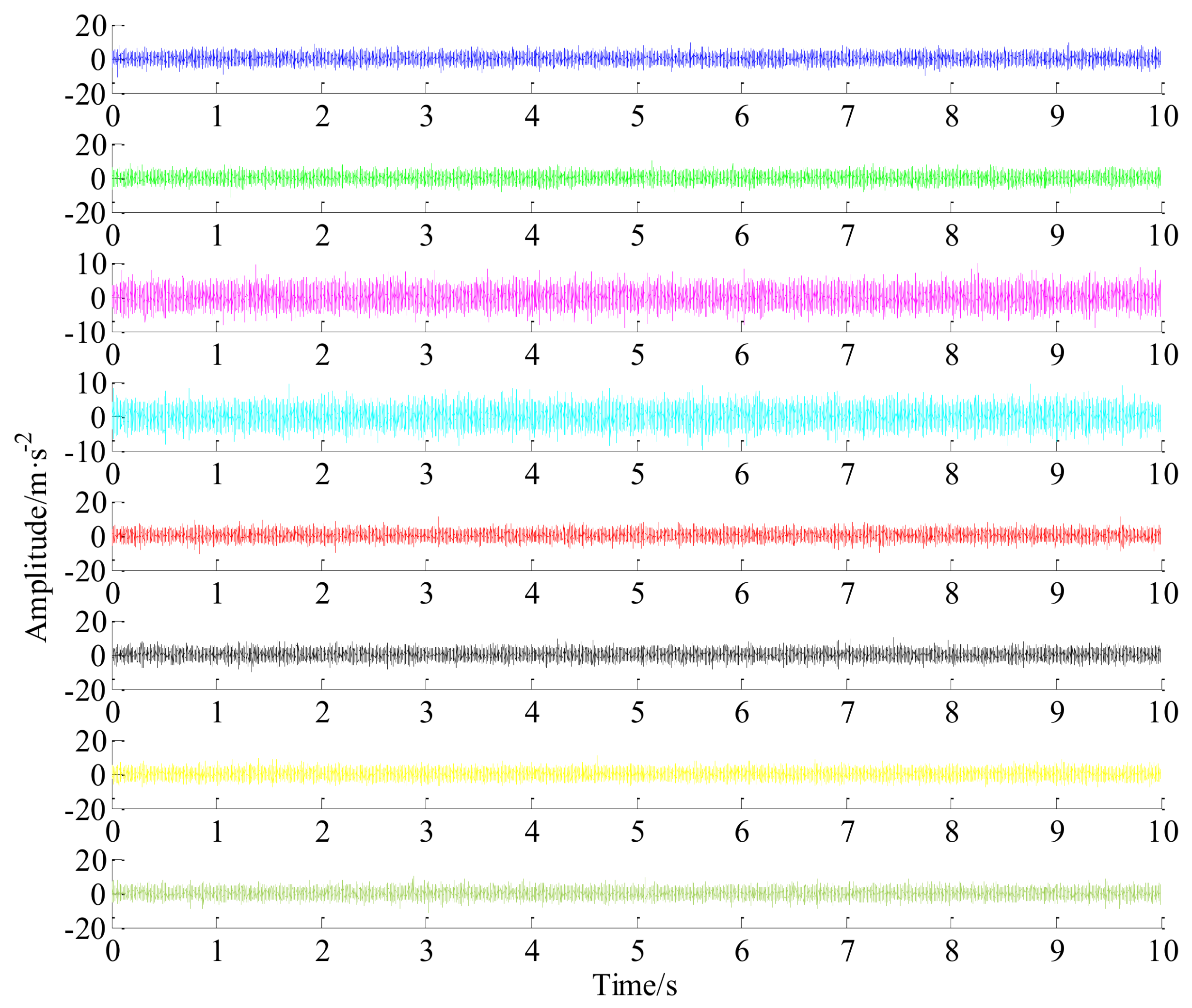
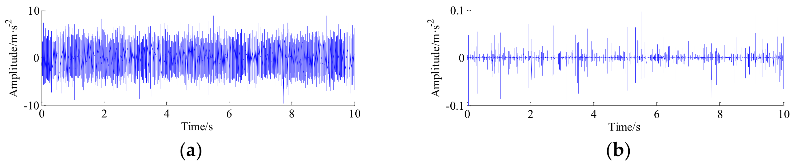
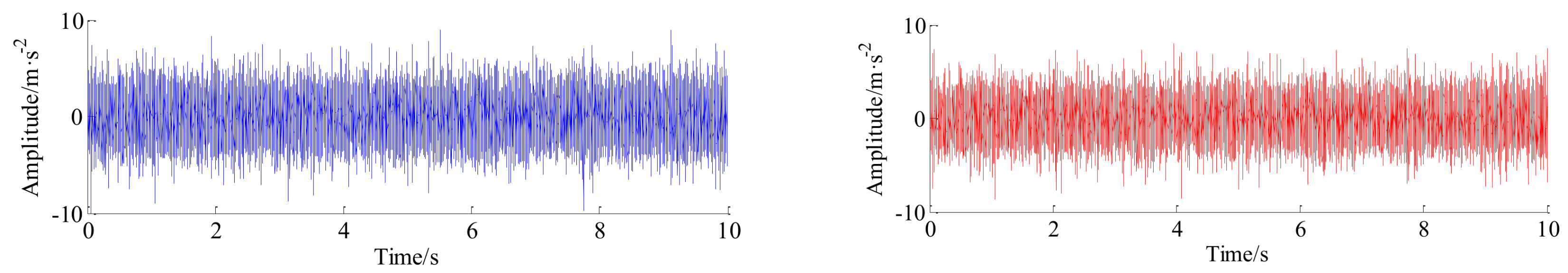
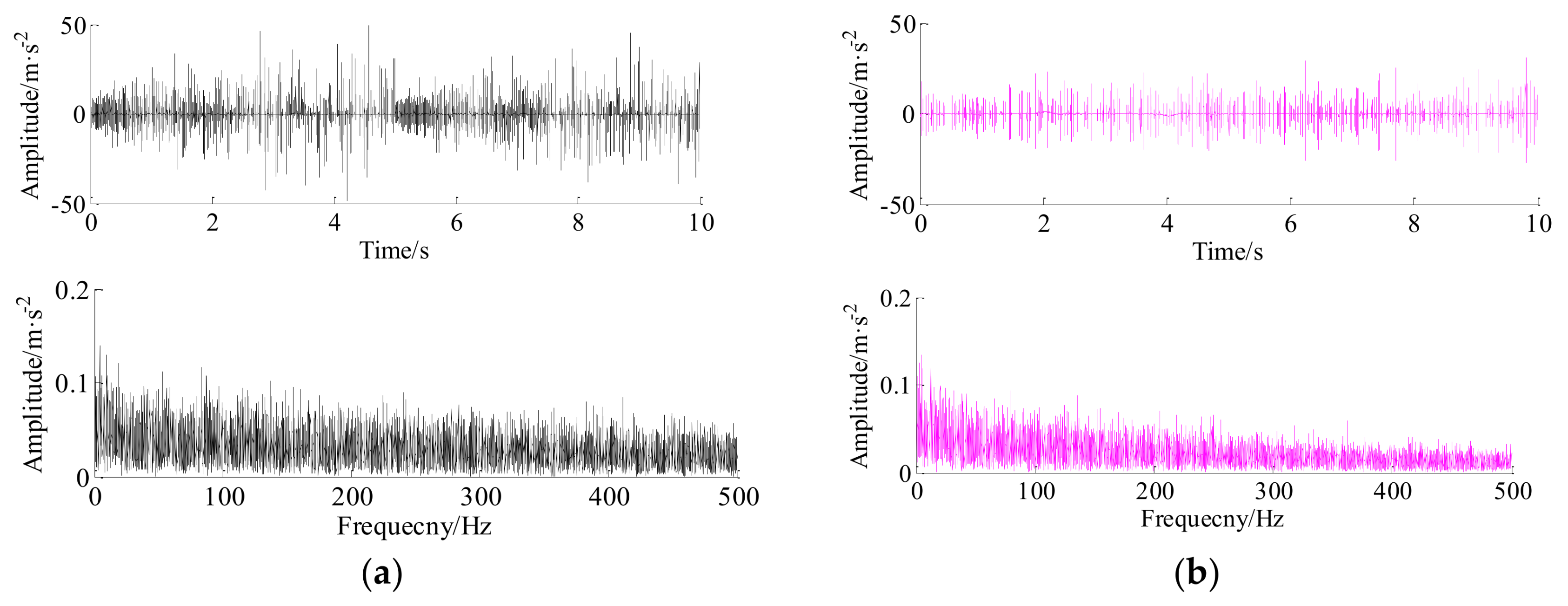
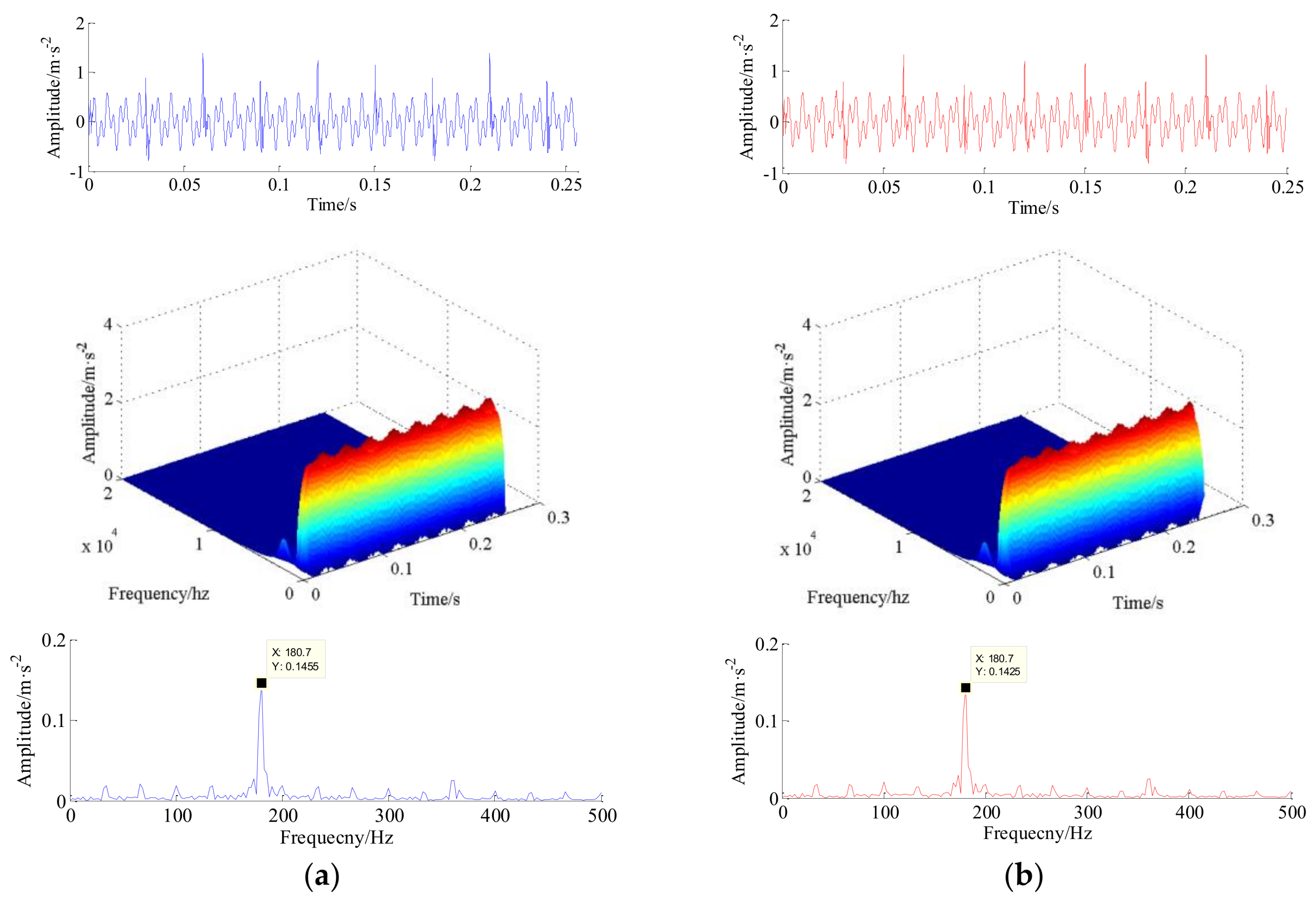
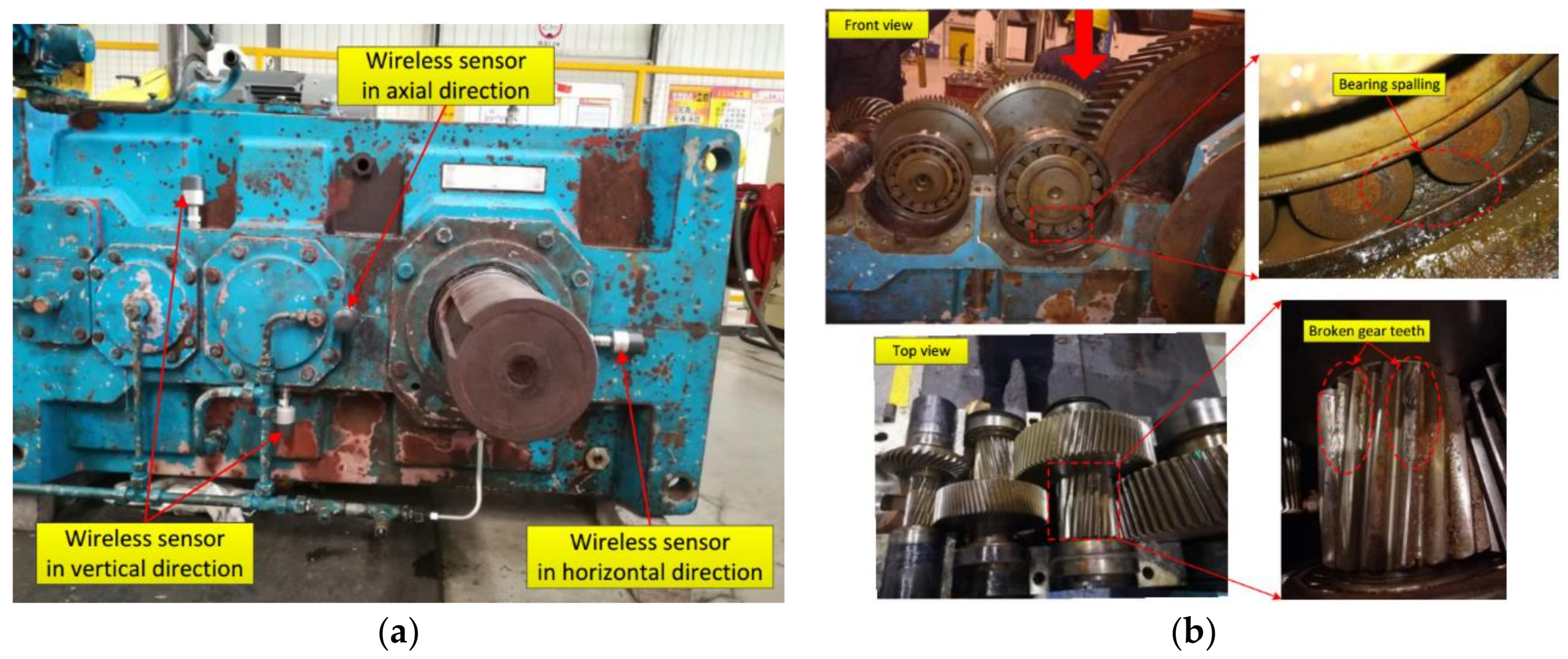
5. Experimental Case and Discussion
6. Conclusions
- (1)
- The raw vibration signal is decomposed into a high-resonance component and low-resonance component, in order to avoid the distortion and aliasing of the periodical impulses when SBL is implemented, and also the periodical impulses caused by the localized fault are preserved. Meanwhile, the dictionary atom is designed to match the physical structure of periodical impulses.
- (2)
- In contrast to existing compressed sensing algorithms, the proposed method not only exploits correlation structures within a single channel signal, but also exploits multiple-channel correlation, which means the spatiotemporal relationships among the signals from different channels are considered via the updating and learning rule of the matrix A and matrix B. The HRC and LRC can be recovered with high accuracy based on the Bayesian iteration algorithm combined with step-impulse dictionary.
- (3)
- Due to it has much better recovery performance than state-of-the-art algorithms, thus, the weak fault information can be immaculately preserved. Meanwhile, the proposed method may relieve the pressure from long-term prognostic and health management in terms of data storage and remote transmission.
Acknowledgments
Author Contributions
Conflicts of Interest
References
- Liu, X.J.; Song, P.; Yang, C.; Hao, C.B.; Peng, W.J. Prognostics and health management of bearings based on logarithmic linear recursive least-squares and recursive maximum likelihood estimation. IEEE Trans. Ind. Electron. 2018, 65, 1549–1558. [Google Scholar] [CrossRef]
- Lall, P.; Lowe, R.; Goebel, K. Prognostics health management of electronic systems under mechanical shock and vibration using Kalman filter models and metrics. IEEE Trans. Ind. Electron. 2012, 59, 4301–4314. [Google Scholar] [CrossRef]
- Kandukuri, S.T.; Klausen, A.; Karimi, H.R.; Robbersmyr, K.G. A review of diagnostics and prognostics of low-speed machinery towards wind turbine farm-level health management. Renew. Sustain. Energy Rev. 2016, 53, 697–708. [Google Scholar] [CrossRef]
- Donoho, D.L. Compressed sensing. IEEE Trans. Inf. Theory 2006, 52, 1289–1306. [Google Scholar] [CrossRef]
- Candés, E.J.; Wakin, M.B. An introduction to compressive sampling. IEEE Signal Process. Mag. 2008, 25, 21–30. [Google Scholar] [CrossRef]
- Lee, S.H.; Lee, Y.H.; Suh, J.S. Accelerating knee MR imaging: Compressed sensing in isotropic three-dimensional fast spin-echo sequence. Magn. Reson. Imaging 2018, 46, 90–97. [Google Scholar] [CrossRef] [PubMed]
- Islam, S.R.; Maity, S.P.; Ray, A.K. Optimal combining fusion on degraded compressed sensing image reconstruction. Signal Process. Image Commun. 2017, 52, 173–182. [Google Scholar] [CrossRef]
- Li, S.L.; Liu, K.; Zhang, F.; Zhang, L.; Xiao, L.L.; Han, D.P. Innovative remote sensing imaging method based on compressed sensing. Opt. Laser Technol. 2014, 63, 83–89. [Google Scholar]
- Saghi, Z.; Divitini, G.; Winter, B.; Leary, R.; Spiecker, E.; Ducati, C.; Midgley, P.A. Compressed sensing electron tomography of needle-shaped biological specimens-Potential for improved reconstruction fidelity with reduced dose. Ultramicroscopy 2016, 160, 230–238. [Google Scholar] [CrossRef] [PubMed]
- Majumdar, A. Causal MRI reconstruction via Kalman prediction and compressed sensing correction. Magn. Reson. Imaging 2017, 39, 64–70. [Google Scholar] [CrossRef] [PubMed]
- Sayed, M.M.A.; Khattab, A.; Elyazeed, M.F.A. RMP: Reduced-set matching pursuit approach for efficient compressed sensing signal reconstruction. J. Adv. Res. 2016, 7, 851–861. [Google Scholar] [CrossRef] [PubMed]
- Zhang, T. Sparse recovery with orthogonal matching pursuit under RIP. IEEE Trans. Inf. Theory 2011, 57, 6215–6221. [Google Scholar] [CrossRef]
- Wang, J.; Shim, B. On the recovery limit of sparse signals using orthogonal matching pursuit. IEEE Trans. Signal Process. 2012, 60, 4973–4976. [Google Scholar] [CrossRef]
- Zhou, L.Y.; Tang, J.X. Fraction-order total variation blind image restoration based on L1-norm. Appl. Math. Model. 2017, 51, 469–476. [Google Scholar] [CrossRef]
- Zhang, Y.J.; Comerford, L.; Kougioumtzoglou, I.A.; Beer, M. Image-norm minimization for stochastic process power spectrum estimation subject to incomplete data. Mech. Syst. Signal Process. 2018, 101, 361–376. [Google Scholar] [CrossRef]
- Li, Q.; Liang, S.Y. Incipient fault diagnosis of rolling bearings based on impulse-step impact dictionary and re-weighted minimizing nonconvex penalty Lq regular technique. Entropy 2017, 19, 421. [Google Scholar] [CrossRef]
- Selesnick, I.W.; Bayram, I. Enhanced sparsity by non-separable regularization. IEEE Trans. Signal Process. 2016, 64, 2298–2313. [Google Scholar] [CrossRef]
- Selesnick, I.W.; Farshchian, M. Sparse signal approximation via non-separable regularization. IEEE Trans. Signal Process. 2017, 65, 2561–2575. [Google Scholar] [CrossRef]
- Parekh, A.; Selesnick, I.W. Improved sparse low-rank matrix estimation. Signal Process. 2017, 139, 62–69. [Google Scholar] [CrossRef]
- Zhang, Z.L.; Rao, B.D. Extension of SBL algorithms for the recovery of block sparse signals with intra-block correlation. IEEE Trans. Signal Process. 2013, 61, 2009–2015. [Google Scholar] [CrossRef]
- Zhang, Z.L.; Rao, B.D. Sparse signal recovery with temporally correlated source vectors using sparse Bayesian learning. IEEE J. Sel. Top. Signal Process. 2011, 5, 912–926. [Google Scholar] [CrossRef]
- Zhang, Z.L.; Jung, T.P.; Makeig, S.; Pi, Z.Y.; Rao, B.D. Spatiotemporal sparse Bayesian learning with applications to compressed sensing of multichannel physiological signals. IEEE Trans. Neural Syst. Rehabil. Eng. 2014, 22, 1186–1197. [Google Scholar] [CrossRef] [PubMed]
- Li, Q.; Ji, X.; Liang, S.Y. Incipient fault feature extraction for rotating machinery based on improved AR-minimum entropy deconvolution combined with Variational mode decomposition approach. Entropy 2017, 19, 317. [Google Scholar] [CrossRef]
- Xu, X.Q.; Zhao, M.; Lin, J.; Lei, Y.G. Envelope harmonic-to-noise ratio for periodic impulses detection and its application to bearing diagnosis. Measurement 2016, 91, 385–397. [Google Scholar] [CrossRef]
- Chen, J.L.; Pan, J.; Zhang, C.L.; Luo, X.Y.; Zhou, Z.T.; Wang, B. Specialization improved nonlocal means to detect periodic impulse feature for generator bearing fault identification. Renew. Energy 2017, 103, 448–467. [Google Scholar] [CrossRef]
- Henao, H.; Capolino, G.A.; Fernandez, C.M.; Filippetti, F.; Bruzzese, C.; Strangas, E.; Pusca, R.; Estima, J.; Riera, G.M.; Hedayati, K.S. Trends in fault diagnosis for electrical machines: A review of diagnostic Techniques. IEEE Ind. Electron. Mag. 2014, 8, 31–42. [Google Scholar] [CrossRef]
- Frosini, L.; Harlisca, C.; Szabo, L. Induction machine bearing fault detection by means of statistical processing of the stray flux measurement. IEEE Trans. Ind. Electron. 2015, 62, 1846–1854. [Google Scholar] [CrossRef]
- Selesnick, I.W. Wavelet transform with tunable Q-factor. IEEE Trans. Signal Process. 2011, 59, 3560–3575. [Google Scholar] [CrossRef]
- Selesnick, I.W. Resonance-based signal decomposition: A new sparsity-enabled signal analysis method. Signal Process. 2011, 91, 2793–2809. [Google Scholar] [CrossRef]
- Tzoreff, E.; Weiss, A.J. Expectation-maximization algorithm for direct position determination. Signal Process. 2017, 133, 32–39. [Google Scholar] [CrossRef]
- Bhadra, A. An expectation-maximization scheme for measurement error models. Stat. Probab. Lett. 2017, 120, 61–68. [Google Scholar] [CrossRef]
- Zhao, K.F.; Lian, H. The expectation-maximization approach for Bayesian quantile regression. Comput. Stat. Data Anal. 2016, 96, 1–11. [Google Scholar] [CrossRef]


| High-Q2 | Low-Q1 | Redundancy Rate r2 | Redundancy Rate r1 | Decomposition Levels j2 |
| 7 | 1 | 3 | 3 | 30 |
| Decomposition Levels j1 | Iteration Times | Regularization Parameters | Regularization Parameters | |
| 8 | 100 |
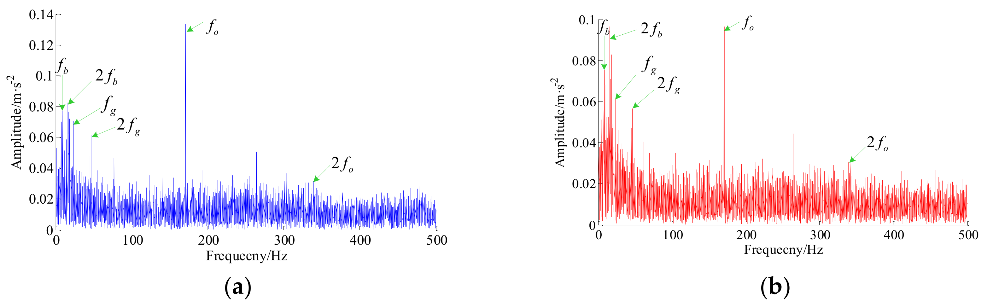
| Bearing Type | Fault Type | Number of Balls | Inner Diameter | Outer Diameter | Outer Race Fault Frequency | Ball Fault Frequency |
|---|---|---|---|---|---|---|
| FAG-32310-A | Outer race | 16 | 50 mm | 110 mm | 170 Hz | 7.4 Hz |
| Axis | Bull Gear | Pinion Gear | Speed Ratio | Rotational Frequency | Meshing Frequency |
|---|---|---|---|---|---|
| Shaft-I | - | 19 | - | 35.233 Hz | 669.433 Hz |
| Shaft-II | 34 | 20 | 0.56 | 19.689 Hz | 393.784 Hz |
| Shaft-III | 81 | 20 | 0.25 | 4.862 Hz | 97.231 Hz |
| Shaft-IV | 81 | 18 | 0.25 | 1.200 Hz | 21.607 Hz |
| Shaft-V | 88 | - | 0.20 | 0.246 Hz |
| High-Q2 | Low-Q1 | Redundancy Rate r2 | Redundancy Rate r1 | Decomposition Levels j2 |
| 7 | 1 | 3 | 3 | 30 |
| Decomposition Levels j1 | Iteration Times | Regularization Parameters | Regularization Parameters | |
| 8 | 100 |
| OMP (s) | Lq-Norm (s) | L1-Norm (s) | SSBL (s) | Proposed Method (s) |
|---|---|---|---|---|
| 98.28 | 952.39 | 228.76 | 3.02 (24.19/8) | 9.08 (72.67/8) |
© 2018 by the authors. Licensee MDPI, Basel, Switzerland. This article is an open access article distributed under the terms and conditions of the Creative Commons Attribution (CC BY) license (http://creativecommons.org/licenses/by/4.0/).
Share and Cite
Li, Q.; Hu, W.; Peng, E.; Liang, S.Y. Multichannel Signals Reconstruction Based on Tunable Q-Factor Wavelet Transform-Morphological Component Analysis and Sparse Bayesian Iteration for Rotating Machines. Entropy 2018, 20, 263. https://doi.org/10.3390/e20040263
Li Q, Hu W, Peng E, Liang SY. Multichannel Signals Reconstruction Based on Tunable Q-Factor Wavelet Transform-Morphological Component Analysis and Sparse Bayesian Iteration for Rotating Machines. Entropy. 2018; 20(4):263. https://doi.org/10.3390/e20040263
Chicago/Turabian StyleLi, Qing, Wei Hu, Erfei Peng, and Steven Y. Liang. 2018. "Multichannel Signals Reconstruction Based on Tunable Q-Factor Wavelet Transform-Morphological Component Analysis and Sparse Bayesian Iteration for Rotating Machines" Entropy 20, no. 4: 263. https://doi.org/10.3390/e20040263