On the Coherence of Probabilistic Relational Formalisms

Escola Politécnica, Universidade de São Paulo, São Paulo 05508-010, Brazil
*
Author to whom correspondence should be addressed.
Entropy 2018, 20(4), 229; https://doi.org/10.3390/e20040229
Submission received: 22 February 2018
/
Revised: 23 March 2018
/
Accepted: 24 March 2018
/
Published: 27 March 2018
(This article belongs to the Special Issue Foundations of Statistics)
Abstract
:There are several formalisms that enhance Bayesian networks by including relations amongst individuals as modeling primitives. For instance, Probabilistic Relational Models (PRMs) use diagrams and relational databases to represent repetitive Bayesian networks, while Relational Bayesian Networks (RBNs) employ first-order probability formulas with the same purpose. We examine the coherence checking problem for those formalisms; that is, the problem of guaranteeing that any grounding of a well-formed set of sentences does produce a valid Bayesian network. This is a novel version of de Finetti’s problem of coherence checking for probabilistic assessments. We show how to reduce the coherence checking problem in relational Bayesian networks to a validity problem in first-order logic augmented with a transitive closure operator and how to combine this logic-based approach with faster, but incomplete algorithms.
1. Introduction
Most statistical models are couched so as to guarantee that they specify a single probability measure. For instance, suppose we have N independent biased coins, so that has probability p for each one of them. Then, the probability of a particular configuration of all coins is exactly , where n is the number of in the configuration. Using de Finetti’s terminology, we can say that the probabilistic assessments and independence assumptions are coherent as they are satisfied by a probability distribution [1]. The study of coherence and its consequences has influenced the foundations of probability and statistics, serving as a subjectivist basis for probability theory [2,3], as a broad prescription for statistical practice [4,5] and generally as a bedrock for decision-making and inference [6,7,8].
In this paper, we examine the coherence checking problem for probabilistic models that enhance Bayesian networks with relations and first-order formulas: more precisely, we introduce techniques that allow one to check whether a given relational Bayesian network, or a given probabilistic relational model is guaranteed to specify a probability distribution. Note that “standard” Bayesian networks are, given some intuitive assumptions, guaranteed to be coherent [9,10,11]. The challenge here is to handle models that enlarge Bayesian networks with significant elements of first-order logic; we do so by resorting to logical inference itself as much as possible. In the remainder of this section, we explain the motivation for this study and the basic terminology concerning it, and at the end of this section, we state our goals and our approach in more detail.
To recap, a Bayesian network consists of a directed acyclic graph, where each node is a random variable, and a joint probability distribution over those variables, such that the distribution and the graph satisfy a Markov condition: each random variable is independent of its non-descendants given its parents. (In a directed acyclic graph, node X is a parent of node Y if there is an edge from X to Y. The set of parents of node X is denoted . Similarly, we define the children of a node, the descendants of a node, and so on.)
If all random variables in a Bayesian network are categorical, then the Markov condition implies a factorization:
where is the projection of on .
Typically, one specifies a Bayesian network by writing down the random variables , drawing the directed acyclic graph, and then settling on probability values , for each , each and each . By following this methodological guideline, one obtains the promised coherence: a unique joint distribution is given by Expression (1).
The following example introduces some useful notation and terminology.
Example 1.
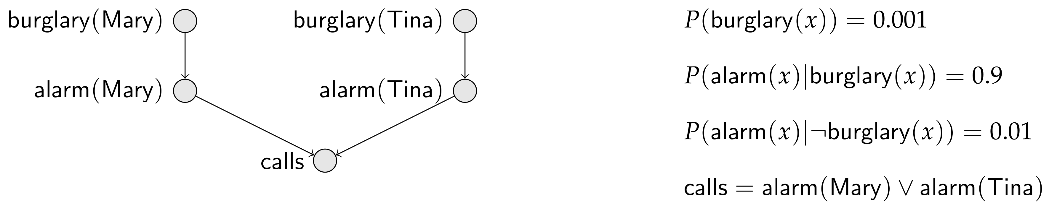
Consider two neighbors, and . The probability that a house is burglarized is in their town. The alarm of a house rings with probability given that the house is burglarized and with probability given the house is not burglarized. Finally, if either alarm rings, the police are called. This little story, completed with some assumptions of independence, is conveyed by the Bayesian network in Figure 1, where means that the house of x (either or ) is burglarized; similarly means that the alarm of x’s house rings; and finally just means that the police are called by someone.
In this paper, every random variable is binary with values zero and one, the former meaning “” and the latter meaning “”. Furthermore, we often write , where X is a random variable, to mean the event , and we often write to mean the event .
Note also that we use, whenever appropriate, logical expressions with random variable names, such as to mean the disjunction of the proposition stating that is and the proposition that is . A random variable name has a dual use as a proposition name.
From the Bayesian network in Figure 1, we compute and .
Here are some interesting scenarios that enhance the previous example:
Example 2.
(Scenario 1) Consider that now we have three people, , and , all neighbors. We can easily imagine an enlarged Bayesian network, with two added nodes related to , and a modified definition where .
(Scenario 2) It is also straightforward to expand our Bayesian network to accommodate n individuals , all neighbors. We may even be interested in reasoning about without any commitments to a fixed n, where is a disjunction over all instances of . For instance, we have that ; hence, the probability of a call to the police will be larger than half for a city with more than 36 inhabitants. No single Bayesian network allows this sort of “aggregate” inference.
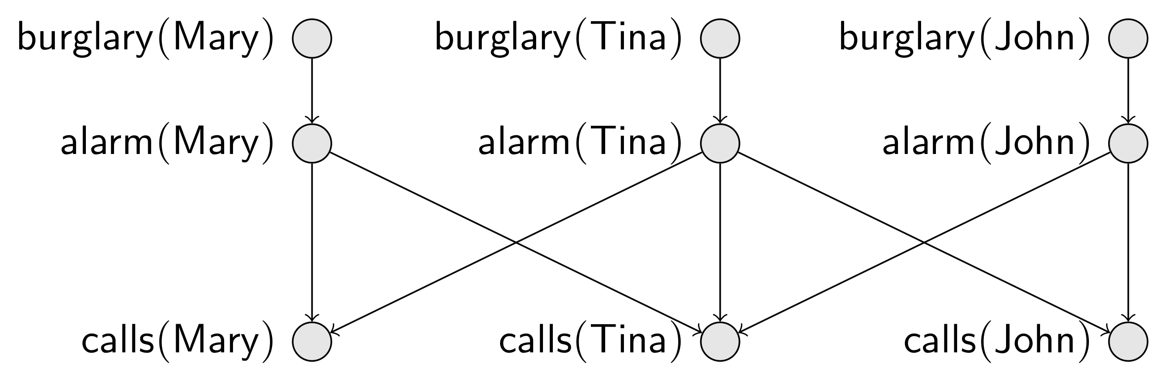
(Scenario 3) Consider a slightly different situation with three people, where: and are neighbors and are neighbors, but and are not neighbors. Suppose also that each person may call the police, depending on neighboring alarms. This new situation is codified into the Bayesian network given in Figure 2.
(Scenario 4) Suppose we want to extend Scenario 3 to a town with n people. Without knowing which pairs are neighbors, there is no way we can predict in advance the structure of the resulting Bayesian network. However, we can reason about the possible networks: for instance, we know that each set of n people produces a valid Bayesian network, without any cycles amongst random variables.
There are many other scenarios where probabilistic modeling must handle repetitive patterns such as the ones described in the previous examples, for instance in social network analysis or in processing data in the semantic web [12,13,14]. The need to handle such “very structured” scenarios has led to varied formalisms that extend Bayesian networks with the help of predicates and quantifiers, relational databases, loops and even recursion [15]. Thus, instead of dealing with a random variable X at a time, we deal with parameterized random variables [16]. We write to refer to a parameterized random variable that yields a random variable for each fixed x in a domain; if we consider individuals a and b in a domain, we obtain random variables and .
Plates offer a popular scheme to manipulate parameterized random variables [17]. A plate is a set of parameterized random variables that share a logical variable, meaning that they are indexed by elements of the same domain. A plate is usually drawn as a rectangle (associated with a domain) containing parameterized random variables. Figure 3 shows simple plate models for the burglary-alarm-call scenario described in Scenario 2 of Example 2.
Plates appeared with the BUGS package, to facilitate the specification of hierarchical models, and have been successful in applications [18]. One restriction of the original plate models in the BUGS package is that a parameterized random variable could not have children outside of its enclosing plate. However, in practice, many plate models violate this restriction. Figure 3 depicts a partial plate model that satisfies the restriction of the original BUGS package (left), and the plate model that violates it (right). Note that as long as the graph consisting of parameterized random variables is acyclic, we know that every Bayesian network generated from the plate model is indeed consistent.
Several other combinations of parameterized random variables and graph-theoretical representations have been proposed, often grouped under the loose term “Probabilistic Relational Model (PRM)” [10,19,20]. Using PRMs, one can associate parameterized random variables with domains, impose constraints on domains and even represent limited forms of recursion [19,21]. A detailed description of PRMs is given in Section 4; for now, it suffices to say that a PRM is specified as a set of “classes” (each class is a set of individuals), where each class is associated with a set of parameterized random variables and additionally by a relational database that gives the relations amongst individuals in classes. The plate model in Figure 3 (left) can be viewed as a diagrammatic representation for a minimalistic PRM, where we have a class containing parameterized random variables. Note that such a minimalistic PRM with a single class cannot encode Scenario 4 in Example 2, as in that scenario, we have pairs of interacting individuals.
Suppose that we want a PRM to represent Scenario 4 in Example 2. Now, the class must include parameterized random variables , and . The challenge is how to indicate which s are parents of a particular . To do so, one possibility is to introduce another class, say , where each element of refers to two elements of . In Section 4 we show how the resulting PRM can be specified textually; for now, we want to point out that finding a diagrammatic representing this PRM is not an obvious matter. Using the scheme suggested by Getoor et al. [19], we might draw the diagram in Figure 4. There, we have a class , a class and a “shadow” class that just indicates the presence of a second in any pair. Dealing with all possible PRMs indeed requires a very complex diagrammatic language, where conditional edges and recursion can be expressed [21].
Instead of resorting to diagrams, one may instead focus just on textual languages to specify repetitive Bayesian networks. A very solid formalism that follows this strategy is Jaeger’s Relational Bayesian Networks (RBNs) [22,23]. In RBNs, relations within domains are specified using a first-order syntax as input, returning an output that can be seen as a typical Bayesian network. For instance, using syntax that will be explained later (Section 2), one can describe Scenario 4 in Example 2 with the following RBN:
- burglary(x) = 0.001;
- alarm(x) = 0.9 * burglary(x) + 0.01 * (1-burglary(x));
- calls(x) = NoisyOR { alarm(y) | y; neighbor(x,y) };
One problem that surfaces when we want to use an expressive formalism, such as RBNs or PRMs, is whether a particular model is guaranteed to always produce consistent Bayesian networks. Consider a simple example [19].
Example 3.
Suppose we are modeling genetic relationships using the parameterized random variable , for any person x. Now, the genetic features of x depend on the genetic features of the mother and the father of x. That is, we want to encode:
If y and z are such that and are , then the probability of depends on and .
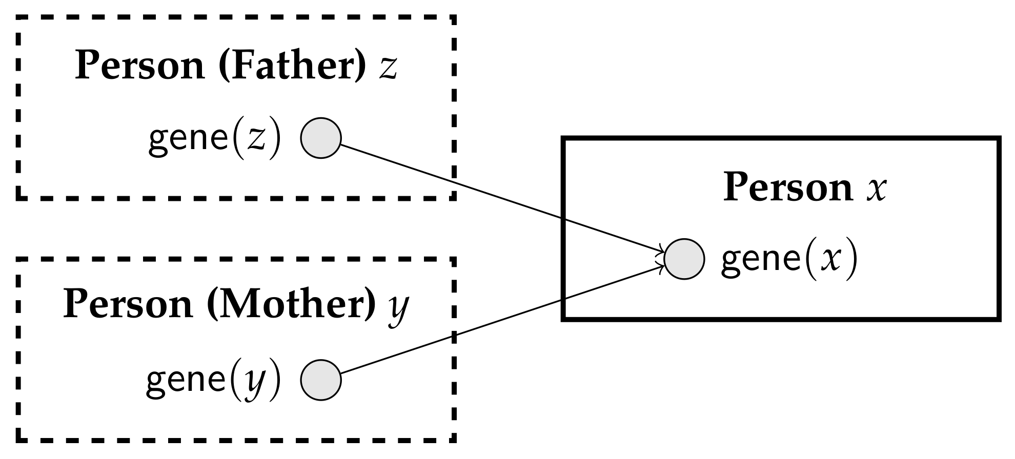
It we try to specify a PRM for this setting, we face a difficulty in that some instances of could depend on other instances of the same parameterized random variable. Indeed, consider drawing a diagram for this PRM, using the conventions suggested by Getoor et al. [19]. We would need a class , containing parameterized random variable , and two shadow classes, one for the father and one for the mother; a fragment of the diagram is depicted in Figure 5. If we could have a that appears as the father of his own father, we would have a cycle in the generated Bayesian network. Of course, we know that such a cycle can never be generated because neither the transitive closure of , nor of can contain a cycle. However, just by looking at the diagram, without any background understanding of and , we cannot determine whether coherence is guaranteed.
The possibility that RBNs and PRMs may lead to cyclic (thus inconsistent) Bayesian networks has been noticed before. Jaeger [23] suggested that checking whether an RBN always produces consistent Bayesian networks, for a given class of domains, should be solved by logical inference, being reducible to deciding the validity of a formula from first-order logic augmented with a transitive closure operator. This path has been explored by De Bona and Cozman [24], yielding theoretical results of very high computational complexity. On a different path, Getoor et al. [19] put forward an incomplete, but more intuitive way of ensuring coherence for their PRMs; in fact, assuming that some sets of input relations never form cycles, one can easily identify a few cases where coherence is guaranteed.
Thus, we have arrived at the problems of interest in this paper: Suppose we have an RBN or a PRM. Is it coherent in the sense that it can be always satisfied by a probability distribution? Is it coherent in the sense that it always produces a unique probability distribution? Such are the questions we address, by exploring a cross-pollination of ideas described in the previous paragraph. In doing so, we bring logical rigor to the problem of coherence of PRMs and present a practical alternative to identifying coherent RBNs.
After formally introducing relational Bayesian networks in Section 2, we review, in Section 3, how its coherence problem can be encoded in first-order logic by employing a transitive closure operator. Section 4 presents PRMs and the standard graph-based approach to their coherence checking. The logical methods developed for the coherence problem of RBNs are adapted to PRMs in Section 5. Conversely, in Section 6, we adapt the graph techniques presented for tackling the coherence of PRMs to the formalism of RBNs.
2. Relational Bayesian Networks
In this section, we briefly introduce the formalism of Relational Bayesian Networks (RBNs). We use the version of RBNs presented in [23], as that reference contains a thorough exposition of the topic.
Let S and R be disjoint sets of relation symbols, called the predefined relations and probabilistic relations, respectively. We assume that S contains the equality symbol =, to be interpreted in the usual way. Each predicate symbol is associated with a positive integer k, which is its arity. Given a finite domain , if V is a set of relation symbols (as R or S), a V-structure is an interpretation of the symbols in V into sets of tuples in D. Formally, a V-structure maps each relation symbol with arity k into a subset of . We denote by the set of all V-structures over a given finite domain D. Given a domain D, a with arity k and a tuple , is said to be a ground V-atom. A V-structure defines truth values for ground atoms: if v is mapped to a relation containing t, we say that is satisfied by , which is denoted by .
Employing the syntax of function-free first-order logic, we can construct formulas using a vocabulary of relations V, together with variables, quantifiers and Boolean connectives. We call these V-formulas, and their meaning is given by the first-order logic semantics, as usual, through the V-structures. We denote by a V-formula where are free variables, in the usual sense. If is a V-formula and is a V-structure, denotes that is satisfied by .
A random relational structure model for S and R is a partial function P that takes an S-structure , over some finite domain D, and returns a probability distribution over the R-structures on the same domain. As an R-structure can be seen as total assignment over the ground R-atoms, can be seen as a joint probability distribution over these ground atoms. An example of random relational structure model would be a function in Scenario 4 of Example 2 that receives an S-structure of neighbors and returns a joint probability distribution over ground atoms for , , . In that scenario, a given configuration of neighbors, over a given domain D, implies a specific Bayesian network whose variables are the ground atoms for , , , which encodes a joint probability distribution, , over these variables. If is the configuration of neighbors from Scenario 4 of Example 2, would be captured by the Bayesian network in Figure 2.
Relational Bayesian networks provide a way to compactly represent random relational structure models. This is achieved by mapping each S-structure into a ground Bayesian network that encodes a probability distribution over R-structures. To begin, this ground Bayesian network has nodes representing (ground atoms), for each and , where k is the arity of r. Thus, given the domain D of the input S-structure, the nodes in the corresponding Bayesian network are already determined. To define the arcs and parameters of the Bayesian network associated with an arbitrary S-structure, relational Bayesian networks employ their central notion of probability formula.
Probability formulas are syntactical constructions intended to link the probability of a ground atom to the probabilities of other ground atoms , according to the S-structure. Once an R-structure and an S-structure are fixed, then for elements in the domain D, a probability formula should evaluate to a number in .
The definition of probability formulas makes use of combination functions, which are functions from finite multi-sets over the interval to numbers in the same interval. We use to denote multi-sets. For instance, NoisyOR is a combination function such that, if , NoisyOR.
Definition 1.
Given disjoint sets S and R of relation symbols and a tuple x of k variables, is a (S,R)-probability formula if:
- (constants) for a ;
- (indicator functions) for an with arity k;
- (convex combinations) , where are probability formulas, or;
- (combination functions) , where is a combination function, are probability formulas, y is a tuple of variables and is an S-formula.
Relational Bayesian networks associate a probability formula to each probabilistic relation , where x is a tuple of k variables, with k the arity of :
Definition 2.
Given disjoint sets of relation symbols S and R, the predefined and probabilistic relations, a relational Bayesian network is a set , where each is a (S,R)-probability formula.
To have an idea of how probability formulas work, consider a fixed S-structure over a domain D. Then, an R-structure over D entails a numeric value for each ground probability formula , denoted by , where t is tuple of elements in D. This is done inductively, by initially defining if , and otherwise, for each , for all . If , then , for any tuple t. The numeric value of for probability formulas that are convex combinations or combination function will require the evaluation of its subformulas , which recursively end at the evaluation of ground atoms or constants c. As the set of ground atoms whose evaluation is needed to compute depends only on the S-structure , and not on , it is denoted by and can be defined recursively:
- ;
- ;
- ;
- is given by:Here, denotes the concatenation of the tuples t and .
For a given S-structure , we can define a dependency relation between the nodes and in the Bayesian network via the probability formulas and by employing the corresponding . Intuitively, contains the ground atoms whose truth value in a structure determines the value of , which is meant to be the probability of . That is, contains the parents of .
Definition 3.
Relation ⪯, over ground R-atoms, is defined as follows:
When this relation is acyclic, a relational Bayesian network defines, for a given S-structure over a finite domain D, a probability distribution over the R-structures over D via:
Example 4.
Scenario 4 of Example 2: We can define a relational Bayesian network that returns the corresponding Bayesian network for each number and configuration of neighbors. Let and . We assume that the relation is reflexive and symmetrical. For each relation in R, we associate a probability formula, forming the relational Bayesian network Φ:
- ; a constant;
- ; a convex combination;
- NoisyOR; a combination function.
Note that, if and are probability formulas, then and are convex combinations and, thus, probability formulas. As the inputs of the NoisyOR above are in , the combination function actually works like a disjunction.
Given an S-structure over a domain D, Φ determines a joint probability distribution over the ground R-atoms, via a Bayesian network. If we take an S-structure over a domain such that , but , the resulting is the model for Scenario 3 in Example 2, whose Bayesian network is given in Figure 2.
3. The Coherence Problem for RBNs
It may happen for a relational Bayesian network that some S-structures yield a cyclic dependency relation ⪯. When the relation ⪯ is cyclic for an S-structure, no probability distribution is defined over the R-structures. In such a case, we say is incoherent for that S-structure. This notion can be generalized to a class of S-structures , so that we say that is coherent for iff the resulting relation ⪯ is acyclic for each S-structure in . To know whether a relational Bayesian network is coherent for a given class of S-structures is precisely one of the problems we are interested in this work.
In order to reason about the relation between a class of S-structures and the coherence of a relational Bayesian network for it, we need to formally represent these concepts. To define a class of S-structures, note that they can be seen as first-order structures over which S-formulas are interpreted. That is, an S-formula defines the set of S-structures satisfying it. If is a closed S-formula (without free variables), we say that is the set of S-structures such that . We denote by an S-formula satisfied exactly by the S-structures in a given class ; that is, .
To encode the coherence of , we need to encode the acyclicity of the dependency relation ⪯ resulting from an S-structure. Ideally, we would like to have a (first-order) S-formula, say , that would be only for S-structures yielding acyclic dependency relations ⪯. If that formula were available, a decision about the coherence of for the class would be reduced to a decision about the validity of the first-order formula : When the formula is valid, then every S-structure in the class guarantees that the resulting dependency relation ⪯ for is acyclic; hence, is coherent for ; otherwise, there is an S-structure in yielding a cyclic dependency relation ⪯ for . Note that for S-formulas, only S-structures matter, and we could ignore any relation not in S. To be precise, if a first-order structure falsifies , then there is an S-structure (formed by ignoring non-S relations) falsifying it.
Alas, to encode cycles in a graph, one needs to encode the notion of path, which is the transitive closure of a relation encoding arcs. It is a well-known fact that first-order logic cannot express transitivity. To circumvent that, we can add a (strict) transitive closure operator to the logic, arriving at the so-called transitive closure logics, as described for instance in [25].
This approach was first proposed by Jaeger [23], who assumed one could write down the S-formula by employing a transitive closure operator. He conjectured that with some restrictions on the arity of the relations in S and R, one could hope to obtain a formula that is decidable. Nevertheless, no hint was provided as to how to construct such a formula, or as to its general shape. A major difficulty is that, if an S-structure satisfying has domain , the size of the resulting Bayesian network is typically greater than n, with one node per ground atom, so a cycle can also contain more nodes than n. There seems to be no direct way of employing the transitive closure operator to devise a formula that encodes cycles with more than n nodes and that is to be satisfied by some structures over a domain with only n elements. In the next sections, we review a technique (introduced by the authors in [24]) to encode for an augmented domain, through an auxiliary formula whose satisfying structures will represent both the S-structure and the resulting ground Bayesian network. Afterwards, we adapt the formula accordingly.
3.1. Encoding the Structure of the Ground Bayesian Network
Our idea to construct a formula , for a given relational Bayesian network , is first to find a first-order V-formula , for some vocabulary V containing S, that is satisfiable only by V-structures that encode both an S-structure and the structure of the ground Bayesian network resulting from it. These V-structures should contain, besides an S-structure , an element for each node in the ground Bayesian network and a relation capturing its arcs. Then, we can use a transitive closure operator to define the existence of paths (and cycles) via arcs, for enforcing acyclicity by negating the existence of a cycle.
Suppose we have two disjoint vocabularies S and of predefined and probabilistic relations, respectively. We use to denote the arity of a relation v. Consider a relational Bayesian network , where each is a (S,R)-probability formula. Let be a V-structure satisfying . We want to be defined over a bipartite domain , where is used to represent an S-structure and is the domain where the structure of the resulting ground Bayesian network is encoded. We overload names by including in V a unary predicate that shall be for all and only the elements in . The structure shall represent the structure of the ground Bayesian network , over the elements of , that is induced by the S-structure codified in . In order to accomplish that, must have an element in for each ground atom over the domain . Furthermore, the V-structure must interpret a relation, say , over according to the arcs of the Bayesian network .
Firstly, we need to define a vocabulary V that includes the predefined relations in S and contains the unary predicate (recall that the equality symbol (=) is included in S). Furthermore, V must contain a binary relation to represent the arcs of the ground Bayesian network. As auxiliary relations for defining , we will need a relation , for each pair , whose arity is . For elements in to represent ground atoms , we use relations to associate elements in to relations r and to tuples . For each relation , we have a unary relation , where is intended to mean that the element represents a ground atom of the form . As for the tuples, recall that each represents an element in the set over which the S-structure is codified. Hence, we insert in V binary relations for every , such that should be iff the element corresponds to a ground atom where , for a and some .
To save notation, we use to denote henceforth, meaning the element x in the domain represents the ground atom , where .
Now, we proceed to list, step-by-step, the set of conjuncts required in , together with their meaning, for the V-structure in to hold the desired properties. To illustrate the construction, each set of conjuncts is followed by an example based on the RBN in Example 4, possibly given in an equivalent form for clarity.
We have to ensure that the elements in correspond exactly to the ground atoms in the ground Bayesian network .
- Each element in should correspond to a ground atom for some . Hence, we have the formula:
- No element may correspond to ground atoms for two different . Therefore, the formula below is introduced:
- Each element corresponding to a ground atom should correspond to exactly one tuple. To achieve that, let , and introduce the formula below:
- Each element corresponding to a ground atom for a should be linked a to tuple with arity . Thus, let , and introduce the formula below for each :
- Only elements in should correspond to ground atoms. This is enforced by the following formula, where :
- Each ground atom must be represented by at least one element (in ). Therefore, for each , with , we need a formula:These formulas enforce that each ground atom is represented by an element x that is in , due to the formula (6).
- No ground atom can be represented by two different elements. Hence, for each , with , we introduce a formula:
The conjunction of all formulas in (2)–(8) is satisfied only by structures over the domain such that there is a bijection between and the set of all possible ground atoms for some and . Now, we can put the arcs over these nodes to complete the structure of the ground Bayesian network .
The binary relation must hold only between elements in the domain D representing ground atoms and such that . Recall that the dependency relation ⪯ is determined by the S-structure . While the ground atoms represented in , for a fixed R, are determined by the size of by itself, the relation between them depends also on the S-formulas that hold for the S-structure . We want these S-structures to be specified by over only, not over . To ensure this, we use the following group of formulas:
- For all , consider the formula below, where :
The formula above forces that , for any , can be only for tuples .
For a known S-structure , it is straightforward to determine which ground atoms are the parents of in the ground Bayesian network . One can use recursively the definition of the set of parents given in Section 2. Nonetheless, with an unknown S-structure specified in over , the situation is a bit trickier. The idea is to construct, for each pair and , an S-formula that is iff for the encoded in . To define , we employ auxiliary formulas , for a ground probability formula and a ground atom , that will be an S-formula that is satisfied by iff . We define recursively, starting from the base cases.
- If , for a , then .
- If , then if ; and otherwise;and .
Above, is a short form for , where k is the arity of t. These base cases are in line with the recursive definition of presented in Section 2. The third case is also straightforward:
- If , then .
In other words, the computation of depends on , for some , if the computation of some , for , depends on .
The more elaborated case happens when is a combination function, for which there is an S-formula involved. Recall that if , then the parents of are given by . Thus, to recursively define , we need an S-formula that is satisfied by an S-structure iff:
The inner union is analogous to the definition of for convex combinations. However, to cope with any such that , we need an existential quantification:
- If , then we have that:
Now, we can employ the formulas to define the truth value of the ground relation , that codifies when .
- For each pair , with and , we have the formula:
In the formula above, has free variables and is built according to the four recursive rules that define , replacing the tuples t and by x and y. We point out that such construction depends only on probability formulas in the relational Bayesian network , and not on any S-structure. To build each , one just starts from the probability formula and follows the recursion rules until reaching the base cases, when will be formed by subformulas like , S-formulas and equalities , possibly quantified on variables appearing in .
The relation is defined now over elements that represent ground atoms and such that , meaning that . This can be achieved in two parts: ensuring that each implies ; and guaranteeing that is true only if for a pair of relations .
- For each pair , with and , let y and denote and , respectively:
- Let be the maximum arity in R, and let y and y denote the tuples and , respectively:
Definition 4.
For some fixed relational Bayesian networks , the formula is satisfied only by V-structures over a bipartite domain such that:
- the relations in S are interpreted in , forming an S-structure ;
- there is a bijection b between the domain and set of all ground R-atoms formed by the tuples in ;
- each is linked exactly to one , via the predicate , and exactly elements in , via the relations , and no ground atom is represented through these links twice;
- the relation is interpreted as arcs in in such a way that form a directed graph that is the structure of the ground Bayesian network .
3.2. Encoding Coherence via Acyclicity
The original formula was intended to capture the coherence of the relational Bayesian network . Our idea is to check the coherence by looking for cycles in the ground Bayesian network encoded in any V-structure satisfying . Hence, we replace by an implication , which is to be satisfied only by V-structures such that, if represents an S-structure and the resulting ground Bayesian network , then is acyclic. Thus, should avoid cycles of the relation in the V-structures satisfying it.
There is a cycle with -arcs in a V-structure over a domain D iff there exists a such that there is a path of -arcs from x to itself. Consequently, detecting -cycles reduces to computing -paths or -reachability. We say y is -reachable from x, in a V-structure , if there are such that , , and . Thus, for each k, we can define reachability through k -arcs: . Unfortunately, the size of the path (k) is unbounded a priori, as the domain D can be arbitrarily large. Therefore, there is no means in the first-order logic language to encode reachability, via arbitrarily large paths, with a finite number of formulas. In order to circumvent this situation, we can resort to a transitive closure logic.
Transitive closure logics enhance first-order logics with a transitive closure operator that we assume to be strict [25]. If is a first-order formula, means that y is -reachable from x, with a non-empty path. Accordingly, a V-structure , over a domain D, satisfies iff there is a and there are such that , and .
Employing the transitive closure operator, the existence of a -path from a node x to itself (a cycle) is encoded directly by ; similarly, the absence of a -cycle is enforced by .
At this point, the V-structures over a domain D satisfying have the following format:
- either it encodes an S-structure in (the part of the domain satisfying ) and the corresponding acyclic ground Bayesian network in .
- or it is not the case that encodes both an S-structure in and the corresponding ground Bayesian network in ;
Back to the coherence-checking problem, we need to decide, for a fixed relational Bayesian network , whether or not a given class of S-structures ensures the acyclicity of the resulting ground Bayesian network . Recall that the class must be defined via a (first-order) S-formula . As we are already employing the transitive closure operator in , we can also allow its use in , which is useful to express S-structures without cycles, for instance.
To check the coherence of for a class , we cannot just check the validity of:
because specifies S-structures over D, while presupposes that the S-structure is given only over . To see the kind of problem that might occur, think of the class of all S-structures where each is such that holds, for some unary predefined relation . Consider an S-structure (), over a domain D. The formula cannot be satisfied by , for must hold for all , because of the formulas in (9), so no can represent ground formulas, due to the formulas in (6), contradicting the restrictions in (7) that require all ground atoms to be represented. Hence, this satisfies without encoding the ground Bayesian network, thus falsifying and satisfying , yielding the satisfaction of Formula (13). Consequently, Formula (13) is valid for this specific class , no matter what the relational Bayesian network looks like. Nonetheless, it is not hard to think of a that is trivially incoherent for any class of S-structures, like , with and , where the probability formula associated with the relation is the indicator function , yielding a cyclic dependency relation ⪯.
In order to address the aforementioned issue, we need to adapt , constructing to represent the class in the extended, bipartite domain . The unary predicate is what delimits the portion of D that is dedicated to define the S-structure. Actually, we can define as the set . Therefore, we must construct a V-formula such that the V-structure satisfies iff the S-structure , formed by and the interpretation of the S relations, satisfies . That is, the S-formulas that hold in an S-structure must hold for the subset of a V-structure defined over the part of its domain that satisfies . This can be performed by inserting guards in the quantifiers inside .
Definition 5.
Given a (closed) S-formula , is the formula resulting from applying the following substitutions to :
- Replace each in by ;
- Replace each in by .
Finally, we can define the formula that encodes the coherence of a relational Bayesian network for a class of S-structures :
Definition 6.
For disjoint sets of relations S and R, a given relational Bayesian network and a class of S-structures defined by , .
Putting all those arguments together, we obtain the translation of the coherence-checking problem to the validity of a formula from the transitive closure logic:
Theorem 1
(De Bona and Cozman [24]). For disjoint sets of relations S and R, a given relational Bayesian network Φ and a class of S-structures defined by , Φ is coherent for iff is valid.
As first-order logic in general is already well-known to be undecidable, adding a transitive closure operator clearly does not make things easier. Nevertheless, decidability remains an open problem, even restricting the relations in R to be unary and assuming a decidable (even though there are some decidable fragments of first-order logic with transitive closure operators [25,26]). Similarly, a proof of general undecidability remains elusive.
3.3. A Weaker Form of Coherence
Jaeger introduced the coherence problem for RBNs as checking whether every input structure in a given class yields a probability distribution via an acyclic ground Bayesian network. Alternatively, we might define the coherence of an RBN as the existence of at least one input structure, out of a given class, resulting in an acyclic ground Bayesian network. This is closer to the satisfiability-like notion of coherence discussed by de Finetti and closer to work on probabilistic logic [27,28].
In this section, we show that, if one is interested in a logical encoding for this type of coherence for RBNs, the transitive closure operator can be dispensed with.
Suppose we have an RBN and class of input structures codified via a first-order formula and we want to decide whether is coherent for some structure in . This problem can be reduced to checking the satisfiability of a first-order formula, using the machinery introduced above, with the bipartite domain. This formula can be easily built as . By construction, this formula is satisfiable iff there is a structure over a bipartite domain where encodes an S-structure in (), encodes the corresponding ground Bayesian network () and the latter is acyclic (). Nonetheless, since now we are interested in satisfiability instead of validity, we can replace by a formula that does not employ the transitive closure operator.
The idea to construct is to use a binary relation and to force it to extend, or to contain, the transitive closure of . The formula then also requires to be irreflexive. If there is such , then must be acyclic. Conversely, if is acyclic, then can be interpreted as its transitive closure, being irreflexive. In other words, we want a structure to satisfy iff it interprets a relation that both is irreflexive and extends the transitive closure of .
In order to build , the vocabulary V is augmented with the binary relation . Now, we can define as the conjunction of two parts:
- , forcing to extend the transitive closure of ;
- , requiring to be irreflexive.
By construction, one can verify the following result:
Theorem 2.
For disjoint sets of relations S and R, a given relational Bayesian network Φ and a class of S-structures defined by , Φ is coherent for some structure in iff is satisfiable.
The fact that does not use the transitive closure operator makes its satisfiability decidable for any decidable fragment of first-order logic.
4. Probabilistic Relational Models
In this section, we introduce the machinery of PRMs by following the terminology by Getoor et al. [19], focusing on the simple case where uncertainty is restricted to descriptive attributes, which are assumed to be binary. We also review the coherence problem for PRMs and the proposed solutions in the literature. In the next section, we show how this coherence problem can also be tackled via logic, as the coherence of RBNs.
4.1. Syntax and Semantics of PRMs
To define a PRM, illustrated in Example 5, we need a relational model, with classes associated with descriptive attributes and reference slots that behave like foreign keys. Intuitively, each object in a class is described by the values of its descriptive attributes, and reference slots link different objects. Formally, a relational schema is described by a set of classes , each of which associated with a set of descriptive attributes and a set of reference slots . We assume descriptive attributes take values in . A reference slot in a class X (denoted ) is a reference to an object of the class (its range type) specified in the schema. The domain type of , , is X. We can view this reference slot as a function taking objects in and returning singletons of objects in . That is, is equivalent to .
For any reference slot , there is an inverse slot such that and . The corresponding function, takes an object x from the class and returns the set of objects from the class . A sequence of slots (inverted or not) is called a slot chain if for all i. The function corresponding to a slot chain , , is a type of composition of the functions , taking an object x from and returning a set objects from . The corresponding function can be obtained by applying this type of composition two-by-two. We write when .
An instance of a relational schema populates the classes with objects, associating values with the descriptive attributes and reference slots. Formally, is an interpretation specifying for each class : a set of objects ; a value for each descriptive attribute in and each object ; and an object for each reference slot and object . Note that, if , . We use and to denote the value of and in .
Given a relational schema, a PRM defines a probability distribution over its instances. In the simplest form, on which we focus, objects and the relations between them are given as input, and there is uncertainty only over the descriptive attributes values. A relational skeleton is a partial specification of an instance that specifies a set of objects for each class in the schema besides the relation holding between these objects: for each and . A completion of a relational skeleton is an instance such that, for each class : and, for each and , . We can see a PRM as a function taking relational skeletons and returning probability distributions over the completions of these partial instances, which can be seen as joint probability distributions for the random variables formed by the descriptive attributes of each object.
The format of a PRM resembles that of a Bayesian network: for each attribute , we have a set of parents and the corresponding parameters . The parent relation forms a direct graph, as usual, called the dependency graph; and the set of parameters define the conditional probability tables. The attributes in are called formal parents, as they will be instantiated for each object x in X according to the relational skeleton. There two types of formal parents: can depend either on another attribute of the same object or on an attribute of other objects, where K is a slot chain.
In general, for an object x, is a multiset , whose size is defined by the relational skeleton. To compactly represent the conditional probability distribution when , the notion of aggregation is used. The attribute will depend on some aggregate function of this multiset, like its mean value, mode, maximum or minimum, and so on; that is, will be a formal parent of .
Definition 7.
A probabilistic Relational model for a relational schema is defined as a pair where:
- defines, for each class and each descriptive attribute , a set of formal parents , where each has the form or ;
- is the set of parameters defining legal Conditional Probability Distributions (CPDs) for each descriptive attribute of each class .
The semantics of a PRM is given by the ground Bayesian network induced by a relational skeleton, where the descriptive attributes of each object are the random variables.
Definition 8.
A PRM and a relational skeleton define a ground Bayesian network where:
- There is a node representing each attribute , for all , and ;
- For each , each and each , there is a node representing for each ;
- Each depends on parents , for formal parents , and on parents , for formal parents , according to ;
- Each depends on parents with ;
- The CPD for is , according to .
- The CPD for is computed through the aggregation function .
The joint probability distribution over the descriptive attributes can be factored as usual to compute the probability of a specific instance that is a completion of the skeleton . If we delete each from the ground Bayesian network, making its children depend directly on the nodes with (defining a new parent relation ) and updating the CPDs accordingly, we can construct a simplified ground Bayesian network. The latter can be employed to factor the joint probability distribution over the descriptive attributes:
Viewing as a function from skeletons to probability distributions over instances, we use to denote the probability distribution over the completions of .
Example 5.
Recall again Scenario 4 in Example 2. We can define a PRM that returns the corresponding Bayesian network for each number and configuration of neighbors. In our relational schema, we have a class , whose set of descriptive attributes is . Furthermore, to capture multiple neighbors, we also need a class , with two reference slots, , whose domain is . For instance, to denote that and are neighbors, we would have an object, say , in the class , whose reference slots would be and .
We assume that the relation is reflexive (that is, for each x, there is always a with ) and symmetrical (if , we also have ).
For each descriptive attribute in our relational schema, we associate a set of formal parents and a conditional probability table, forming the following PRM Π to encode Scenario 4:
- ; ;
- ; and ;
- ;, for .
Given a relational skeleton with persons and neighbors, Π determines a joint probability distribution over the the descriptive attributes, via a Bayesian network. Consider a skeleton with and , with and , for each , but such that no has and . Then, the resulting probability distribution is the model of Scenario 3 in Example 2, whose Bayesian network is given in Figure 2.
4.2. Coherence via Colored Dependency Graphs
As with RBNs, for the model to be coherent, one needs to guarantee that the ground Bayesian network is acyclic. Getoor et al. [19] focused on guaranteeing that a PRM yields acyclic ground Bayesian networks for all possible relational skeletons. To achieve that, possible cycles are detected in the class dependency graph.
Definition 9.
Given a PRM , the class dependency graph is a directed graph with a node for each descriptive attribute and the following arcs:
- Type I arcs: , where is a formal parent of ;
- Type II arcs: , where is a formal parent of and .
When the class dependency graph is acyclic, so is the ground Bayesian network for any relational skeleton. Nevertheless, it may be the case that, even for cyclic class dependency graphs, any relational skeleton occurring in practice leads to a coherent model. In other words, there might be classes of skeletons for which the PRM is coherent. To easily recognize some of these classes, Getoor et al. [19] put forward an approach based on identifying slot chains that are acyclic in practice. A set of slot chains is guaranteed acyclic if we are guaranteed that, for any possible relational skeleton , there is a partial ordering ⪯ over its objects such that, for each , for any pair x and (we use to denote and ).
Definition 10.
Given a PRM and a set of guaranteed acyclic slot chains , the colored class dependency graph is a directed graph with a node for each descriptive attribute and the following arcs:
- Yellow arcs: , where is a formal parent of ;
- Green arcs: , where is a formal parent of , and ;
- Red arcs: , where is a formal parent of , and .
Intuitively, yellow cycles in the colored class dependency graph correspond to attributes of the same object, yielding a cycle in the ground Bayesian network. If we add some green arcs to such a cycle, then it is guaranteed that, departing from a node in the ground Bayesian network, these arcs form a path to , where , since ⪯ is transitive. Hence, x is different from y, and there is no cycle. If there is a red arc in a cycle, however, one may have a skeleton that produces a cycle.
A colored class dependency graph is stratified if every cycle contains at least one green arc and no red arc. Then:
Theorem 3
(Getoor et al. [19]). Given a PRM Π and a set of guaranteed acyclic slot chains , if the colored class dependency graph is stratified, then the ground Bayesian network is acyclic for any possible relational skeleton.
In the result above and in the definition of guaranteed acyclic slot chains, “possible relational skeleton” refers to the class of skeletons that can occur in practice. The user must detect the guaranteed acyclic slot chains, taking advantage of his a priori knowledge on the possible skeletons in practice. For instance, consider a slot chain linking objects of the same class (Example 3). A genetic attribute, like , might depend on . Mathematically, we can conceive of a skeleton with a cyclic relation , resulting in a red cycle in the colored class dependency graph. Nonetheless, being aware of the intended meaning of , we know that such skeletons are not possible in practice, so the cycle is green, and coherence is guaranteed.
Identifying guaranteed acyclic slot chains is by no means trivial. In fact, Getoor et al. [19] also define guaranteed acyclic (g.a.) reference slots and g.a. slot chains are defined as those formed only by g.a. reference slots. Still, these maneuvers miss the cases where two possible reference slots cannot be g.a. according to the same ⪯, but combine to form a g.a. slot chain. Getoor et al. [19] mention the possibility of assuming different partial orders to define different sets of g.a. slot chains: in that case, each ordering would correspond to a shade of green in the colored class dependency graph, and coherence would not be ensured if there were two shades of green in a cycle.
5. Logic-Based Approach to the Coherence of PRMs
The simplest approach to the coherence of PRMs, via the non-colored class dependency graph, is intrinsically incomplete, in the sense that some skeletons might yield a coherent ground Bayesian network even for cyclic graphs. The approach via colored class dependency graph allows some cyclic graphs (the stratified ones) to guarantee consistency for the class of all possible skeletons. However, this method depends on a pre-specified set of guaranteed acyclic slot chains, and the colored class dependency graph being stratified for this set is only a sufficient, not a necessary condition for coherence. Therefore, the colored class dependency graph method is incomplete, as well. Even using different sets of g.a. slot chains (corresponding to shades of green) to eventually capture all of them, it is still possible that a cycle with red arcs cannot entail incoherence in practice. Besides being incomplete, the graph-based method is not easily applicable to an arbitrary class of skeletons. Given a class of skeletons as input, the user would have to detect somehow which slot chains are guaranteed acyclic for that specific class; this can be considerably more difficult than ensuring acyclicity in the general case.
To address these issues, thus obtaining a general, complete method for checking the coherence of PRMs for a given class of skeletons, we can resort to the logic-based approach we introduced for the RBNs in previous sections. The goal of this section is to adapt the logic-basic techniques to PRMs.
PRMs can be viewed as RBNs, as conditional probability tables of the former can be embedded into combination functions of the latter. This translation is out of our scope though, and it suffices for our purposes to represent PRMs as random relational structures, taking S-structures to probability distributions on R-structures. While the S-vocabulary is used to specify classes of objects and relations between them (that is, the relational skeleton), the R-vocabulary expresses the descriptive attributes of the objects. Employing this logical encoding of PRMs, we can apply the approach from Section 3.1 to the coherence problem for PRMs.
To follow this strategy, we first show how a PRM can be seen as a random relational structure described by a logical language.
5.1. PRMs as Random Relational Structures
Consider a PRM over a relational schema described by a set of classes , each associated with a set of descriptive attributes and a set of reference slots . Given a skeleton , which is formed by objects and relations holding between them, the PRM yields a ground Bayesian network over the descriptive attributes of these objects, defining a probability distribution over the completions of . Hence, if the relational skeleton is given as a first-order S-structure over a set of objects and a set of unary relations R denotes their attributes, the PRM becomes a random relational structure.
We need to represent a skeleton as a first-order S-structure . Objects in can be seen as the elements of the domain D of . Note that PRMs are typed, with each object belonging to specific class . Thus, we use unary relations in the vocabulary S to denote the class of each object. Accordingly, for each , holds in iff . As each object belongs to exactly one class in the relational skeleton, the class of possible first-order structures is restricted to those where the relations form a partition of the domain.
The first-order S-structure must also encode the relations holding between the objects in the skeleton that are specified via the values of the reference slots. To capture these, we assume they have unique names and consider, for each reference slot with , a binary relation . In , holds iff . Naturally, should imply and . Now, encodes, through the vocabulary S, all objects of a given class, as well as the relations between them specified in the reference slots. In other words, there is a computable function from relational skeletons to S-structures . For to be a bijection, we make its codomain equal to its range.
The probabilistic vocabulary of the random relational structure corresponding to a PRM is formed by the descriptive attributes of every class in the relational schema. We assume that attributes in different classes have different names, as well, in order to define the vocabulary of unary relations . If is an attribute of , (resp. ) in the PRM is mirrored by the ground R-atom being (resp. ) in the random relational structure. Thus, as a completion corresponds to a value assignment to descriptive attributes of objects from a relational skeleton , it also corresponds to an R-structure over a domain in the following way: iff . Note that we assume that for to correspond to a completion of , whenever is not an attribute of the class such that . Let denote the function taking instances and returning the corresponding R-structures . As we cannot recover the skeleton from the R-structure , is not a bijection. Nevertheless, fixing a skeleton , there is a unique such that .
Now, we can define a random relational structure that corresponds to the PRM . For every relational skeleton over a domain D, let be a probability distribution over R-structures such that , if , for a completion of , and otherwise.
5.2. Encoding the Ground Bayesian Network and its Acyclicity
The probability distribution can be represented by a ground Bayesian network , where nodes represent the ground R-atoms. The structure of this network is isomorphic to the simplified ground Bayesian network yielded by for the skeleton , if we ignore the isolated nodes representing the spurious , when is not an attribute of the class to which belongs. The coherence of depends on the acyclicity of the corresponding ground Bayesian network , which is acyclic iff is so. Therefore, we can encode the coherence of a PRM for a skeleton via the acyclicity of by applying the techniques from Section 3.
We want to construct a formula that is satisfied only by those S-structures such that is coherent. Again, we consider an extended, bipartite domain , with encoded over and the structure of encoded in . We want to build a formula that is satisfied by structures over such that, if encodes over , then encodes the structure of over . The nodes are encoded exactly as shown in Section 3.1.
To encode the arcs, we employ once more a relation . must hold only if denote ground R-atoms and such that in the simplified ground Bayesian network, which is captured by the formula , as in Section 3.1. The only difference here is that now can be defined directly. We use here to denote a formula recursively defined, not an atom over the binary relation . For each pair , we can simply look at to see the conditions on which is a parent of in the simplified ground Bayesian network (), in which case will be a parent of in . If , then should be whenever . If , for a slot chain K, then and should be whenever is related to x via . This is the case if:
is . If , this formula is simply .
Note that it is possible that both and are formal parents of , and there can even be different parents , for different K. Thus, we define algorithmically. Initially, make . If for some , make . Finally, for each in , for a slot chain , make:
using fresh .
Analogously to Section 3.1, we have a formula , for a fixed PRM , that is satisfied only by structures over a bipartite domain where the relation over brings the structure of the ground Bayesian network corresponding to the S-structure encoded in . Again, acyclicity can be captured via a transitive closure operator: . The PRM is coherent for a skeleton if, for every structure over a bipartite domain encoding in , we have .
Consider now a class of skeletons such that is the set of S-structures satisfying a first-order formula . To check whether the PRM is coherent for the class , we construct by inserting guards to the quantifiers, as explained in Definition 5. Finally, the PRM is coherent for a class of relational skeletons iff is valid.
We have thus succeeded in turning coherence checking for PRMs into a logical inference, by adapting techniques we developed for RBNs. In the next section, we travel, in a sense, the reverse route: we show how to adapt the existing graph-based techniques for coherence checking of PRMs to coherence checking of RBNs.
6. Graph-Based Approach to the Coherence of RBNs
The logic-based approach to the coherence problem for RBNs can be applied to an arbitrary class of input structures, as long as the class can be described by a first-order formula, possibly with a transitive closure operator. Given any class of input structures , via the formula , we can verify the coherence of a RBN via the validity of , as explained in Section 3. Furthermore, this method is complete, as is coherent for if and only if such a formula is valid. Nonetheless, completeness and flexibility regarding the input class come at a very high price, as deciding the validity of this first-order formula involving a transitive closure operator may be computationally hard, if at all decidable. Therefore, RBNs users can benefit from the ideas introduced by Getoor et al. [19] for the coherence of PRMs, using the (colored) dependency graphs. While Jaeger [23] proposes to investigate the coherence for a given class of models described by a logical formula, Getoor et al. [19] are interested in a single class of inputs: the skeletons that are possible in practice. With a priori knowledge, the RBN user perhaps can attest to the acyclicity of the resulting ground Bayesian network for all possible inputs.
Any arc in the output ground Bayesian network , for an RBN and input reflects that the probability formula , when , depends on . Hence, possible arcs in this network can be anticipated by looking into the probability formulas , for the probabilistic relations , in the definition of . In other words, by inspecting the probability formula , we can detect those for which an arc can possibly occur in the ground Bayesian network. Similarly to the class dependency graph for PRMs, we can construct a high-level dependency graph for RBNs that brings the possible arcs, and thus cycles, in the ground Bayesian network.
Definition 11.
Given an RBN , the R-dependency graph is a directed graph with a node for each probabilistic relation and the following arcs:
- Type I arcs: , where occurs in outside the scope of a combination function;
- Type II arcs: , where occurs in inside the scope of a combination function.
Intuitively, a Type I arc in the R-dependency graph of an RBN means that, for any input structure over D and any tuple , depends on in the ground Bayesian network ; formally, . For instance, if , then, given any S-structure, depends on for any t. Type II arcs capture dependencies that are contingent on the S-relations holding in the input structure. In other words, a Type II arc means that will depend on if some S-formula holds in the input structure ; . For instance, if , depends on (for in the domain D) in the output ground Bayesian network iff the input is such that . If combination functions are nested, the corresponding S-formula might be fairly complicated. Nevertheless, the point here is simply noting that, given a Type II arc , the conditions on which is actually a child of in the ground Bayesian network can be expressed with an S-formula parametrized by , which will be denoted by . Consequently, for , iff , i.e., depends on in .
As each arc in the ground Bayesian network corresponds to an arc on the R-dependency graph, when the latter is acyclic, so will be the former, for any input structure. As it happens with class dependency graphs and PRMs, though, a cycle in the R-dependency graph does not entail a cycle in the ground Bayesian network if a Type II arc is involved. It might well be the case that the input structures found in practice do not cause cycles to occur. This can be captured via a colored version of the R-dependency graph.
In the same way that Type I arcs in the class dependency graph of a PRM relate to attributes of different objects, in the R-dependency graph of an RBN, these arcs encode the dependency between relations to be grounded with (possibly) different tuples. For a PRM, the ground Bayesian network can never reflect a cycle with green arcs, but no red one, in the class dependency graph, for a sequence of green arcs guarantees different objects, according to a partial ordering. Analogously, with domain knowledge, the user can identify Type II arcs in the R-dependency graph whose sequence will prevent cycles in the ground Bayesian network, via a partial ordering over the tuples.
For a vocabulary S of predefined relations, let denote the set of all tuples with elements of D. We say a set of Type II arcs is guaranteed acyclic if, for any possible input structure over D, there is a partial ordering ⪯ over such that, if for some , then . Here, again, “possible” means “possible in practice”.
Definition 12.
Given the R-dependency graph of an RBN and a set of guaranteed acyclic type II arcs, the colored R-dependency graph is a directed graph with a node for each and the followin arcs:
- Yellow arcs: Type I arcs in the R-dependency graph;
- Green arcs: Type II arcs in the R-dependency graph such that ;
- Red arcs: The remaining (Type II) arcs in the R-dependency graph.
Again, yellow cycles in the colored R-dependency graph correspond to relations grounded with the same tuple t, yielding a cycle in the ground Bayesian network. If green arcs are added to a cycle, then it is guaranteed that, departing from a node in the ground Bayesian network, these arcs form a path to , where for a partial ordering ⪯, and there is no cycle. Once more, red arcs in cycles may cause , and coherence is not ensured. Calling stratified a R-dependency graph whose every cycle contains at least one green arc and no red arc, we have:
Theorem 4.
Given the R-dependency graph of an RBN Φ and a set of guaranteed acyclic Type II arcs, if the colored class dependency graph is stratified, then the ground Bayesian network is acyclic for any possible input structure.
Of course, detecting guaranteed acyclic Type II arcs in R-dependency graphs of RBNs is even harder than, as a generalization of, detecting guaranteed acyclic slot chains in PRMs. In any case, if the involved relations are unary, one is in a position similar to finding acyclic slot chains, as the arguments of can be seen as objects, and only a partial ordering over the elements of the domain (not tuples) is needed.
7. Conclusions
In this paper, we examined a new version of coherence checking, a central problem in the foundations of probability as conceived by de Finetti. The simplest formulation of coherence checking takes a set of events and their probabilities and asks whether there can be a probability measure over an appropriate sample space [1]. This sort of problem is akin to inference in propositional probabilistic logic [28]. Unsurprisingly, similar inference problems have been studied in connection with first-order probabilistic logic [27]. Our focus here is on coherence checking when one has events specified by first-order expressions, on top of which one has probability values and independence relations. Due to the hopeless complexity of handling coherence checking for any possible set of assessments and independence judgments, we focus on those specifications that enhance the popular language of Bayesian networks. In doing so, we address a coherence checking problem that was discussed in the pioneering work by Jaeger [23].
We have first examined the problem of checking the coherence of relational Bayesian networks for a given class of input structures. We used first-order logic to encode the output ground Bayesian network into a first-order structure, and we employed a transitive closure operator to express the acyclicity demanded by coherence, finally reducing the coherence checking problem to that of deciding the validity of a logical formula. We conjecture that Jaeger’s original proposal concerning the format of the formula encoding the consistency of a relational Bayesian network for a class S cannot be followed as originally stated; as we have argued, the possible number of tuples built from a domain typically outnumbers its size, so that there is no straightforward way to encode the ground Bayesian network, whose nodes are ground atoms, into the input S-structure. Therefore, it is hard to think of a method that translates the acyclicity of the ground Bayesian network into a formula to be evaluated over an input structure in the class S (satisfying ). Our contribution here is to present a logical scheme that bypasses such difficulties by employing a bipartite domain, encoding both the S-structure and the corresponding Bayesian network. We have also extended those results to PRMs, in fact mixing the existing graph-based techniques for coherence checking with our logic-based approach. Our results seem to be the most complete ones in the literature.
Future work includes searching for decidable instances of the formula encoding the consistency of a relational Bayesian network for a class of input structures and exploring new applications for the logic techniques herein developed.
Acknowledgments
GDB was supported by Fapesp, Grant 2016/25928-4. FGC was partially supported by CNPq, Grant 308433/2014-9. The work was supported by Fapesp, Grant 2016/18841-0.
Author Contributions
Both authors have contributed to the text and read and approved the final manuscript.
Conflicts of Interest
The authors declare no conflict of interest. The founding sponsors had no role in the design of the study; in the collection, analyses or interpretation of data; in the writing of the manuscript; nor in the decision to publish the results.
Abbreviations
The following abbreviations are used in this manuscript:
| CPD | Conditional Probability Table |
| g.a. | guaranteed acyclic |
| iff | if and only if |
| PRM | Probabilistic Relational Model |
| PSAT | Probabilistic Satisfiability |
| RBN | Relational Bayesian Network |
References
- De Finetti, B. Theory of Probability; Wiley: New York, NY, USA, 1974; Volumes 1 and 2. [Google Scholar]
- Coletti, G.; Scozzafava, R. Probabilistic Logic in a Coherent Setting; Trends in Logic, 15; Kluwer: Dordrecht, The Netherlands, 2002. [Google Scholar]
- Lad, F. Operational Subjective Statistical Methods: A Mathematical, Philosophical, and Historical, and Introduction; John Wiley: New York, NY, USA, 1996. [Google Scholar]
- Berger, J.O. In Defense of the Likelihood Principle: Axiomatics and Coherency. In Bayesian Statistics 2; Bernardo, J.M., DeGroot, M.H., Lindley, D.V., Smith, A.F.M., Eds.; Elsevier Science: Amsterdam, The Netherlands, 1985; pp. 34–65. [Google Scholar]
- Regazzini, E. De Finetti’s Coherence and Statistical Inference. Ann. Stat. 1987, 15, 845–864. [Google Scholar] [CrossRef]
- Shimony, A. Coherence and the Axioms of Confirmation. J. Symb. Logic 1955, 20, 1–28. [Google Scholar] [CrossRef]
- Skyrms, B. Strict Coherence, Sigma Coherence, and the Metaphysics of Quantity. Philos. Stud. 1995, 77, 39–55. [Google Scholar] [CrossRef]
- Savage, L.J. The Foundations of Statistics; Dover Publications, Inc.: New York, NY, USA, 1972. [Google Scholar]
- Darwiche, A. Modeling and Reasoning with Bayesian Networks; Cambridge University Press: Cambridge, UK, 2009. [Google Scholar]
- Koller, D.; Friedman, N. Probabilistic Graphical Models: Principles and Techniques; MIT Press: Cambridge, MA, USA, 2009. [Google Scholar]
- Pearl, J. Probabilistic Reasoning in Intelligent Systems: Networks of Plausible Inference; Morgan Kaufmann: San Mateo, CA, USA, 1988. [Google Scholar]
- Getoor, L.; Taskar, B. Introduction to Statistical Relational Learning; MIT Press: Cambridge, MA, USA, 2007. [Google Scholar]
- De Raedt, L. Logical and Relational Learning; Springer: Berlin, Heidelberg, 2008. [Google Scholar]
- Raedt, L.D.; Kersting, K.; Natarajan, S.; Poole, D. Statistical Relational Artificial Intelligence: Logic, Probability, and Computation; Morgan & Claypool: San Rafael, CA, USA, 2016. [Google Scholar]
- Cozman, F.G. Languages for Probabilistic Modeling over Structured Domains. Tech. Rep. 2018. submitted. [Google Scholar]
- Poole, D. First-order probabilistic inference. In Proceedings of the International Joint Conference on Artificial Intelligence (IJCAI), Acapulco, Mexico, 9–15 August 2003; pp. 985–991. [Google Scholar]
- Gilks, W.; Thomas, A.; Spiegelhalter, D. A language and program for complex Bayesian modeling. Statistician 1993, 43, 169–178. [Google Scholar] [CrossRef]
- Lunn, D.; Spiegelhalter, D.; Thomas, A.; Best, N. The BUGS project: Evolution, critique and future directions. Stat. Med. 2009, 28, 3049–3067. [Google Scholar] [CrossRef] [PubMed]
- Getoor, L.; Friedman, N.; Koller, D.; Pfeffer, A.; Taskar, B. Probabilistic relational models. In Introduction to Statistical Relational Learning; Getoor, L., Taskar, B., Eds.; MIT Press: Cambridge, MA, USA, 2007. [Google Scholar]
- Koller, D. Probabilistic relational models. In Proceedings of the International Conference on Inductive Logic Programming, Bled, Solvenia, 24–27 June 1999; pp. 3–13. [Google Scholar]
- Heckerman, D.; Meek, C.; Koller, D. Probabilistic Entity-Relationship Models, PRMs, and Plate Models. In Introduction to Statistical Relational Learning; Getoor, L., Taskar, B., Eds.; MIT Press: Cambridge, MA, USA, 2007; pp. 201–238. [Google Scholar]
- Jaeger, M. Relational Bayesian networks. In Proceedings of the Thirteenth Conference on Uncertainty in Artificial Intelligence, Providence, RI, USA, 1–3 August 1997; pp. 266–273. [Google Scholar]
- Jaeger, M. Relational Bayesian networks: A survey. Electron. Trans. Art. Intell. 2002, 6, 60. [Google Scholar]
- De Bona, G.; Cozman, F.G. Encoding the Consistency of Relational Bayesian Networks. Available online: http://sites.poli.usp.br/p/fabio.cozman/Publications/Article/bona-cozman-eniac2017F.pdf (accessed on 23 March 2018).
- Alechina, N.; Immerman, N. Reachability logic: An efficient fragment of transitive closure logic. Logic J. IGPL 2000, 8, 325–337. [Google Scholar] [CrossRef]
- Ganzinger, H.; Meyer, C.; Veanes, M. The two-variable guarded fragment with transitive relations. In Proceedings of the 14th IEEE Symposium on Logic in Computer Science, Trento, Italy, 2–5 July 1999; pp. 24–34. [Google Scholar]
- Fagin, R.; Halpern, J.Y.; Megiddo, N. A Logic for Reasoning about Probabilities. Inf. Comput. 1990, 87, 78–128. [Google Scholar] [CrossRef]
- Hansen, P.; Jaumard, B. Probabilistic Satisfiability; Technical Report G-96-31; Les Cahiers du GERAD; École Polytechique de Montréal: Montreal, Canada, 1996. [Google Scholar]
Figure 1.
Bayesian network modeling the burglary-alarm-call scenario with and . In the probabilistic assessments (right), the logical variable x stands for and for .
Figure 1.
Bayesian network modeling the burglary-alarm-call scenario with and . In the probabilistic assessments (right), the logical variable x stands for and for .

Figure 2.
Bayesian network modeling Scenario 3 in Example 2. Probabilistic assessments are just as in Figure 1, except that, for each x, is the disjunction of its corresponding parents.
Figure 2.
Bayesian network modeling Scenario 3 in Example 2. Probabilistic assessments are just as in Figure 1, except that, for each x, is the disjunction of its corresponding parents.

Figure 3.
Plate models for Scenario 2 of Example 2; that is, for the burglary-alarm-call scenario where there is a single random variable . Left: A partial plate model (without the random variable), indicating that parameterized random variables and must be replicated for each person x; the domain consists of the set of persons as marked in the top of the plate. Note that each parameterized random variable must be associated with probabilistic assessments; in this case, the relevant ones from Figure 1. Right: A plate model that extends the one on the left by including the random variable .
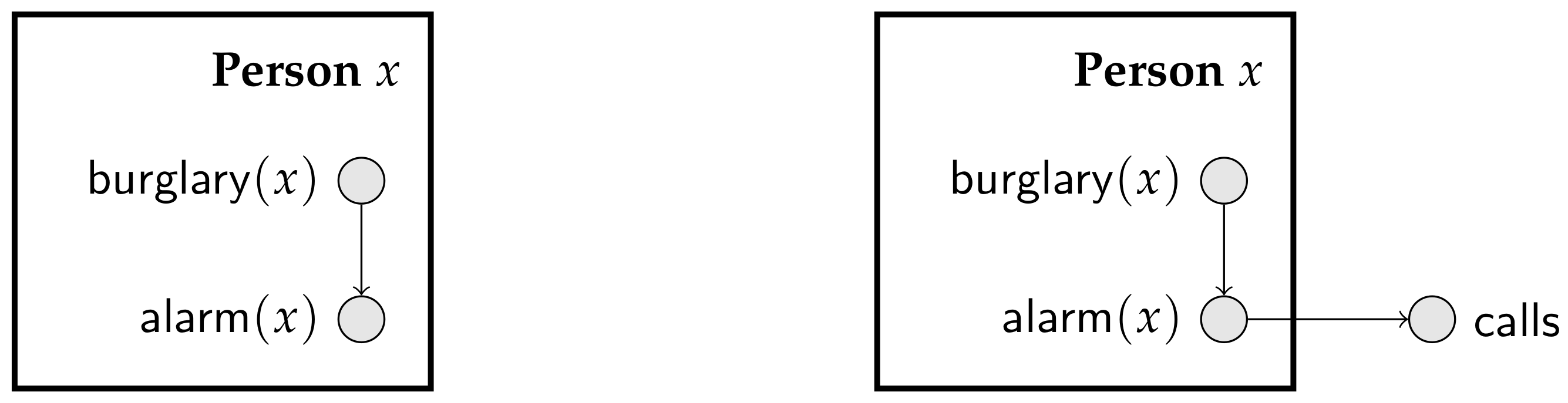
Figure 4.
A Probabilistic Relational Model (PRM) for Scenario 4 in Example 2, using a diagrammatic scheme suggested by Getoor et al. [19]. A textual description of this PRM is presented in Section 4.
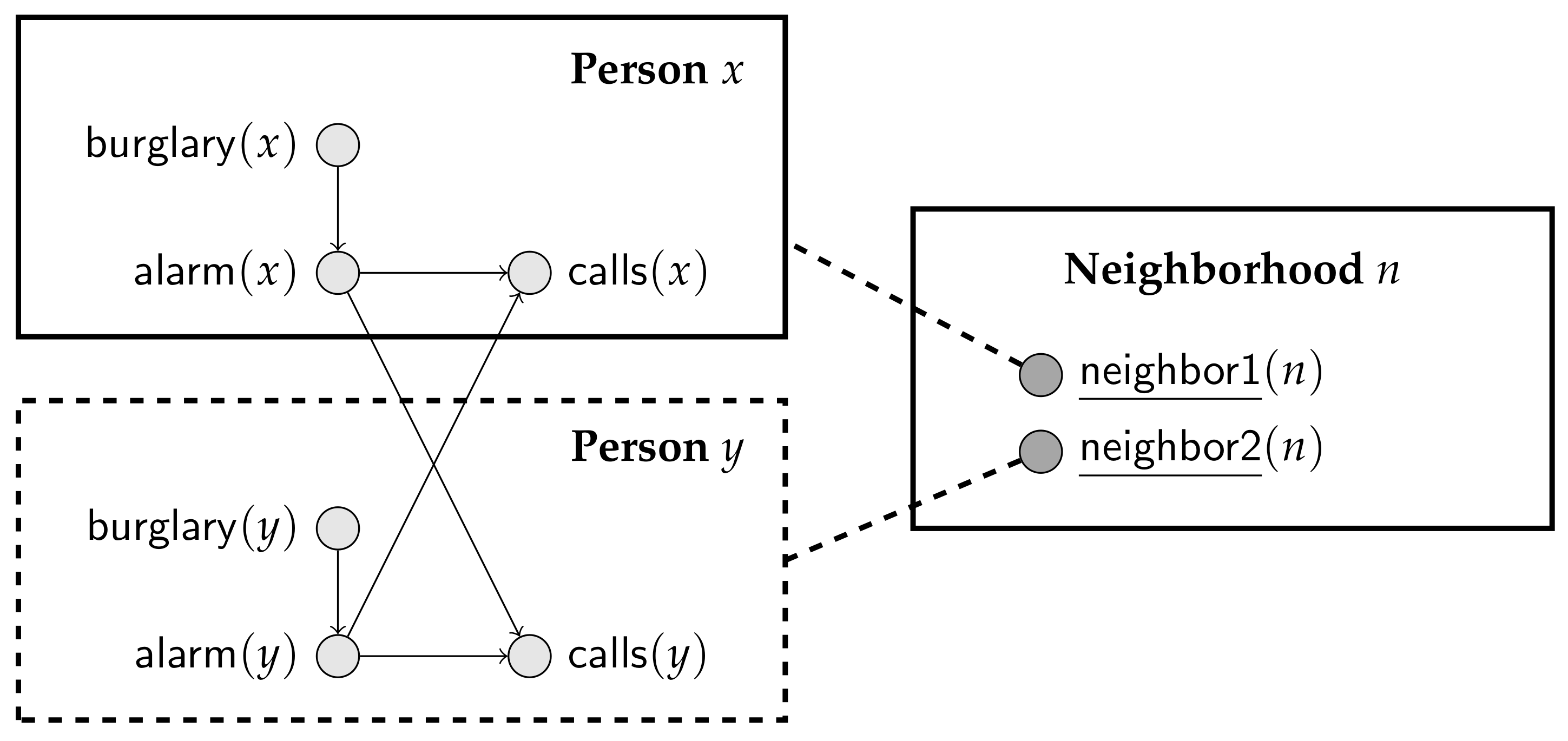
Figure 5.
The PRM for the genetic example, as proposed by Getoor et al. [19].
Figure 5.
The PRM for the genetic example, as proposed by Getoor et al. [19].

© 2018 by the authors. Licensee MDPI, Basel, Switzerland. This article is an open access article distributed under the terms and conditions of the Creative Commons Attribution (CC BY) license (http://creativecommons.org/licenses/by/4.0/).
Share and Cite
MDPI and ACS Style
De Bona, G.; Cozman, F.G. On the Coherence of Probabilistic Relational Formalisms. Entropy 2018, 20, 229. https://doi.org/10.3390/e20040229
AMA Style
De Bona G, Cozman FG. On the Coherence of Probabilistic Relational Formalisms. Entropy. 2018; 20(4):229. https://doi.org/10.3390/e20040229
Chicago/Turabian StyleDe Bona, Glauber, and Fabio G. Cozman. 2018. "On the Coherence of Probabilistic Relational Formalisms" Entropy 20, no. 4: 229. https://doi.org/10.3390/e20040229
Note that from the first issue of 2016, this journal uses article numbers instead of page numbers. See further details here.