Robust Covariance Estimators Based on Information Divergences and Riemannian Manifold


School of Electronic Science, National University of Defence Technology, Changsha 410073, China
*
Authors to whom correspondence should be addressed.
Entropy 2018, 20(4), 219; https://doi.org/10.3390/e20040219
Submission received: 25 February 2018
/
Revised: 12 March 2018
/
Accepted: 12 March 2018
/
Published: 23 March 2018
(This article belongs to the Section Information Theory, Probability and Statistics)
Abstract
:This paper proposes a class of covariance estimators based on information divergences in heterogeneous environments. In particular, the problem of covariance estimation is reformulated on the Riemannian manifold of Hermitian positive-definite (HPD) matrices. The means associated with information divergences are derived and used as the estimators. Without resorting to the complete knowledge of the probability distribution of the sample data, the geometry of the Riemannian manifold of HPD matrices is considered in mean estimators. Moreover, the robustness of mean estimators is analyzed using the influence function. Simulation results indicate the robustness and superiority of an adaptive normalized matched filter with our proposed estimators compared with the existing alternatives.
1. Introduction
Covariance estimation plays an important role in adaptive signal processing, such as multichannel signal processing [1,2], space-time adaptive processing (STAP) [3,4], and radar target detection. Conventional covariance estimation methods, derived from the maximum-likelihood (ML) of the clutter data, are based on the assumption that the clutter remains stationary and homogeneous during the adaptation process. However, in real heterogeneous clutter, the number of the sample data where the clutter is homogeneous is very limited, and the estimation performance is seriously degraded. Therefore, it is necessary and important to improve the performance of estimated covariance in heterogeneous clutter.
A commonly used strategy to ameliorate the performance of estimated covariance is to exploit some a priori information about the clutter environment. For instance, the geographic information is used for covariance estimation, and the performance of target detection with the estimator is significant improved [5]. In [6], the authors employ the Bayesian method to perform the target detection in interference environment, where the unknown covariance matrix is assumed to follow a suitable probability model. In [7,8], a Bayesian framework is used together with the structural information about the estimated covariance. In [9], a condition number upper-bound constraint is imposed on the problem of covariance estimation to achieve a signal-to-noise ratio improvement. Moreover, a symmetrically structured spectral density is constrained on the covariance estimation, and these results show the superiority of the estimator [10]. These mentioned methods rely on the knowledge of statistics characterization of the clutter data. However, the probability distribution of the whole environment is difficult to obtain, and a mismatched distribution results in a remarkable degradation of the estimation performance in heterogeneous clutter.
Many covariance estimation algorithms derived from the geometry of matrix space, not resorting to the statistical characterization of the sample data, are reported in the literature. For instance, the Riemannian mean is used for monitoring the wake turbulence [11,12] and target detection in HF and X-band radar [13]. In [14,15,16], Riemannian mean and median are employed for covariance estimation in STAP, and results have shown that the projection algorithm with Riemannian mean can yield significant performance gains. In [17,18], some geometric barycenter and medians are proposed for radar training data selection in homogeneous environment. In recent times, we have explored information divergence means and medians for target detection in non-Gaussian clutter [19,20,21]. Moreover, in image processing applications, Bhattacharyya mean and median are used for filtering and clustering of diffusion tensor magnetic resonance image [22,23]. In [24], the Log-Euclidean mean, together with the reproducing kernel Hilbert mapping, is used for texture recognition. These geometric approaches have achieved good performances.
In this paper, a class of covariance estimators based on information divergences is proposed in heterogeneous clutter. In particular, six means related to geometric measures are derived on the Riemannian manifold of Hermitian positive-definite (HPD) matrices. These means do not rely on the knowledge of statistics characterization of sample data, and the geometry of the matrix space is considered. Moreover, the robustness of means is analyzed with injected outliers via the influence function. Simulation results are given to validate the superiority of proposed estimators.
The rest of this paper is organized as follows. In Section 2, we reformulate the problem of covariance estimation on the Riemannian manifold. In Section 3, the geometry of Riemannian manifold of HPD matrices is presented, in particular, six distance measures are given on the Riemannian manifold, and means associated with these measures are derived. The robustness of means is analyzed via the influence function in Section 4. Then, we evaluate performances of an adaptive normalized matched filter with geometric means as well as the normalized sample covariance matrix in Section 5. Finally, conclusion is provided in Section 6.
Notation
Here is some notation for the descriptions of this article. A matrix and a vector are noted as uppercase bold and lowercase bold, respectively. The conjugate transpose of matrix is denoted as . is the trace of matrix . is the determinant of matrix . denotes the identity matrix. Finally, denotes the statistical expectation.
2. Problem Reformulated on the Riemannian Manifold
A heterogeneous environment is considered for covariance estimation. For a set of K secondary data , the normalized sample covariance matrix (NSCM) based on the ML of probability distribution of the sample data is estimated as,
where N is the dimension of the vector . are modeled as a compound-Gaussian random vector, and can be expressed as,
where is a nonnegative scalar random variable, and is a N-dimensional circularly symmetric zero-mean vectors with an arbitrary joint statistical distribution and sharing the same covariance matrix,
It is clear from Equation (1) that the NSCM is the arithmetic mean of K auto-covariance matrices of rank one. Since the knowledge of probability distribution of the whole environment is difficult to obtain in heterogeneous clutter, the performance of NSCM is severely degraded. Actually, these K auto-covariance matrices lie in a non-linear Hermitian matrix space, as the sample data is complex. It is well known that HPD matrices form a differentiable Riemannian manifold [25], that is the most studied example of a manifold with non-positive curvature [26]. In order to facilitate the analysis, the matrix is transformed to the positive- definite matrix using the following three ways:
- (1) is obtained by adding an identity matrix , as ;
- (2) A Toeplitz HPD matrix is utilized. As in [13], can be expressed as,where denotes the correlation coefficient of sample data, and is the complex conjugate of . can be computed as,
- (3) The HPD matrix is the solution of the optimization problem as follows [17],
The optimal solution can be given by [17],
where is a unitary matrix of the eigenvectors of with the first eigenvector corresponding to the eigenvalue . The is the condition number.
According to above transformations, we can obtain the HPD matrix. Then, the problem of covariance estimation can be reformulated on the Riemannian manifold. In general, for a set of m scalar numbers , the arithmetic mean is defined as the minimum of sum of squared distances to the given point x,
From Equation (8), we can understand the arithmetic mean from a geometric viewpoint. Similar to Equation (8), for K HPD matrices , the mean related to a measure can be defined as,
where denotes the measure. It is worth pointing out that the arithmetic mean Equation (1) is obtained, when d is the Frobenius norm and is replaced by . The difference between the arithmetic mean and the geometric mean is shown in Figure 1. As illustrated in Figure 1, the geometric median is performed on the Riemannian manifold of HPD matrices with a non-Euclidean metric, whereas the arithmetic mean is considered in the Euclidean space. The difference implies that the different geometric structures are considered in these two estimators.
3. The Geometry of Riemannian Manifold of HPD Matrices
In this Section, the fundamental mathematic knowledge related to this paper is presented. Firstly, the Riemannian manifold of HPD matrices is introduced. Then, six distance measures are presented. Finally, the means related to measures are derived.
3.1. The Riemannian Manifold of HPD Matrices
Let denotes the space of Hermitian matrix. For a Hermitian matrix , if the quadratic form , then, is an HPD matrix, where is the space of n-dimensional complex vector. All HPD matrices consist of a positive-definite Hermitian matrix space ,
forms a Riemannian manifold of dimension with a constant non-positive curvature [26]. For a point on the Riemannian manifold, the infinitesimal arclength between and is given by [27],
where defines a metric on the Riemannian manifold [27]. is the Frobenius norm of a matrix. The inner product and corresponding norm on the tangent space at the point can be defined as [28],
For two points and on the Riemannian manifold, the affine invariant (Riemannian) distance is given by [29],
where is the logarithmic map on the Riemannian manifold of HPD matrices.
3.2. The Geometric Measure on the Riemannian Manifold
In addition to the Riemannian distance, a lot of distance or information divergences can be used as the measurement on the Riemannian manifold. Here, five geometric measures are presented in the following.
(1) Log-Euclidean distance
The Log-Euclidean distance is also a geodesic distance. It is defined on the tangent space at a point on the Riemannian manifold, which is isomorphic and diffeomorphic to the tangent space identified with a Hermitian matrix space. For two points and , the Log-Euclidean distance is given by [30],
(2) Hellinger distance
The Hellinger distance is a special case of the -divergence with . Given two points and , the Hellinger distance is [31],
(3) Kullback-Leibler divergence
It is well known that the Kullback-Leibler (KL) divergence is the most widely used measure on the Riemannian manifold. The KL divergence is also a special case of the -divergence with . In addition, the KL divergence is called the Stein loss or the log-determinant divergence. The KL divergence between two points and can be given by [32],
(4) Bhattacharyya distance
The Bhattacharyya distance is a common used measure, and has been used in medical image segmentation [22]. In particular, the Bhattacharyya distance is a Jensen version of the KL divergence. For two points and , the Bhattacharyya distance can be given by,
(5) Symmetrized Kullback-Leibler divergence
The symmetrized Kullback-Leibler (SKL) divergence is a Jeffreys divergence [33]. It behaves as the square of a distance; however, it is not a distance, as the triangle inequality does not hold. Given two points and , the SKL between them is,
3.3. The Geometric Mean for A Set of HPD Matrices
4. Robustness Analysis of Geometric Means
This section is devoted to analyzing the robustness of geometric means via the influence function. Let be the mean, associated with a measure, of m HPD matrices . is the mean by adding a set of n outliers with a weight to . Then, we can define , denotes the influence function. In the following, seven propositions are presented.
Proposition 1.
The influence function of arithmetic mean related to the Frobenius norm, of m HPD matrices and n outliers is given by,
Proof of Proposition 1.
Let be the objection function,
The derivative of objection function is,
Note that is the mean of m matrices and n outliers, and is the mean of m matrices, then, we have,
and
Substitute into Equation (22), and we have
☐
Proposition 2.
The influence function of Riemannian mean related to the Riemannian distance, of m HPD matrices and n outliers is given by,
Proof of Proposition 2.
Let be the objection function,
As is the mean of m matrices and n outliers, and is the mean of m matrices, then, we have,
and
Using the Taylor expansion on , and we have
Ignore the terms contain for the constant , and we can obtain,
☐
Proposition 3.
The influence function of Log-Euclidean mean related to the Log-Euclidean distance, of m HPD matrices and n outliers is given by,
Proof of Proposition 3.
Let be the objection function,
Note that is the mean of m matrices and n outliers, and is the mean of m matrices, then, we have,
and
Using the Taylor expansion on , and we have
Proposition 4.
The influence function of Hellinger mean related to the Hellinger distance, of m HPD matrices and n outliers is given by,
Proof of Proposition 4.
Let be the objection function,
Note that is the mean of m matrices and n outliers, and is the mean of m matrices, then, we have,
and
Using the Taylor expansion on , and we have
Proposition 5.
The influence function of KL mean related to the KL divergence, of m HPD matrices and n outliers is given by,
Proof of Proposition 5.
Let be the objection function,
As is the mean of m matrices and n outliers, and is the mean of m matrices, then, we have,
and
Using the Taylor expansion on , and we have,
Proposition 6.
The influence function of Bhattacharyya mean related to the Bhattacharyya divergence, of m HPD matrices and n outliers is given by,
Proof of Proposition 6.
Let be the objection function,
Note that is the mean of m matrices and n outliers, and is the mean of m matrices, then, we have,
and
Using the Taylor expansion on , and we have,
Proposition 7.
The influence function of SKL mean related to the SKL divergence, of m HPD matrices and n outliers is given by,
5. Numerical Simulations
In order to gain a better understanding of the superiority of proposed estimators, simulation results of the performance of an ANMF with the proposed estimator in heterogeneous clutter are presented. As there is not an analytical expression for the detection threshold, the standard Monte Carlo technique [34] is utilized. A similar approach was recently used to solve several problems from different areas, such as physics [35], decision theory [36], engineering [37], computational geometry [38], finance [39], etc. The rule of adaptive normalized matched filter (ANMF) is given as [40],
where is the clutter covariance estimation. is the sample data in the cell under test. denotes the threshold, which is derived by Monte Carlo method in order to maintain the false alarm constant. is the target steering vector, and is given by,
where is the normalized Doppler frequency. According to Equation (2), the terms are compound-Gaussian random vectors, and sharing the same covariance matrix ,
where is accounting for the thermal noise. is related to the clutter, modeled as,
where is the one-lag correlation coefficient. is the clutter-to-noise power ratio. is the clutter normalized Doppler frequency.
In addition, and are positive and real independent and identical distributed random variables, and are assumed to follow the inverse gamma distribution,
where and denote the shape and scale parameters, respectively. is the gamma function. In the simulation, we set , , and dB. The parameters , and .
In the following, we analyze the performance of an ANMF with the proposed estimators, in terms of detection probability (), also in comparison with the optimum detector, which assumes the perfect knowledge of the disturbance covariance matrix, NMF. In particular, the positive-definite matrix obtained using (1), (2), and (3) is noted as the SPDF, THPD, and SPD matrix, respectively. Simulation results are shown in Figure 2 with , , it is clear that the proposed estimators have different performances, and all the proposed estimators have better performances than the NSCM estimator when and . In particular, our proposed estimators have different performance when different positive-definite matrix is utilized. For the SPDF positive-definite matrix, the Bhat estimator, the Hel estimator, and the KL estimator have comparable performances, and outperform others. The SKL estimator has the worst performance, while the KL estimator has the best performance. However, this relationship is different on the condition of the THPD positive-definite matrix. Particularly, performances of the KL estimator and the SKL estimator are poor. Performances of the other proposed estimators are close to the optimum. For the SPD positive-definite matrix, relationships of proposed estimators are similar to the case of SPDF positive-definite matrix. The KL estimator has the best performance, while the performance of SKL estimator is the worst. In addition, the performance of Hel estimator is poor. These results imply that performances of proposed estimators are related to the used positive-definite matrix.
In order to show the influence function of robustness of proposed estimators, 17 positive-definite matrices with an injected outlier are considered. The value of influence function is computed as Propositions 1–7, and 100 times simulations are repeated. A total of 100 simulation results and the average of values of influence function are shown in Figure 3. From Figure 3 we can know that our proposed estimators are more robust than the NSCM estimator. In particular, the robustness of SKL estimator is poor, while the KL estimator has the best robustness when the SPDF or THPD positive-definite matrix is utilized. For the SPD positive-definite matrix, all proposed estimators have comparable robustness. It can be concluded that the robustness of proposed estimators is related to the used positive-definite matrix. It is worth pointing out that the three HPD matrices, namely the SPDF, THPD, and SPD matrix, have different structures. Both the SPDF and the SPD matrices have a largest eigenvalue and equal eigenvalues. Their differences lie in the multiple between the maximum eigenvalue and the minimum eigenvalue. In particular, this multiple of the SPD matrix is the constant number , while the SPDF matrix has a varied multiple. For the THPD matrix, all eigenvalues are different. Riemannian manifolds composed of different positive-definite matrices have different geometric structures. Thus, the estimators associated with different metrics on Riemannian manifold may have different behaviors.
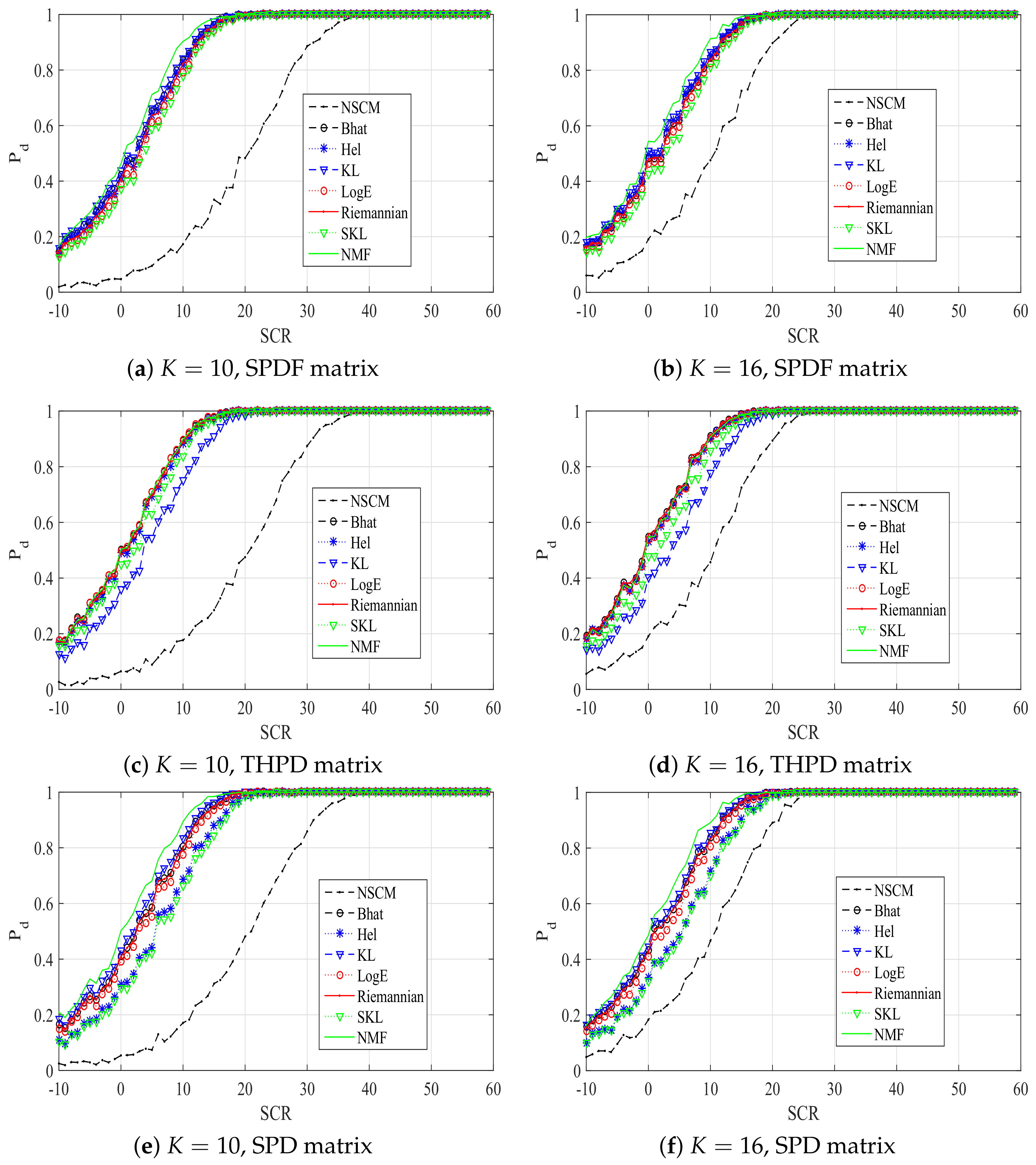
Figure 4 plots the of the ANMF with our proposed estimators, the NSCM estimator, and the NMF detector in a contaminated clutter. An outlier is injected in one reference cell, the number of reference cell K is set to 10 and 16, respectively. The dimension of the sample data is 8. It can be noted from Figure 4 that performances of our proposed estimators have not been significantly reduced, while there is a degradation in the performance of the NSCM estimator. Relationships of performances are similar to curves of Figure 2. These results prove the advantage of our proposed estimators sufficiently.
6. Conclusions
In this paper, a class of covariance estimators based on information divergences is proposed in heterogeneous clutter. Particularly, the problem of disturbance covariance estimation is reformulated as obtaining the geometric mean on the Riemannian manifold. Six mean estimators related to information measures are derived. Moreover, the robustness of proposed estimators are analyzed via the influence function, and the analytic expression of influence function is deduced. At the analysis stage, the performance advantage and robustness of our proposed estimators are verified by means of simulation results in heterogeneous environment.
Acknowledgments
This work was supported by the National Natural Science Foundation of China under grant No. 61302149. The authors are grateful for the valuable comments made by the reviewers, which have assisted us with a better understanding of the underlying issues and therefore a significant improvement in the quality of the paper.
Author Contributions
Xiaoqiang Hua put forward the original ideas and performed the research. Yongqiang Cheng conceived and designed the simulations. Hongqiang Wang and Yuliang Qin reviewed the paper and provided useful comments. All authors have read and approved the final manuscript.
Conflicts of Interest
The authors declare no conflict of interest.
References
- Visuri, S.; Oja, H.; Koivunen, V. Multichannel signal processing using spatial rank covariance matrices. In Proceedings of the IEEE Eurasip Workshop on Nonlinear Signal and Image Processing, Antalya, Turkey, 20–23 June 1999; pp. 75–79. [Google Scholar]
- Williams, D.B.; Johnson, D.H. Robust estimation of structured covariance matrices. IEEE Trans. Signal Process. 1993, 41, 2891–2906. [Google Scholar] [CrossRef]
- Barton, T.; Smith, S. Structured Covariance Estimation for Space-Time Adaptive Processing. In Proceedings of the IEEE International Conference on Acoustics, Speech, and Signal Processing, Munich, Germany, 21–24 April 1997; pp. 3493–3496. [Google Scholar]
- Semeniaka, A.V.; Lekhovitskiy, D.I.; Rachkov, D.S. Comparative analysis of Toeplitz covariance matrix estimation methods for space-time adaptive signal processing. In Proceedings of the IEEE CIE International Conference on Radar, Chengdu, China, 24–27 October 2011; pp. 696–699. [Google Scholar]
- Maio, A.D.; Farina, A.; Foglia, G. Design and experimental validation of knowledge-based constant false alarm rate detectors. IET Radar Sonar Navig. 2007, 1, 308–316. [Google Scholar] [CrossRef]
- Maio, A.D.; Farina, A.; Foglia, G. Knowledge-Aided Bayesian Radar Detectors Their Application to Live Data. IEEE Trans. Aerosp. Electron. Syst. 2010, 46, 170–183. [Google Scholar] [CrossRef]
- Wang, P.; Li, H.; Himed, B. Knowledge-Aided Parametric Tests for Multichannel Adaptive Signal Detection. IEEE Trans. Signal Process. 2011, 59, 5970–5982. [Google Scholar] [CrossRef]
- Li, H.; Michels, J.H. Parametric adaptive signal detection for hyperspectral imaging. IEEE Trans. Signal Process. 2006, 54, 2704–2715. [Google Scholar]
- Aubry, A.; Maio, A.D.; Pallotta, L.; Farina, A. Maximum Likelihood Estimation of a Structured Covariance Matrix with a Condition Number Constraint. IEEE Trans. Signal Process. 2012, 60, 3004–3021. [Google Scholar] [CrossRef]
- Maio, A.D.; Orlando, D.; Foglia, G.; Foglia, G. Adaptive Detection of Point-Like Targets in Spectrally Symmetric Interference. IEEE Trans. Signal Process. 2016, 64, 3207–3220. [Google Scholar] [CrossRef]
- Liu, Z.; Barbaresco, F. Doppler Information Geometry for Wake Turbulence Monitoring; Springer: Berlin/Heidelberg, Germany, 2013. [Google Scholar]
- Barbaresco, F.; Meier, U. Radar monitoring of a wake vortex: Electromagnetic reflection of wake turbulence in clear air. C. R. Phys. 2010, 11, 54–67. [Google Scholar] [CrossRef]
- Lapuyade-Lahorgue, J.; Barbaresco, F. Radar detection using Siegel distance between autoregressive processes, application to HF and X-band radar. In Proceedings of the IEEE Radar Conference, Rome, Italy, 26–30 May 2008; pp. 1–6. [Google Scholar]
- Balaji, B.; Barbaresco, F. Application of Riemannian mean of covariance matrices to space-time adaptive processing. In Proceedings of the IEEE Radar Conference, Amsterdam, The Netherlands, 31 October–2 November 2012; pp. 50–53. [Google Scholar]
- Balaji, B. Riemannian mean and space-time adaptive processing using projection and inversion algorithms. Proc. SPIE 2013, 8714, 813–831. [Google Scholar]
- Barbaresco, F. Robust statistical Radar Processing in Frechet metric space: OS-HDR-CFAR and OS-STAP Processing in Siegel homogeneous bounded domains. In Proceedings of the International Radar Symposium (IRS), Leipzig, Germany, 7–9 September 2011; pp. 639–644. [Google Scholar]
- Aubry, A.; Maio, A.D.; Pallotta, L.; Farina, A. Covariance matrix estimation via geometric barycenters and its application to radar training data selection. IET Radar Sonar Navig. 2013, 7, 600–614. [Google Scholar] [CrossRef]
- Aubry, A.; Maio, A.D.; Pallotta, L.; Farina, A. Median matrices and their application to radar training data selection. IET Radar Sonar Navig. 2013, 8, 265–274. [Google Scholar] [CrossRef]
- Hua, X.; Cheng, Y.; Wang, H.; Qin, Y.; Li, Y. Geometric means and medians with applications to target detection. IET Signal Process. 2017, 11, 711–720. [Google Scholar] [CrossRef]
- Hua, X.; Cheng, Y.; Wang, H.; Qin, Y.; Li, Y.; Zhang, W. Matrix CFAR detectors based on symmetrized Kullback Leibler and total Kullback Leibler divergences. Digit. Signal Process. 2017, 69, 106–116. [Google Scholar] [CrossRef]
- Hua, X.; Cheng, Y.; Li, Y.; Shi, Y.; Wang, H.; Qin, Y. Target Detection in Sea Clutter via Weighted Averaging Filter on the Riemannian Manifold. Aerosp. Sci. Technol. 2017, 70. [Google Scholar] [CrossRef]
- Charfi, M.; Chebbi, Z.; Moakher, M.; Vemuri, B.C. Using the Bhattacharyya Mean for the Filtering and Clustering of Positive-Definite Matrices. In Proceedings of the Geometric Science of Information: First International Conference, GSI 2013, Paris, France, 28–30 August 2013; pp. 551–558. [Google Scholar]
- Charfi, M.; Chebbi, Z.; Moakher, M.; Vemuri, B.C. Bhattacharyya median of symmetric positive-definite matrices and application to the denoising of diffusion-tensor fields. In Proceedings of the IEEE International Symposium on Biomedical Imaging, San Francisco, CA, USA, 7–11 April 2013; pp. 1227–1230. [Google Scholar]
- Jayasumana, S.; Hartley, R.; Salzmann, M.; Li, H.; Harandi, M. Kernel Methods on the Riemannian Manifold of Symmetric Positive Definite Matrices. Comput. Vis. Pattern Recog. 2013, 73–80. [Google Scholar]
- Hiai, F.; Petz, D. Riemannian metrics on positive definite matrices related to means. Linear Algebra Appl. 2008, 430, 3105–3130. [Google Scholar] [CrossRef]
- Sra, S. Positive definite matrices and the S divergence. Proc. Am. Math. Soc. 2011, 144, 1–25. [Google Scholar] [CrossRef]
- Moakher, M. On the Averaging of Symmetric Positive Definite Tensors. J. Elast. 2006, 82, 273–296. [Google Scholar] [CrossRef]
- Lang, S. Fundamentals of differential geometry. In Graduate Texts in Mathematics; Springer: New York, NY, USA, 1946; pp. 1757–1764. [Google Scholar]
- Moakher, M. A Differential Geometric Approach to the Geometric Mean of Symmetric Positive-Definite Matrices. Siam J. Matrix Anal. Appl. 2008, 26, 735–747. [Google Scholar] [CrossRef]
- Arsigny, V.; Fillard, P.; Pennec, X.; Ayache, N. Log-Euclidean metrics for fast and simple calculus on diffusion tensors. Magn. Reson. Med. 2006, 56, 411–421. [Google Scholar] [CrossRef] [PubMed]
- Lindsay, B.G. Efficiency Versus Robustness: The Case for Minimum Hellinger Distance and Related Methods. Ann. Stat. 1994, 22, 1081–1114. [Google Scholar] [CrossRef]
- Csiszar, I. Why Least Squares and Maximum Entropy? An Axiomatic Approach to Inference for Linear Inverse Problems. Ann. Stat. 1991, 19, 2032–2066. [Google Scholar] [CrossRef]
- Menendez, M.L.; Pardo, J.A.; Pardo, L.; Pardo, M.C. The Jensen-Shannon divergence. J. Frankl. Inst. 1997, 334, 307–318. [Google Scholar] [CrossRef]
- Fishman, G.S. Monte Carlo. Concepts, algorithms, and applications. Technometrics 1996, 39, 338. [Google Scholar]
- Klein, S.R.; Nystrand, J.; Seger, J.; Gorbunov, Y.; Butterworth, J. STARlight: A Monte Carlo simulation program for ultra peripheral collisions of relativistic ions. Comput. Phys. Commun. 2016, 212, 258–268. [Google Scholar] [CrossRef]
- Pask, F.; Lake, P.; Yang, A.; Tokos, H.; Sadhukhan, J. Sustainability indicators for industrial ovens and assessment using Fuzzy set theory and Monte Carlo simulation. J. Clean. Prod. 2016, 140, 1217–1225. [Google Scholar] [CrossRef]
- Ma, Y.; Chen, X.; Biegler, L.T. Monte Carlo simulation-based optimization for copolymerization processes with embedded chemical composition distribution. Comput. Chem. Eng. 2018, 109, 261–275. [Google Scholar] [CrossRef]
- Vilcu, A.D.; Vilcu, G.E. An algorithm to estimate the vertices of a tetrahedron from uniform random points inside. Ann. Mat. Pura Appl. 2016, 4, 1–14. [Google Scholar] [CrossRef]
- Bormetti, G.; Callegaro, G.; Livieri, G.; Pallavicini, A. A backward Monte Carlo approach to exotic option pricing. Eur. J. Appl. Math. 2018, 29, 146–187. [Google Scholar] [CrossRef]
- Conte, E.; Lops, M.; Ricci, G. Adaptive detection schemes in compound-Gaussian clutter. IEEE Trans. Aerosp. Electron. Syst. 1998, 34, 1058–1069. [Google Scholar] [CrossRef]
Figure 1.
The geometric mean and the arithmetic mean.
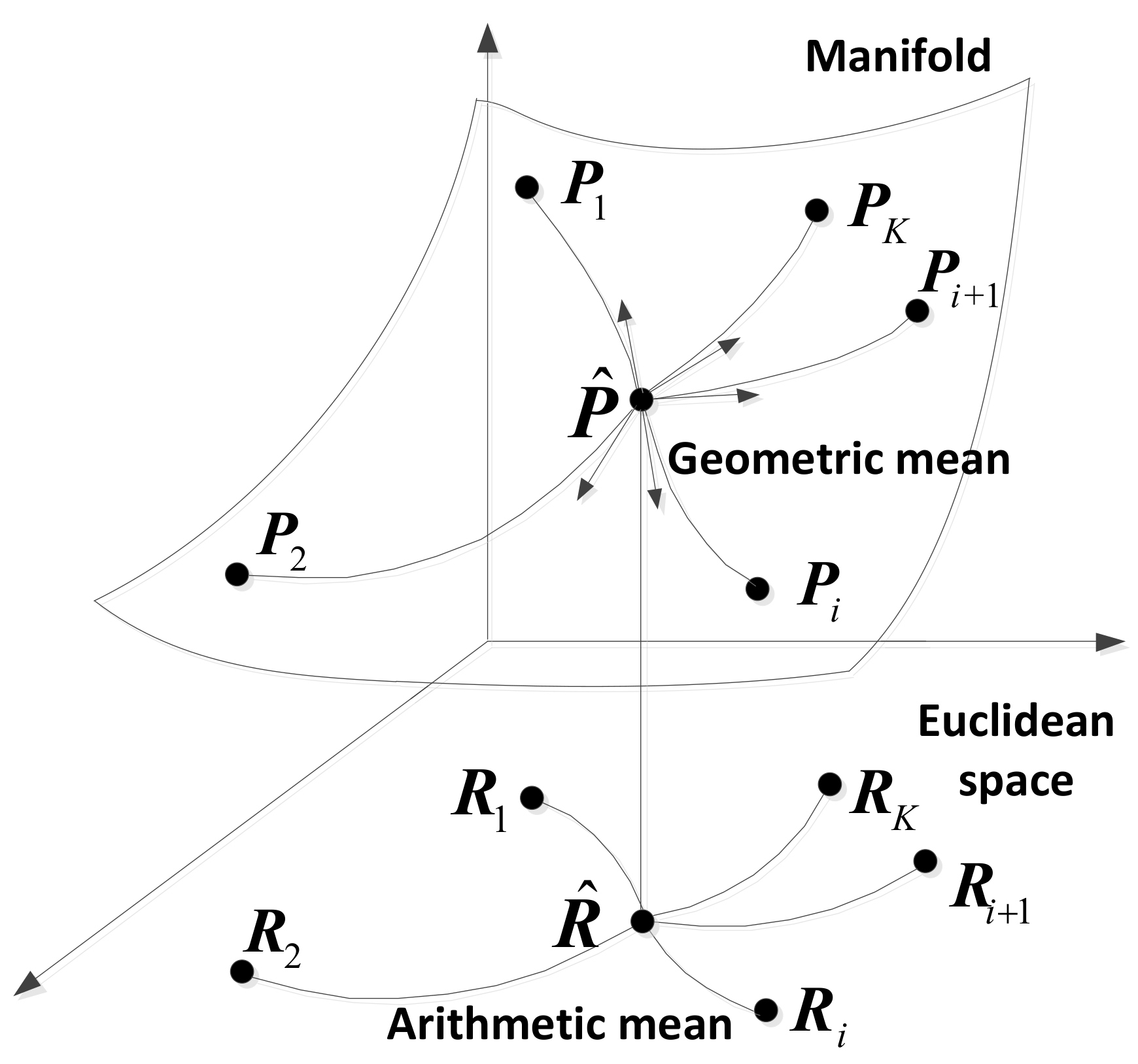
Figure 2.
versus SCR plots of ANMFs with proposed estimators, the NSCM estimator, and NMF.

Figure 3.
The error value of proposed estimators and their corresponding mean vlaue.
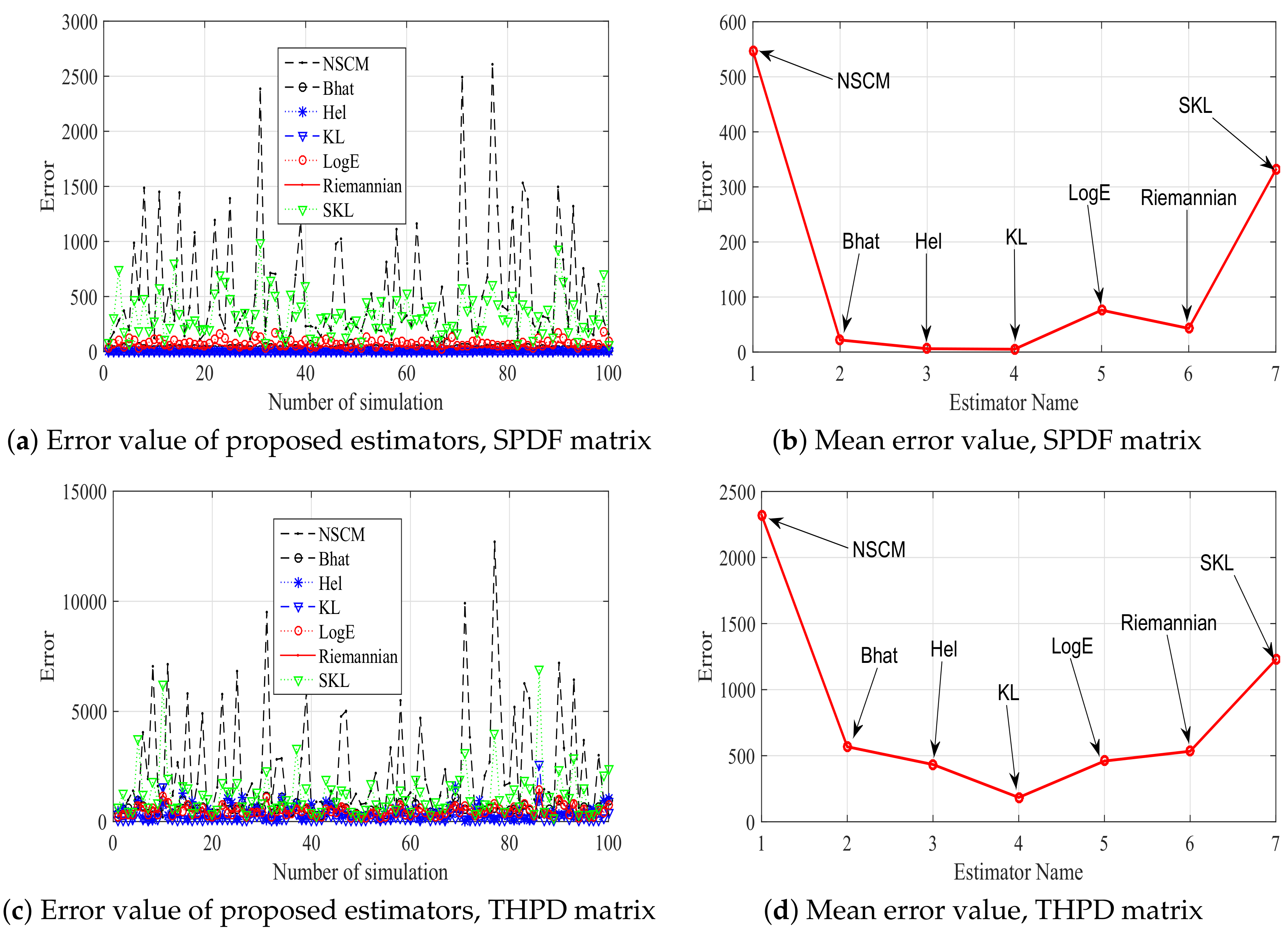
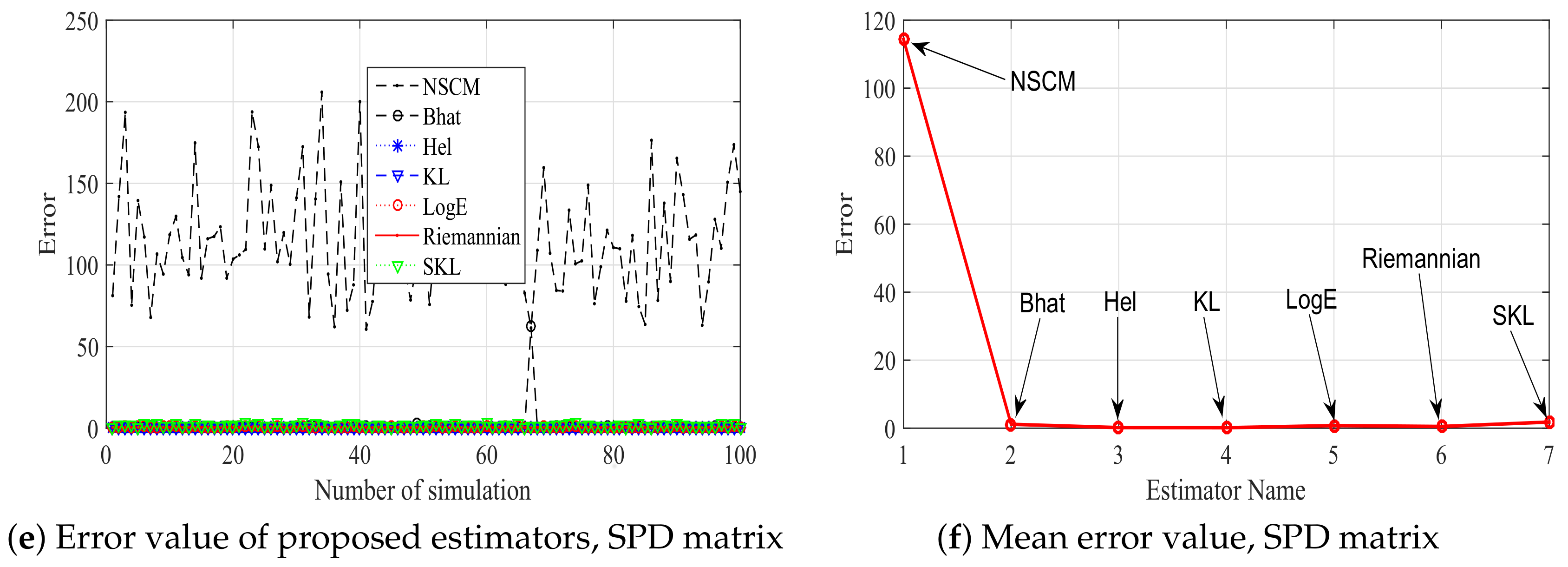
Figure 4.
versus SCR plots of ANMFs with proposed estimators, the NSCM estimator, and NMF in a contaminated environment.
Figure 4.
versus SCR plots of ANMFs with proposed estimators, the NSCM estimator, and NMF in a contaminated environment.

Table 1.
Geometric means related to different measures.
| Geometric Measure | Mean |
|---|---|
| Riemannian | |
| Log-Euclidean | |
| Hellinger | |
| KL | |
| Bhattacharyya | |
| SKL |
Where t is the number of iteration, and is is the step size of iteration.
© 2018 by the authors. Licensee MDPI, Basel, Switzerland. This article is an open access article distributed under the terms and conditions of the Creative Commons Attribution (CC BY) license (http://creativecommons.org/licenses/by/4.0/).
Share and Cite
MDPI and ACS Style
Hua, X.; Cheng, Y.; Wang, H.; Qin, Y. Robust Covariance Estimators Based on Information Divergences and Riemannian Manifold. Entropy 2018, 20, 219. https://doi.org/10.3390/e20040219
AMA Style
Hua X, Cheng Y, Wang H, Qin Y. Robust Covariance Estimators Based on Information Divergences and Riemannian Manifold. Entropy. 2018; 20(4):219. https://doi.org/10.3390/e20040219
Chicago/Turabian StyleHua, Xiaoqiang, Yongqiang Cheng, Hongqiang Wang, and Yuliang Qin. 2018. "Robust Covariance Estimators Based on Information Divergences and Riemannian Manifold" Entropy 20, no. 4: 219. https://doi.org/10.3390/e20040219
Note that from the first issue of 2016, this journal uses article numbers instead of page numbers. See further details here.