Optomechanical Analogy for Toy Cosmology with Quantized Scale Factor


1
Joint Center for Quantum Information and Computer Science, College Park, MD 20742, USA
2
Joint Quantum Institute/NIST, College Park, MD 20742, USA
3
Research Center for Advanced Science and Technology, Tokyo 153-0041, Japan
*
Author to whom correspondence should be addressed.
Entropy 2017, 19(9), 485; https://doi.org/10.3390/e19090485
Submission received: 30 June 2017
/
Revised: 23 August 2017
/
Accepted: 8 September 2017
/
Published: 12 September 2017
(This article belongs to the Collection Quantum Information)
Abstract
:The simplest cosmology—the Friedmann–Robertson–Walker–Lemaître (FRW) model— describes a spatially homogeneous and isotropic universe where the scale factor is the only dynamical parameter. Here we consider how quantized electromagnetic fields become entangled with the scale factor in a toy version of the FRW model. A system consisting of a photon, source, and detector is described in such a universe, and we find that the detection of a redshifted photon by the detector system constrains possible scale factor superpositions. Thus, measuring the redshift of the photon is equivalent to a weak measurement of the underlying cosmology. We also consider a potential optomechanical analogy system that would enable experimental exploration of these concepts. The analogy focuses on the effects of photon redshift measurement as a quantum back-action on metric variables, where the position of a movable mirror plays the role of the scale factor. By working in the rotating frame, an effective Hubble equation can be simulated with a simple free moving mirror.
1. Introduction
Quantum mechanics provides several key mechanisms for proposed explanations of cosmological structure [1]. For example, one of the major observational discoveries in cosmology is that the universe is expanding [2,3]. Many puzzles about this expansion, particularly at early time, seem to hinge upon the quantum behavior of the universe’s structure, that is, its metric [4]. A key question in these puzzles is the role decoherence may play in freezing-in quantum fluctuations [5]. In establishing a model for the universe, one would expect macroscopic objects/events to behave classically [6]. Equivalently, one would expect macroscopic objects to be highly entangled such that the state of an object can be easily restricted by making any related measurement. Thus, any quantum treatment of cosmological variables should result in states highly entangled with that variable.
Some simple models consider various toy cosmologies in which parameters of the metric are treated as quantum variables. For example, reference [7] assumes that the universe’s metric is described by a position wavefunction and considers the resulting implications. Another approach is to describe the cosmology using quantum Brownian motion in a parametric bath as in [8,9]. Here we consider a toy cosmology based upon the Friedmann–Robertson–Walker–Lemaître (FRW) model, where the scale factor is quantized, and a wavefunction describing the state of the metric is defined. This wavefunction is often explored in the context of its dynamics as constrained by the Wheeler–DeWitt equation [10,11,12,13,14]. Recently, there has been some suggestion that weak measurement of metric variables might act analogously to dark energy, again in this quantized FRW setting [15].
In this paper, the properties of a simple but quantum metric are explored to help us illustrate the role weak measurements—here mediated by photon emission and absorption—play in stabilizing the metric towards a “classical” state. Thus, all of the underlying factors driving cosmological dynamics (e.g., a perfect fluid [10], imperfect fluid [11], Chaplygin gas [12,13], or field [14]) are ignored, and we do not assume any constraints on dynamics (e.g., the Wheeler–DeWitt equation). Instead, the dynamics of the metric are treated in a general manner as some (specified) unitary evolution, without reference to the source of this cosmological evolution. As such, our approach is, on the one hand, general, but on the other hand, does not provide any answers to questions regarding the meaning of time and related challenges implicit in quantum cosmology. Working in conformal time, we show how photon emission and later absorption leads to a strong entanglement between sources, detectors, and the metric variables. This provides a tool for examining the intuitive result that redshifted photons convey information about the universe’s past and effectively decohere potential superpositions of metric variables.
Direct cosmological experiments are highly limited due to the space and time scales associated with the dynamics. Thus, various analogies are experimentally implemented to explore cosmological effects. For example, superfluid helium models are used to describe freezing-in quantum fluctuations [16,17]. In addition, experiments with Bose–Einstein condensates (BEC) have demonstrated an analogy to Hawking radiation found with black holes [18]. Other analogies consider emulating the space-time, such as with BEC [19], graphene impurities [20], and in an optical lattice [21]. Recently, there was a proposal to emulate an FRW cosmology with circuit-QED using SQUIDS [22]. Using the toy FRW model detailed in this paper, we describe an optomechanical system which possesses analogous properties to an expanding universe. The motion of a mirror in an optical cavity induces a redshift in cavity photons. This process leads to entanglement between an effective scale factor and the sources and detectors that emulates cosmological redshift. Thus we can envision testing quantum cosmology concepts in this toy model setting.
2. The Toy FRW Cosmology
Consider the classical Friedmann-Robertson-Walker (FRW) metric, defined by the line element
where a is the scale factor and is the curvature. Proper time and distance for this metric are described in Figure 1a for an exponentially expanding universe. Naturally, the dynamics of this metric will affect the motion and other dynamics of objects within the metric.
Photons, for example, are known to be affected by the cosmological scale factor. In particular, the expanding universe results in a cosmological redshift from distant objects [2,3]. Classically, if a photon is emitted at frequency at a scale factor of and is later observed at a scale factor of , its observed frequency will be . This frequency shift can be described in the frame of quantum mechanics as entanglement between the universe’s metric and the photon. That is, the dynamics of the photon become “tied’’ to the dynamics of the metric via entanglement. The entanglement between photons and the metric implies that measuring (the redshift of) a photon will restrict the metric’s wavefunction. In a setting with many photons being emitted and detected, as in our actual universe, one would immediately anticipate that observation of redshifted photons tightly constrains the allowed metric, which would dephase superpositions of the metric that are inconsistent with the observed behavior. In that sense, this rapid decoherence of metric superpositions corresponds to a particularly ‘classical’ universe metric. We note that the actual scale factor is not directly observed; rather, it is the proportional change of the scale factor over time that is measured. The manner in which information from the metric is encoded in the photon will be explored.
The FRW metric (Equation (1)) is a simple and highly-symmetric choice, since it is homogeneous and isotropic in spatial slices (i.e., at constant time). Moreover, a single scale factor, , describes the dynamics of the metric. Now, a reparametrization can be applied to the metric to make quantization of the electromagnetic field trivial. Specifically, we move to conformal time, described by the line element:
where describes the conformal time. This coordinate transformation is described in Figure 1b.
Consider the frequency of a photon in an FRW universe. Denote the phase of the photon with . Then, the coordinate frequency is . If , then the coordinate frequency is given by
where is a nominal frequency (taken at some ). Moving to conformal time, the conformal frequency
is then constant in time. This invariance follows from Maxwell’s equations being conformal [23]. Thus, when our only degrees of freedom are photons and the scale factor, it is natural to build the cosmology in conformal time, leading to a simple picture for Hilbert space.
The goal now is to describe a universe in which the scale factor is treated as a quantum variable. After promoting a to an operator , with a corresponding Hilbert space of allowed states, we can define a metric wavefunction in terms of the scale factor eigenbasis
where is the metric wavefunction and is an eigenvector of , satisfying
We would also like to define a logarithmic scale factor, , according to
Observer that this relation is a homeomorphism because the scale factor is always positive; the logarithmic scale factor can be any real number. The logarithmic scale factor has the advantage of possessing translational symmetry in which adding a term corresponds to scaling.
A universe with only a metric and photon degrees of freedom is an extremely poor representation of our own cosmology. Thus, we add matter, but make a simplifying assumption: we assume the matter adiabatically follows the scale factor. We only break this basic story for the photons, which we will allow to be excited away from this nominal matter-universe state. In a fundamental sense, this is looking at only the very lowest energy excitations: photons and gravity. We will denote this matter-simplified toy cosmology “tFRW”.
Consider a simple quantum system consisting of a photon source, detector, vacuum (containing photon modes), and metric. Denote the initial state corresponding to each of these components as
where and refer to the ground and excited states of the source and detector, respectively. Unlike typical treatment of the photon mode, the photon’s conformal frequency is recorded instead of its coordinate frequency. The system will undergo the following process: a photon is emitted from the source, traverses the universe for some time, and then is absorbed/measured by the detector.
Photon emission must then be described in terms of conformal frequency. In coordinate time, the photon frequency is given by the wavepacket, . The emitted wavepacket (in coordinate frequency) is invariant of the scale factor [24,25]. This is equivalent to saying that the local behavior of atoms is independent of the present cosmology. Moving into conformal frequency, , the photon’s conformal frequency wavepacket generator (normalized) becomes
where generates a single conformal frequency mode. Similarly, the photon packet annihilator is
which annihilates the (coordinate frequency) wavepacket given by . Observe that physicality demands the scale factor be strictly positive; a negative scale factor is non-physical, and a zero scale factor corresponds to a singularity (e.g., the Big Bang). In this construction, the sources/detectors will be time-dependent (via coupling to the time-varying metric wavefunction) while the photon mode is time-independent. The wavepacket creation/annihilation operators entangle the photon frequency with the scale factor; the magnitude of a given photon mode is dependent on the state of the metric wavefunction.
A few more operators are needed to fully describe the system. First, the creation operator will have a factor to reflect the source moving to its ground state with the emission of a photon. Similarly, the annihilation operator will have a factor to reflect the absorption of the photon. After detection, the system is projected into the detected state with . Events in which no photon is detected are thrown out as inaccessible; they are inaccessible in the sense that one does not gain any information on the scale factor when no measurement occurs. Thus, the act of measuring is equivalent to post-selecting the universe’s metric in which the measured event occurred. Finally, the metric evolves according to the general (unitary) operator
for some evolution function given in the eigenbasis. The behavior of B is determined by the cosmological equations of state, which in turn could be a complicated system determined by adiabatically following matter-energy state . Here we will neglect the specific role the emitters and detectors play in this equation of state, appropriate for the FRW assumptions.
The system’s evolution is described by
The final state of the metric wavefunction is then
The function
describes how the source/detector wavepackets affect the final state of the universe’s metric. Equation (14) can also be expressed as a function of —this is clear when applying the change-of-variables . This property is expected because photon measurement yields information about the proportion between initial and final scale factors. Observe that Equation (13) demands a proportionality constant. This is to account for the non-zero probability that the photon is not detected. The not-detected state is either removed when applying or throwing out the event altogether as inaccessible via post-selection.
2.1. Simple Examples
Consider a simple evolution in which all scale factors scale by a constant, s. Thus,
where additional corrections necessary to maintain probability (that make B unitary) are neglected for simplicity. Solving for Equation (13):
As one would expect, if is centered around , then is centered around . Moreover, the coefficient is maximized for . That is, if f is centered around , then g is centered around . This is the case when the absorption wavefunction perfectly aligns with the shifted packet so equality now holds in Equation (16).
Now, consider a simple case for the photon wavefunctions. According to Weisskopf–Wigner theory on spontaneous emission, the photon wavefunctions should be Lorentzian [26]:
and
Solving for Equation (14) (integrating over positive and negative frequencies for simplicity) yields
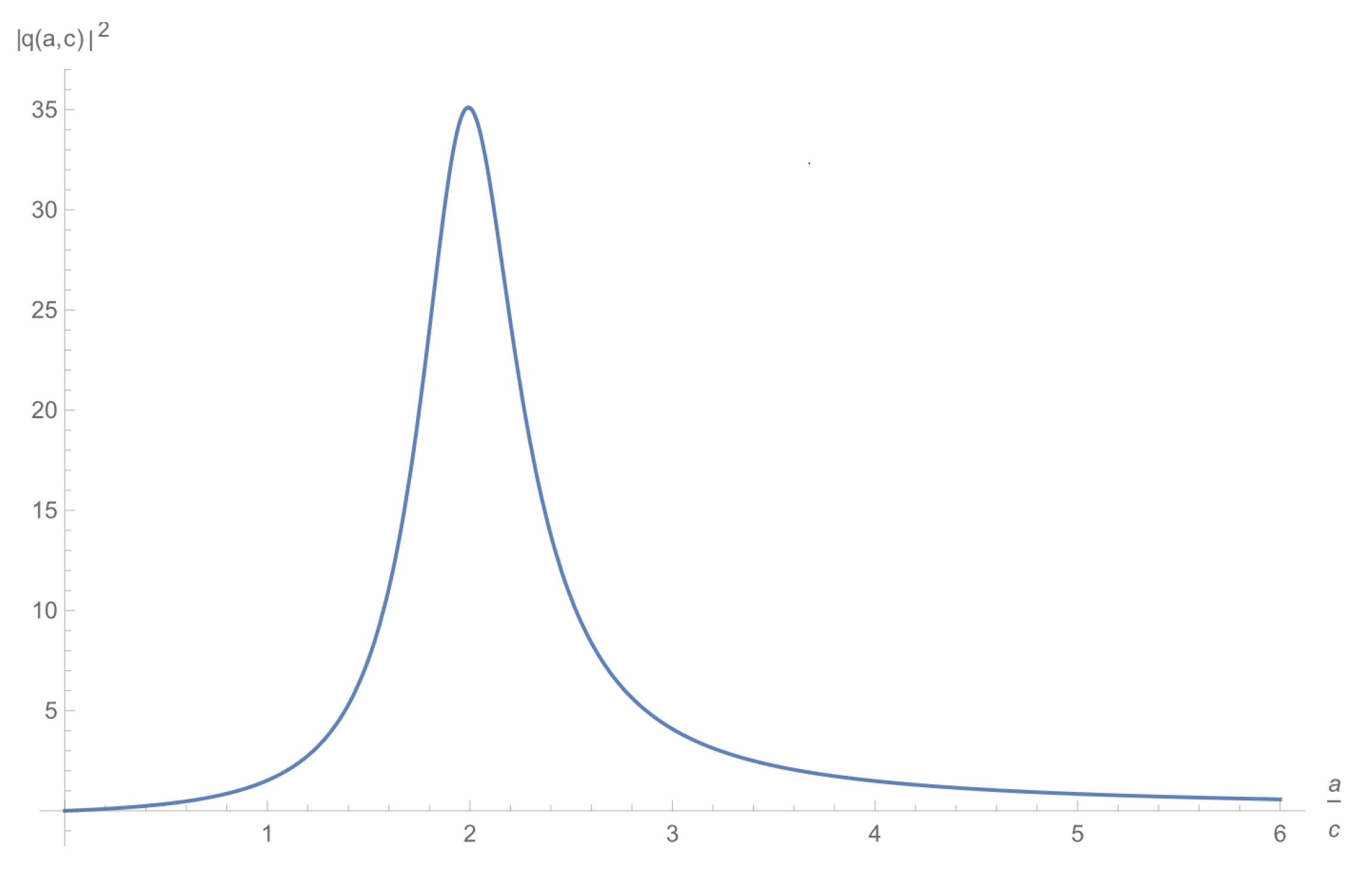
Figure 2 describes this function. The peak in this function reflects how the back-action from measuring the photon restricts the final state of the metric; the peak is centered near the expected scale factor proportion given the photon measurement.
2.2. As a Measurement of Scale Factor
One can see from Equation (13) that measuring the photon’s frequency (partially) collapses the metric wavefunction. Consider, the extreme case where and , hence a scaling of . This results in
and
which implies the scale factors scale by s from the initial state. Observe that the final state is still affected by evolution effects, though these effects are trivial for the simple evolution (Equation (15)).
2.3. Multiple Measurements
Consider the case in which multiple photons are emitted and later measured. In particular, say N photons are detected, such that all photons are emitted before any are measured. Assume that some time passes between each emission, measurement, and between the emissions and measurements. Thus, there are total periods of evolution; label these with the functions for . Assume that the photons do not interfere (i.e., they are spatially separated) so we can define , for , to describe the effects of measuring the jth photon; if the photons interfered, we would not be able to separate the ’s into functions that consider only one photon. The wavefunction of the metric after k photon measurements, tracing over photon modes, is
where . Equation (20) reduces to Equation (13) when .
Assume that the metric is approximately static between emissions and between measurements. That is, the metric only evolves between the last emission and first measurement. Then, we can assume for . To make an additional simplification, assume that all the detectors are the same and that all the emitters are the same, i.e., , independent of j. Thus, Equation (20) becomes
for normalization constant . Observe that q, in general, describes a function that peaks around the expected scale factor. Thus, in the limit , acts like a Dirac-delta function of centered around the least suppressed scale factor; i.e., the maximum of q. The scale factor can then be determined to arbitrary accuracy with sufficiently many measurements.
2.4. Classical Dynamics
Metric dynamics are typically described in classical terms, thus it may be useful to describe the dynamics in terms of deviation from classical dynamics. To do this, we can move into a rotating frame in which the classical evolution is “subtracted-out”. For this, it is useful to use the logarithmic scale factor (Equation (7)). Denote the classical (logarithmic) scale factor in conformal time with . Then, define the unitary
for the canonical momentum satisfying .
Starting with the ket, , we define the rotating-frame ket by
The metric evolution (Equation (11)) is then transformed to the rotating frame according to
Using the fact that , we have
where we make the simplifying assumption that is an eigenket of . Thus, the rotating frame describes the “quantum-part” of the metric. If the dynamics are entirely classical, then we would expect trivial dynamics for the quantum-part: .
3. Analogy: Optomechanical Cavity
Direct experimental probes of cosmological expansion are limited due to the spatial and temporal scales involved. However, it may be possible to emulate cosmological processes with accessible experimental apparatus. Such an experiment must possess the same or analogous properties of the cosmology being emulated. For example, one may want to consider a process in which photon redshift occurs: such as Doppler shift, gravitational redshift, and cosmological redshift. Here, we will consider the frequency shift induced in an optical cavity by a variable cavity length.
3.1. Cavity as Space
Consider a Fabry–Pérot interferometer: an optical cavity consisting of two mirrors. The cavity only permits integral frequencies,
where n is some positive integer (the frequency mode), c is the speed of light, and L is the length of the cavity. Typically, the cavity is populated by only one mode, denoted simply , when e.g., the free spectral range is large. This is because a source will populate the cavity by supplying a bandwidth of frequencies much smaller than the free spectral range of the cavity around .
If the position of one of the mirrors is classically fixed while the other is allowed to move (within some potential), the optical cavity becomes coupled to the mechanical motion of the second mirror. This is seen in which is dependent on the length of the cavity. Choosing coordinates where the fixed mirror is at , the Hamiltonian of the system becomes
where and are the operators associated with the position and momentum of the mirror’s mechanical motion, and and are the annihilation and creation operators of the mode (subscript n sometimes omitted for single-mode case). If additional modes are present in this system, one would sum over n on the first term for all possible modes. The energy associated with the mechanical system (with mass M) is given by . Observe that the singularity at is avoided, because this is associated with a zero-length cavity. A harmonic oscillator is often used for the mechanical system (such as a mirror on a spring) due to its symmetry with the optical modes and experimental realization (for a review of optomechanical cavities, see, e.g., ref. [27]). However, we will consider a general mechanical potential that may or may not include harmonic terms. For much of this analysis, we find the case of freely moving mirrors sufficiently complex to enable intriguing analogies. In practice, a freely moving mirror can be well approximated by a mirror on a spring with a low stiffness, conditional on the dynamics of the experiment occur much faster than the nominal resonance frequency of the mirror’s motion.
Motivated by the FRW universe, consider defining the scaling operator
for an arbitrarily chosen position . Likewise define to obey the canonical commutation relation, . Now, if a physical can be chosen such that the evolution of the analogy system is consistent with that of the (FRW) universe, this system can be experimentally explored.
In the Heisenberg picture, solving for the evolution of the and operator yields:
where . The dot, , denotes the derivative in (coordinate) time. Combining these equations, and noting the commutation relation , yields the equation of motion
Consider the simple case of a free mirror (i.e., ). Then for a cavity with N photons—assume to avoid trivial case. Observe that, regardless of initial conditions, this corresponds to an (eventually) expanding cavity. After a long time, the mirror will move outward at a constant velocity. One can think of this as radiation pressure pushing the mirrors apart. As the mirrors separate, the cavity frequency decreases. Thus there is less pressure on the mirror. Eventually, the mirror will move at an approximately constant velocity, as if no longer being accelerated by the low-energy photons. Observe that the redshift and period of the photon traversing the cavity each contribute a factor to the acceleration of the mirror, hence . As with the FRW model, the presence of radiation drives the dynamics of the system.
In this single-cavity construction, the cavity can be thought of as the space through which light travels. A source populates the cavity with a given (“coordinate”) frequency. The photons populate the cavity for some time at the same cavity mode (“conformal frequency”) then are emitted to a detector. The detector may measure a different frequency than what the source output, as the cavity frequencies change. Measuring the shift from the emitted to the detected frequency yields information on how the cavity position changed. The choice in mechanical potential determines the dynamics of the system.
Various connections can be made between the tFRW cosmology and optomechanical system described here. The coordinate frequency (analogy) of the cavity is , which scales correctly with the scale factor (analogy), . The conformal frequency is analogous to the cavity mode n—a constant quantity associated with a traversing photon that is essentially inaccessible to an observer that cannot measure the mirror position (scale factor) directly. Equivalently, one can define as the analogous conformal frequency.
Observe that the evolution of the metric is described in terms of the optomechanical equations of motion instead of the reverse. Thus, one wants to start with a model for cosmological equations of motion then choose an optomechanical system that can mimic these equations. The optomechanical system is modified via the potential on the mechanical system, .
3.2. Cavities as Atoms
Consider a system with two coupled cavities (see Figure 3). In this system, two cavities each share a mechanical coupling on one mirror. The other two mirrors are classically fixed, though not necessarily at the same relative position. The cavities are also allowed to transfer photon modes. In this analogy, the cavities will be shown to behave like atoms in the tFRW model.
In this optomechanical system, one cavity (say the upper cavity) can serve as a source, while the other (lower cavity) serves as the detector. The cavity frequency is analogous to the conformal frequency while the cavity mode is analogous to the coordinate frequency. Thus, the emission spectrum of the cavities is constant with respect to cavity modes (as with the coordinate frequency wavepackets in Equations (9) and (10)). The shared mechanical mode reflects the metric wavefunction.
Consider a process in which a photon is emitted by the upper cavity, the cavities are allowed to shrink, then the photon is absorbed by the lower cavity. The lower cavity would see a redshifted photon in this process as the respective cavity modes increase in frequency, while the en route photon frequency is constant. This could be thought of as atoms appearing “smaller” as the universe expands. We remark here that the reverse process (detector to source) is in principle allowed both in the real universe and our toy model, but we will assume no emission from the detector cavity at present. Crucially, we assume a relatively long delay (larger than the inverse linewidths of the cavities) for the photon path that exits one cavity and enters the other.
Denote the frequency in the cavities as for and refer to the relative positions of the fixed mirrors to the equilibrium position of the moving mirrors. As defined, yields a position relative to the mechanical equilibrium. Considering the energy from the photons in the cavities,
where are the respective annihilation operators.
We note that this equation, as stands, will not be able to explore a wide range of redshifts. However, we can do substantially better by moving to a rotating frame, e.g., by having a weak, narrowband thermal or coherent source at a frequency coming into the source cavity. More specifically, the simplest example would be a series of excited, broad linewidth atoms near the cavity frequency in the Purcell-enhanced regime, such that photon emission occurs preferentially at the cavity frequency. A more interesting option for sources for future experiments might include having an induced chemical potential for light using parametric coupling to a bath [28]. On the detector side, we can consider putting a broadband photodetector on the transmitting side of the detector cavity.
3.3. Hubble Expansion in the Rotating Frame
In the cavities-as-atoms picture, we can move to a rotating frame according to the unitary transformation . Then, performing a linear expansion about small displacements of the cavity modes gives:
where , and is the detuning for . We assume that for the entire range of dynamics that follows to maintain a semblance of physicality for our model.
We now examine the spectrum of emission and absorption, as defined in Equations (9) and (10). The cavity resonance should move with scale factor according to , where is chosen to reflect . Thus, we can define the optomechanical scale factor according to
which can be written as
Observe that the allowed Hilbert space is restricted such that because the mechanical mirror cannot move past the fixed mirror.
Applying this change-of-variables to Equation (33) yields
From this hamiltonian, we would like to emulate the frequency scaling described in Equation (3). This can be achieved by demanding the first term in the above hamiltonian vanish. To achieve this, the constraint is applied to the system. That is, freely choose, say, and set as the rotating frame frequencies. Now, we can set to be independent of k. Then, the optical part of the hamiltonian is simply
where each cavity has, in the rotating frame, an effective ‘atomic’ frequency
Connecting to the tFRW model, is analogous to the coordinate frequency wavepacket (single-valued in this scenario) in Equations (9) and (10).
Consider the dynamics of this system. It is first useful to consider the Hubble parameter as defined in cosmology
Thus, the conformal time derivative of from Equation (35) (taking as the analogous scale factor) can be written
Observe that, in this analogy, the time is conformal time because the photon traverses between the cavities at constant frequency. Conventionally, the Hubble parameter is approximated as a constant. With this assumption, the above dynamics implies that the mirror has constant velocity, or that the mirror’s motion is free. A free mirror in the system can be obtained by considering short time scales while the mirror is near equilibrium position so that the mirror has negligible acceleration.
Speaking more practically, we can now consider the following experiment: a photon is created in the source cavity, then detected at a later time at the detector cavity. If we start with a combined wavefunction of the source, detector, and mirror of the form , the post-selected wavefunction after the detection has selected a narrow range of allowed a values, according to . At the same time, the intuitive explanation—that detection yields information about the position of the mirror—explains the same experiment. Thus by looking for the position-based dephasing of the mirror using weak homodyne measurement of the mirror quadratures, one can estimate this ‘cosmological analog’ decoherence.
3.4. Logarithmic Scale-Factor
We present here methods to describe the previous optomechanical analogies in terms of the logarithmic scale factor (Equation (7)). In some sense, this is a trivial (albeit possibly cumbersome) calculation as one can simply apply the defining homeomorphism to alternate between the two scale factors. To make the problem more interesting, we would like to consider a different type of optomechanical system than the conventional cavtity. In particular, we may consider one in which the coupling term is given by
This describes an optical system at resonance in which a mechanical mode evanescently modifies the energy of the system. The exponential term is a natural choice when dealing with a logarithmic scale factor. Moreover, this Hamiltonian has experimental potential [29,30,31].
First, we look at the single-system case. Still treating the mechanical system as controlling the metric, we would like the optical term to be of the form where is the analogous logarithmic scale factor. The obvious choice is then to define
Adding the mechanical terms and moving into a rotating frame with the unitary to eliminate the resonance term, we obtain the full Hamiltonian:
which is of the appropriate form—observe that g now fulfills the role of .
Next, we would like to consider the two-system analogy. To couple the systems, we will assume that they share the same . Moreover, to simplify the problem, we will assume that the evanescent couplings have the same characteristic length, , though the coupling strengths g may be different. As before, we move into a rotating frame with the unitary, . Labeling the systems with the rotating-frame optical Hamiltonian is then
Desiring the relationship (so occurs at ), we obtain
which can be written as
Taking Equation (46) and using Equation (44) yields
Demanding, then, that the first term vanishes, we have for all k. As before, this is simply a constraint on one’s choice of when moving to the rotating frame. Finally, we have a Hamiltonian of the appropriate form,
for the effective frequency,
Consider the Hubble Equation (39). In terms of the logarithmic scale factor in conformal time, this is given by . Using Equation (45) yields the dynamics
A system following these dynamics will mimic the behaviour of an FRW metric undergoing Hubble expansion. Observe that is bounded above by due to the heat death of the universe, hence it is reasonable to assume that and consider only the first lower-order terms. That is, we can consider a free particle with velocity . We recover again a mapping of free particle evolution to expansion of the universe.
4. Conclusions
A toy FRW quantum cosmology was proposed in which a metric variable was treated as a quantum variable. The scale factor in the tFRW model was promoted to the quantum operator , and a metric wavefunction was defined as a superposition of scale factor eigenstates. In this construction, it is natural to describe events in terms of conformal time, . In particular, the photon modes were defined by their conformal frequency in lieu of their coordinate frequency. In doing so, the photon wavefunction is invariant upon time evolution, while a process that generates/annihilates a photon gains a time-dependence via a coupling to the time-dependent scale factor.
A simple process in which a photon is emitted then measured is described. The act of measurement restricts the possible values of the universe scale factor such that the measured redshift agrees with the change in scale factor. The metric becomes entangled with the photon resulting in a wavefunction collapse upon measurement. As photons are constantly being measured throughout the universe, one would expect the scale factor to behave classically—in agreement with observation. This is one potential explanation for the apparent classical behavior of the universe at large scales, though we anticipate that photons are the least entangling aspects of the problem. In this sense, our approach will heavily underestimate actual entanglement between the metric and matter/energy.
Motivated by the toy cosmology, two optomechanical analogies were proposed to emulate the cosmology. In these analogies, a mechanical system serves as the expanding universe. Optical modes couple to the mechanical system and experience frequency shifts analogous to cosmological redshift. Measuring a photon from the system induces a particular, measurable back-action on the system, providing a lower bound on potential decoherence mechanisms for the mirror system. Thus, if we can observe such back-action, the system may help elucidate our cosmological analogy.
The analogies provided approach cosmological scaling in different ways. In the analogy in which the cavity was treated as the space through which photons traveled, the dynamics of the system are most immediately described in terms of coordinate time. That is, the en route photons’ frequency shifts directly as the mechanical system evolves. In contrast, when treating cavities as atoms, the dynamics are described in terms of conformal time, because the en route photons remain static while the cavity modes shift. In either case, there is some freedom to adjust the system to reflect various cosmological dynamics (e.g., consider Equations (31) and (40)). With further considerations, these optomechanical systems may be used to provide a testbed for experiments in quantum cosmology.
Acknowledgments
We thank G. Milburn, S. Jordan for helpful discussions. Funding comes from the NSF funded MRSEC at Princeton University and the NSF funded Physics Frontier Center at the JQI.
Author Contributions
J.M.T. conceived and guided the project; J.A.S. performed the analytical and numerical analysis; J.A.S. and J.M.T. both wrote the paper.
Conflicts of Interest
The authors declare no conflict of interest.
References
- Bojowald, M. Quantum cosmology: A review. Rep. Prog. Phys. 2015, 78, 023901. [Google Scholar] [CrossRef] [PubMed]
- Hubble, E. A relation between distance and radial velocity among extra-galactic nebulae. Proc. Natl. Acad. Sci. USA 1929, 15, 168–173. [Google Scholar] [CrossRef] [PubMed]
- Sitter, W.D. On the Distances and Radial Velocities of Extra-Galactic Nebulae, and the Explanation of the Latter by the Relativity Theory of Inertia. Proc. Natl. Acad. Sci. USA 1930, 16, 474–488. [Google Scholar] [CrossRef] [PubMed]
- Bardeen, J.M.; Steinhardt, P.J.; Turner, M.S. Spontaneous creation of almost scale-free density perturbations in an inflationary universe. Phys. Rev. D 1983, 28, 679–693. [Google Scholar] [CrossRef]
- Kibble, T.W.B. Some implications of a cosmological phase transition. Phys. Rep. 1980, 67, 183–199. [Google Scholar] [CrossRef]
- Nelson, E. Quantum decoherence during inflation from gravitational nonlinearities. J. Cosmol. Astropart. Phys. 2016, 2016, 022. [Google Scholar] [CrossRef]
- Özer, M. Implications of a qunatum mechanical treatment of the universe. Mod. Phys. Lett. A 1998, 13, 347–351. [Google Scholar] [CrossRef]
- Hu, B.L.; Matacz, A. Quantum Brownian motion in a bath of parametric oscillators: A model for system-field interactions. Phys. Rev. D 1994, 49, 6612–6635. [Google Scholar] [CrossRef]
- Calzetta, E.; Hu, B.L. Noise and fluctuations in semiclassical gravity. Phys. Rev. D 1994, 49, 6636–6655. [Google Scholar] [CrossRef]
- Alvarenga, F.G.; Batista, A.B.; Fabris, J.C.; Gonçalves, S.V.B. Troubles with Quantum Anisotropic Cosmological Models: Loss of Unitarity. Gen. Relativ. Gravit. 2003, 35, 1659–1677. [Google Scholar] [CrossRef]
- Ren, J.; Meng, X.H.; Zhao, L. Hamiltonian formalism in Friedmann cosmology and its quantization. Phys. Rev. D 2007, 76, 043521. [Google Scholar] [CrossRef]
- Majumder, B. Quantum scalar-metric cosmology with Chaplygin gas. Phys. Lett. B 2011, 697, 101–106. [Google Scholar] [CrossRef]
- Bouhmadi-López, M.; Moniz, P.V. FRW quantum cosmology with a generalized Chaplygin gas. Phys. Rev. D 2005, 71, 063521. [Google Scholar] [CrossRef]
- Khvedelidze, A.M.; Palii, Y.G. Generalized Hamiltonian dynamics of Friedmann cosmology with scalar and spinor matter source fields. Class. Quantum Grav. 2001, 18, 1767–1786. [Google Scholar] [CrossRef]
- Altamirano, N.; Corona-Ugalde, P.; Khosla, K.; Mann, R.B.; Milburn, G. Emergent dark energy via decoherence in quantum interactions. arXiv, 2016; arXiv:1605.05980. [Google Scholar]
- Zurek, W.H. Cosmological experiments in superfluid helium? Nature 1985, 317, 505–508. [Google Scholar] [CrossRef]
- Zurek, W.H. Cosmological experiments in condensed matter systems. Phys. Rep. 1996, 276, 177–221. [Google Scholar] [CrossRef]
- Steinhauer, J. Observation of quantum Hawking radiation and its entanglement in an analogue black hole. Nat. Phys. 2016, 12, 959–965. [Google Scholar] [CrossRef]
- Matos, T.; Gomez, E. Space-time curvature signatures in Bose–Einstein condensates. Eur. Phys. J. D 2015, 69, 125. [Google Scholar] [CrossRef]
- Cortijo, A.; Vozmediano, M.A.H. Electronic properties of curved graphene sheets. Europhys. Lett. EPL 2007, 77, 47002. [Google Scholar] [CrossRef]
- Szpak, N. Curved spacetimes in the lab. arXiv, 2014; arXiv:1410.1567. [Google Scholar]
- Tian, Z.; Jing, J.; Dragan, A. Analog cosmological particle generation in a superconducting circuit. Phys. Rev. D 2017, 95, 125003. [Google Scholar] [CrossRef]
- Tsagas, C.G. Electromagnetic fields in curved spacetimes. Class. Quantum Grav. 2005, 22, 393–407. [Google Scholar] [CrossRef]
- Bonnor, W.B. Size of a hydrogen atom in the expanding universe. Class. Quantum Grav. 1999, 16, 1313–1321. [Google Scholar] [CrossRef]
- Nowotny, E. Hydrogen atom in the Friedman universe. Commun. Math. Phys. 1972, 26, 321–332. [Google Scholar] [CrossRef]
- Berman, P.R.; Ford, G.W. Spectrum in spontaneous emission: Beyond the Weisskopf-Wigner approximation. Phys. Rev. A 2010, 82, 023818. [Google Scholar] [CrossRef]
- Aspelmeyer, M.; Kippenberg, T.J.; Marquardt, F. Cavity optomechanics. Rev. Mod. Phys. 2014, 86, 1391–1452. [Google Scholar] [CrossRef]
- Hafezi, M.; Adhikari, P.; Taylor, J.M. Chemical potential for light by parametric coupling. Phys. Rev. B 2015, 92, 174305. [Google Scholar] [CrossRef]
- Kim, P.H.; Doolin, C.; Hauer, B.D.; MacDonald, A.J.R.; Freeman, M.R.; Barclay, P.E.; Davis, J.P. Nanoscale torsional optomechanics. Appl. Phys. Lett. 2013, 102, 53102–53105. [Google Scholar] [CrossRef]
- Eichenfield, M.; Chan, J.; Camacho, R.M.; Vahala, K.J.; Painter, O. Optomechanical crystals. Nature 2009, 462, 78–82. [Google Scholar] [CrossRef] [PubMed]
- Ghulinyan, M.; Ramiro-Manzano, F.; Prtljaga, N.; Guider, R.; Carusotto, I.; Pitanti, A.; Pucker, G.; Pavesi, L. Oscillatory Vertical Coupling between a Whispering-Gallery Resonator and a Bus Waveguide. Phys. Rev. Lett. 2013, 110, 163901. [Google Scholar] [CrossRef] [PubMed]
Figure 1.
The Friedmann–Robertson–Walker–Lemaître (FRW) for an exponentially expanding universe in (a) coordinate and (b) conformal time. Blue vertical lines are separated by one unit of proper distance, while horizontal lines are separated by one unit of proper time. The universe is populated by comoving particles (black disks) which exchange a photon. Color is used to emphasize which frequencies shift.
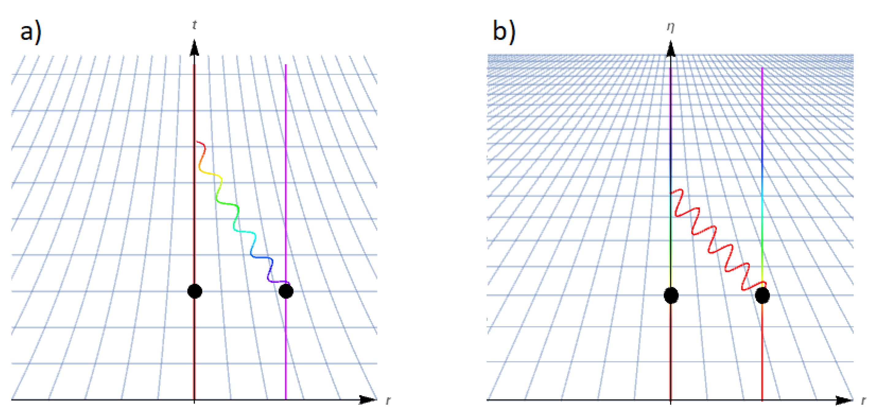
Figure 2.
The result of for the simple example with the Lorentzian wavefunctions. Here, , , and .

Figure 3.
A schematic of the coupled two-cavity system. Mirrors to the left of the cavities enable photons to transfer between cavities. The right cavity mirrors share a coupling to a mechanical system (denoted as a spring in the schematic). In addition, the top mirror is driven by a source, while the bottom mirror has an attached detector.

© 2017 by the authors. Licensee MDPI, Basel, Switzerland. This article is an open access article distributed under the terms and conditions of the Creative Commons Attribution (CC BY) license (http://creativecommons.org/licenses/by/4.0/).
Share and Cite
MDPI and ACS Style
Smiga, J.A.; Taylor, J.M. Optomechanical Analogy for Toy Cosmology with Quantized Scale Factor. Entropy 2017, 19, 485. https://doi.org/10.3390/e19090485
AMA Style
Smiga JA, Taylor JM. Optomechanical Analogy for Toy Cosmology with Quantized Scale Factor. Entropy. 2017; 19(9):485. https://doi.org/10.3390/e19090485
Chicago/Turabian StyleSmiga, Joseph A., and Jacob M. Taylor. 2017. "Optomechanical Analogy for Toy Cosmology with Quantized Scale Factor" Entropy 19, no. 9: 485. https://doi.org/10.3390/e19090485
Note that from the first issue of 2016, this journal uses article numbers instead of page numbers. See further details here.