Objective Weights Based on Ordered Fuzzy Numbers for Fuzzy Multiple Criteria Decision-Making Methods

Faculty of Computer Science, Bialystok University of Technology, 15-351 Bialystok, Poland
Entropy 2017, 19(7), 373; https://doi.org/10.3390/e19070373
Submission received: 7 June 2017
/
Revised: 16 July 2017
/
Accepted: 20 July 2017
/
Published: 21 July 2017
(This article belongs to the Section Information Theory, Probability and Statistics)
Abstract
:Fuzzy multiple criteria decision-making (FMCDM) methods are techniques of finding the trade-off option out of all feasible alternatives that are characterized by multiple criteria and where data cannot be measured precisely, but can be represented, for instance, by ordered fuzzy numbers (OFNs). One of the main steps in FMCDM methods consist in finding the appropriate criteria weights. A method based on the concept of Shannon entropy is one of many techniques for the determination of criteria weights when obtaining them from the decision-maker is not possible. The goal of the paper is to extend the notion of Shannon entropy to fuzzy data represented by OFNs. The proposed approach allows to obtain criteria weights as OFNs, which are normalized and sum to 1.
1. Introduction
Fuzzy multiple criteria decision-making (FMCDM) methods are techniques used to find the trade-off option out of all feasible alternatives that are characterized by multiple criteria and when data cannot be measured precisely. In such situations the ratings of alternatives and the criteria weights, whose evaluations are based on unquantifiable, incomplete, or unobtainable information, are usually expressed by interval numbers [1,2,3] or fuzzy numbers (convex fuzzy numbers—CFNs) [4,5,6]. A new approach consists in using an FMCDM method based on ordered fuzzy numbers (OFNs) which are well suited to handle incomplete and uncertain knowledge and information.
This new approach to multiple criteria decision support has been considered, so far, in a few papers only [7,8,9]. The first application of OFNs for the FMCDM method was presented at the Sixth Podlasie Conference on Mathematics in Bialystok, Poland [7] by Kacprzak and Roszkowska, and discussed in detail in [8]. In that paper, the authors evaluated alternatives with respect to criteria using linguistic expressions, in which linguistic terms were quantified on a scale given in advance. The scale was extended to include intermediate values, such as “more than 2” or “less than 3”, which were expressed by trapezoidal OFNs, together with “2” and “3”. The additional property of OFNs (i.e., orientation) was used to include information about the type of criteria (benefit or cost). The authors showed that the Fuzzy Simple Additive Weighting (FSAW) and Fuzzy Technique for Order of Preference by Similarity to Ideal Solution (FTOPSIS) methods based on OFNs can better distinguish alternatives as compared with classical Simple Additive Weighting (SAW) and Technique for Order of Preference by Similarity to Ideal Solution (TOPSIS) methods, which used crisp values, and with FSAW and FTOPSIS, which used classical fuzzy numbers. The FTOPSIS method with OFNs has also been used in solving a real-life problem of discrete flow control in a manufacturing system [9]. The authors have tested the FTOPSIS method with OFNs in a flow control system and compared it to the classical TOPSIS method and to other simple control methods. As a result, they concluded that FTOPSIS with OFNs is better suited for the analysed case than the classical TOPSIS or than most other methods considered.
One of the main steps in FMCDM methods is the determination of the appropriate weights (the relative importance) of the criteria, because of their significant impact on the final result. Since each criterion has a different meaning, we cannot assume that all of them are equally important [10,11]. In the literature, various methods to determine criteria weights have been proposed. Most of them can be classified into two categories: subjective and objective weights, depending on the information provided. Subjective weights are determined according to the preferences or judgments of the decision-makers only and can reflect the subjectivity of their knowledge and experience. This category includes: the eigenvector method [12], the weighted least square method [13], the Delphi method [14], and others. Objective weights are determined by solving mathematical models. They disregard subjective preferences or judgments of the decision-makers; instead, they are based on objective information (e.g., decision matrix). This category includes the entropy method [15], multiple objective programming [16], and others.
Most of FMCDM applications to real-life problems use only subjective weights. However, when it is not possible to obtain reliable subjective weights, objective weights become useful [17]. One of the methods of obtaining objective weights applies the notion of Shannon entropy mentioned before. Moreover, let us note that it is reasonable and logical that when ratings of alternatives with respect to criteria are imprecise, as is the case in FMCDM methods, the weights of criteria should also be imprecise. Therefore, Shannon entropy should be extended to imprecise Shannon entropy.
Applications of Shannon entropy to the determination of weights in FMCDM problems have been discussed in the literature. One of the approaches is based on the characterization of a fuzzy number by its -levels and by an extension of Shannon entropy to interval data [2]. The main limitation of this approach is that the obtained weights do not have to preserve the property that their ranges belong to [0, 1] (but can be normalized) and they do not sum up to 1. Moreover, the empirical example with five levels {0.1, 0.3, 0.5, 0.7, 0.9} has shown that the rankings for different α-levels can be different. The authors have concluded that the overall ranking of the criteria cannot be easily determined. Another approach to the determination of weights in FMCDM problems uses the concept of defuzzification [6,18,19,20]. This relies on the conversion of fuzzy numbers into real numbers; afterwards, the classical Shannon entropy is used. In this approach, during defuzzification, we can lose some important information, such as symmetry, width of the support and kernel, location on the axis of the fuzzy number, etc. Moreover, in the literature we can find many methods of defuzzification of fuzzy numbers and OFNs. Different defuzzification methods can, therefore, generate different rankings of criteria and their relative importance.
The main goal of this paper is to extend the concept of Shannon entropy, using OFNs, which avoid the aforementioned drawbacks. The proposed approach allows to obtain the weights of criteria in the form of OFNs which are normalized and sum to 1. Moreover, several theorems concerning important mathematical properties resulting from the proposed approach, as well as numerical simulations, are presented. An illustrative example will show that the proposed approach based on OFNs gives the same ranking of weights for various α-levels, while the approach from [2] (with fuzzy numbers) results in a ranking that can change from one α-level to another.
The rest of the paper is organized as follows: In Section 2 we introduce basic definitions and notations of OFNs. In Section 3 we present the proposed method of determination of criteria weights using extended Shannon entropy based on OFNs. A simple numerical example is shown in Section 4. In Section 5 presents a comparison of the proposed approach with an approach using fuzzy numbers. Conclusions end the paper.
2. Ordered Fuzzy Numbers
In this section, some definitions related to OFNs used in the paper are briefly presented. The model of ordered fuzzy numbers (OFNs) was introduced and developed by Kosiński and his two co-workers, Prokopowicz and Ślęzak, in 2002 in a series of papers [21,22,23,24]. In our paper, we use the term “ordered fuzzy numbers” which was proposed by Professor Kosiński and his colleagues Prokopowicz and Ślęzak in 2002. After the death of Professor Kosiński, to commemorate and honour him, these numbers are often called “Kosinski fuzzy numbers” [25]. Arithmetic operations in this model are similar to the operations on real numbers, which are a special case of OFNs.
The set of all OFNs will be denoted by . The elements of the OFN are called: , the up part, and , the down part. To conform with the classical notation of fuzzy numbers, the independent variable of both functions and will be denoted by , while their values, by (Figure 1a). The continuity of both functions and implies that their images are bounded intervals, called and , respectively (Figure 1a). Their endpoints will be described as follows: and .
In general, the functions and of the OFN need not be invertible as functions of the variable ; only continuity is required in Definition 1. However, if we assume, additionally, that [24]: (A1) is increasing and is decreasing, (A2) (pointwise), we can define the membership function of the OFN as follows (Figure 1b):
If the functions and/or are not invertible or assumption (A2) is not satisfied, we can obtain so-called improper OFNs (Figure 2). Instead of the membership function, we can then define the membership curve (or relation) in the -plane, consisting of the functions and (as functions of the variable ) and a segment of the line over the interval . Moreover, let us note that in general does not have to be smaller than (Figure 2), in which case we can obtain improper intervals for and/or (discussed in the context of extended interval arithmetic by Kaucher [27]).
Figure 1c shows an OFN as a fuzzy number in the classical meaning (as a convex fuzzy number). Its membership function has an extra arrow denoting the orientation of the OFN, e.g., the order of the inverse functions and . The pair of continuous functions determines a different OFN than the pair . Figure 3 shows that although the two curves have an identical shape, the corresponding membership functions determine two different OFNs.
The set of OFNs can be divided into two subsets:
Orientation can be used to present additional information, for example:
- if we describe an object’s speed, orientation tells us whether the object is moving away or towards us;
- if we analyse the total revenue and/or the total cost of a company, orientation can describe the dependence of the current value on the reference value (increasing or decreasing);
- if we apply FMCDM methods, orientation can show the type of the criteria (benefit or cost).
Basic arithmetic operations on OFNs are defined as pairwise operations on their functions and . Let , , and be OFNs. The arithmetic operations: addition , subtraction , multiplication , and division on them are defined in as follows:
where “”{, , , /} and where is defined when and for each .
Since real numbers are a special case of OFNs, they can be represented in as follows. Let and let be the constant function, i.e., for all . Then is the OFN which represents the real number in . Now we can define the multiplication of an OFN by a real number by the formula:
In Equation (1) of the membership function of the OFN there are four characteristic real numbers: , , , and . If the functions and are linear, these four numbers uniquely describe as follows (Figure 4):
The number is called a trapezoidal OFN if (Figure 4) and a triangular OFN if which for simplicity is often written as follows:
A trapezoidal OFN , where is called normalized. The representation of Equations (4) or (5) allows us to quickly perform arithmetic operations on trapezoidal (triangular) OFNs using these characteristic points. Let and be trapezoidal OFNs. The arithmetic operations on these numbers are then defined by the formula:
where .
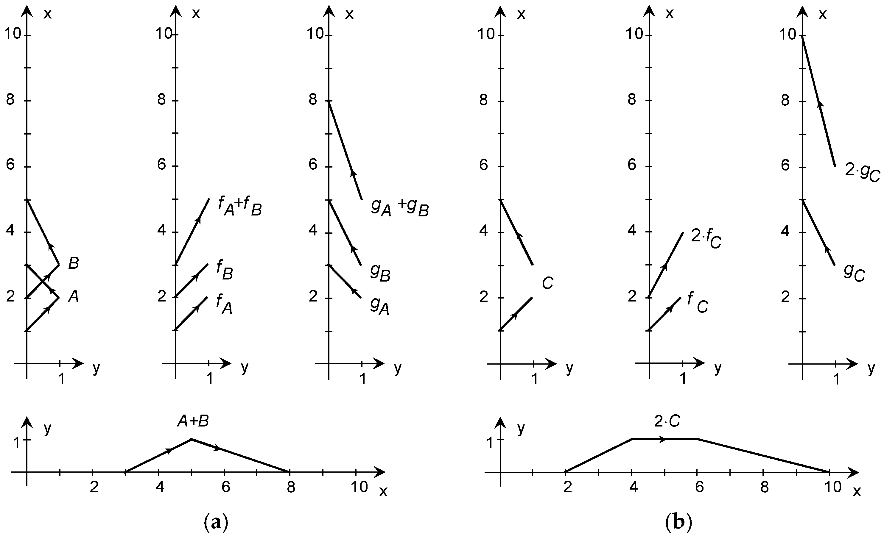
Figure 5a illustrates addition of two triangular OFNs and , and the result , whereas Figure 5b illustrates multiplication of a trapezoidal OFN by a real number and the result .
Defuzzification is a main operation in fuzzy controllers, fuzzy inference systems, and FMCDM methods, which allows to rank OFNs.
Definition 2.
[28]. A map from the space of all OFNs to reals is called a defuzzification functional if it satisfies:
for any and , where represents a crisp number.
Let be an OFN. In , the most frequently used defuzzification methods for are [28]:
- -
- FOM (first of maximum)
- -
- LOM (last of maximum)
- -
- MOM (middle of maximum)
- -
- RCOM (random choice of maximum)
- -
- GM (geometric mean)
- -
- KKCOM (KK choice of maximum)
- -
- COG (centre of gravity)
3. Fuzzy Criteria Weights Based on Fuzzy Shannon Entropy
In this section, we propose an extension of Shannon entropy to a fuzzy environment which will be used to obtain the fuzzy criteria weights for an FMCDM method based on OFNs.
Let us consider a multi-criteria problem which consists of the set of alternatives and the set of criteria . In general, the criteria can be classified into two types: benefit () and cost (). For a benefit criterion, a higher value is better, while for a cost criterion, a smaller value is better. A multi-criteria problem is usually expressed in matrix form, as follows:
where is the rating of the th alternative with respect to the th criterion. Additionally, the relative importance of criteria is given by a vector of weights:
where is the weight of criterion , satisfying the condition .
Most of the MCDM applications to real-life decision-making problems use only subjective weights defined by the decision-maker. However, when it is not possible to obtain reliable subjective weights, objective weights become useful [17]. One of the methods of obtaining objective weights is the application of the concept of Shannon entropy.
Entropy is a term from information theory which is also known as the average (expected) amount of information [29] contained in each criterion (each column of the decision matrix Equation (14)). The greater the value of entropy in a specific criterion, the smaller the differences in the ratings of alternatives with respect to this criterion. This, in turn, means that this criterion provides less information and has a smaller weight. It follows that this criterion becomes less important in the decision-making process.
Let us consider the decision matrix (Equation (14)), where . Then criteria weights can be determined as follows:
- 1.
- Construct the normalized decision matrix , where:
- 2.
- Construct the vector of Shannon entropy , where:and is defined as 0 if .
- 3.
- Calculate the vector of diversification degrees , where:The higher the degree , the more important the corresponding criterion .
- 4.
- Calculate the vector of criteria weights , where:
It is reasonable and logical that when the ratings of alternatives with respect to criteria are represented by OFNs, the weights of criteria should be also represented by OFNs. This means that the concept of Shannon entropy needs to be extended to fuzzy Shannon entropy based on OFNs.
We will present a method of determining the weights of criteria based on OFNs using triangular OFNs (the proposed method can be easily extended to trapezoidal OFNs). The orientation of OFNs will be used to distinguish between types of criteria. Namely, to represent the value of a benefit criterion we use positive triangular OFN , i.e., an OFN such that , while for a cost criterion, negative triangular OFN , i.e., an OFN such that . Then the calculation of criteria weights based on triangular OFNs can be described in the following steps.
- STEP 1:
- Construct the fuzzy decision matrix , where:is the rating of alternative with respect to criterion represented by a triangular OFN.
- STEP 2:
- Construct the normalized fuzzy decision matrix , where:
If, for all we have or or , we define or or to be 0, respectively.
Remark 1:
The orientation of OFNs is used for input data to distinguish between the types of criteria. Let us note that during the calculations using Equation (21) the orientation of the resulting OFNs can change (from positive to negative, and vice versa) and even improper OFNs can occur. This is shown in the numerical example presented below.
Let us consider the following three OFN-rated alternatives with respect to j-th benefit criterion: , , and . The normalized OFNs, calculated using Equation (14), are: , , and . Note that after normalization, has the same orientation as the input data, has the opposite orientation, and is an improper OFN.
- STEP 3:
- Construct the vector of fuzzy Shannon entropy , where:and or or is defined as 0 if or or , respectively.
- STEP 4:
- Calculate the vector of fuzzy diversification , where:
- STEP 5:
- Calculate the vector of fuzzy criteria weights , where:
If for all we have or or , we define or or to be 0, respectively.
Theorem 1.
The criteria weights (Equation (24)) are normalized.
Proof.
Let us note that for all we have , and . Hence, it follows that , , and , which means that . ☐
Theorem 2.
If all the ratings of alternatives with respect to criteria are crisp data then the proposed method of determining the weights of criteria using the fuzzy Shannon entropy based on OFNs leads to the classical method of determining the weights of the criteria using the classical Shannon entropy.
Proof.
Let us note that if all the ratings of alternatives with respect to criteria are crisp data, then in Equation (20) we have and also in Equation (21). This means that from Equation (22) we have and, therefore, in Equation (23). Finally, from Equation (24) we have . ☐
Theorem 3.
If at least one of the ratings of any alternative with respect to any criterion is an OFN, all the criteria weights are also OFNs.
Proof.
Assume that for and we have , which means that is an OFN. Then from Equation (21) we have for all . Next, from Equation (22) we have and from Equation (23) . Finally, from Equation (24) we have for all . ☐
Theorem 4.
The obtained weights from Equation (24) satisfy the condition .
Proof.
From Equation (24) we have:
☐
Theoremf 5.
If all alternatives are evaluated identically with respect to a criterion, for example, th criterion , then .
Proof.
Assume that for each alternative the evaluations with respect to -th criterion are the same and equal to . Therefore, using Equation (21), after the normalization for all , we have . Since and using Equation (22), we have . From Equation (23) we have and from Equation (24) we obtain . ☐
Theorem 6.
If all alternatives are evaluated identically with respect to a criterion, for example, k-th criterion and j-th criterion , e.g., for , then
Proof.
Assume that for each alternative the evaluations with respect to -th criterion and j-th criterion are the same, e.g., for . Then, using Equation (21), we have for and when we calculate the entropy using Equation (22), we obtain . Hence, from Equation (23) we have and, finally, using Equation (24), we obtain . ☐
4. An Illustrative Example
In this section, we present a simple numerical example of the proposed method. Let us consider the multi-criteria problem of selecting a provider of medical equipment to a medical centre. Four bidders , , , and responded to the invitation to bid. They are rated with respect to the following criteria: : price, : length of warranty, : conditions of service, : multifunctionality of the equipment, that is, the capability for extension and modification, : payment term, : comprehensiveness of the offer, that is, training, delivery, installation, and possibility of leasing.
For the ratings of the alternatives with respect to the criteria the linguistic variables from Table 1 are used. The results of the ratings are shown in Table 2. The linguistic variables from Table 2 are converted into triangular OFNs; the corresponding fuzzy decision matrix is presented in Table 3. Next, this matrix is normalized using Equation (21) and presented in Table 4. Based on the data from Table 4 and using Equations (22)–(24), the vector of fuzzy Shannon entropy, the vector of fuzzy diversification, and the vector of fuzzy criteria weights are calculated and shown in Table 5. To determine the ranking of the criteria we can use one of the defuzzification methods of Equations (7)–(13) presented in Section 2. The simplest defuzzification method for triangular OFNs consists in selecting a central value which is equivalent to using one of the Equations (7)–(12). Table 6 presents the results of defuzzification; the last row shows the rank of each criterion .
5. A Comparison of the Proposed Approach with the Approach Based on CFN
In this section, the approach to the determination of fuzzy criteria weights presented in Section 3 is compared with the approach based on fuzzy numbers described in [2]. To show differences in these approaches we use the illustrative example presented in Section 4 and the concept of α-levels. To compare the α-levels and create a ranking of criteria we will use the method proposed by Hu and Wang [30]. This method used another characterization of an -level , using its centre and its radius . Thus, any -level can be written in the form . If is another -level, the method proposed by Hu and Wang can be written as:
and:
Table 7 presents weights and rankings of criteria for selected values of , both for classical fuzzy numbers and for OFNs. Calculations have shown that for CFNs and from 0 to the ranking of criteria is the same, namely . For greater values of the ranking of criteria is different. Starting from the ranking is as follows , which is the same as the ranking presented in Table 6. This shows that, for different values of , different rankings are obtained. It is, therefore, difficult to determine the overall ranking of the criteria. On the other hand, the application of the approach proposed in Section 3 gives the same ranking for , which is compatible with the rankings obtained in Table 7 for CFNs and .
Remark 2.
A fuzzy number can be approximated by a triangular fuzzy number using -levels. Then its central value is determined by setting , while its support is obtained by setting [31].
Using the above remark and the approach proposed in [2], fuzzy numbers representing weights of criteria can be determined. Table 8 presents fuzzy criteria weights , fuzzy criteria weights defuzzified by the centre of gravity (Equation (13)), and the ranking of criteria . The resulting ranking of criteria weights is: ; this is different from the rankings presented in Table 7 for CFNs and for different values . Table 9 presents OFN-based fuzzy criteria weights , fuzzy criteria weights defuzzified by the centre of gravity (Equation (13)), and the ranking of criteria . The obtained ranking of criteria weights is: , compatible with the ranking obtained in Table 6 and Table 7 for OFNs.
6. Conclusions
Considering that in some real-life decision-making problems it is difficult to determine the exact values of the ratings of alternatives and the criteria weights, these values can be expressed as OFNs. Moreover, most FMCDM applications use only subjective weights. However, when it is not possible to obtain reliable subjective weights, objective weights become useful. One of the methods for obtaining objective criteria weights for an MCDM method is a technique based on the concept of Shannon entropy. It is logical that when the ratings of alternatives are represented as OFNs, the criteria weights should be also OFNs.
In this paper, a method for obtaining criteria weights based on the concept of Shannon entropy has been extended to OFNs. The proposed approach allows to obtain, for each criterion, its weight in the form of an OFN. It has also been shown that the obtained criteria weights are normalized and sum to 1. Moreover, when all the ratings of an alternative with respect to the criteria are crisp data, the proposed method leads to the classical method of determining the weights of criteria using the classical Shannon entropy.
Acknowledgments
The author would like to thank the editor of the Entropy journal and the three anonymous reviewers for their valuable comments and suggestions. The author would also like to express his special gratitude to Ewa Roszkowska at the Faculty of Economy and Management, University of Bialystok, Poland for her valuable advice and suggestions. This research was supported by Bialystok University of Technology grant S/WI/1/2016.
Conflicts of Interest
The author declares no conflict of interest.
References
- Jahanshahloo, G.R.; Lotfi, F.H.; Izadikhah, M. An algorithmic method to extend TOPSIS for decision-making problems with interval data. Appl. Math. Comput. 2006, 175, 1375–1384. [Google Scholar] [CrossRef]
- Lotfi, F.H.; Fallahnejad, R. Imprecise Shannon’s Entropy and Multi Attribute Decision Making. Entropy 2010, 12, 53–62. [Google Scholar] [CrossRef]
- Yue, Z. An extended TOPSIS for determining weights of decision makers with interval numbers. Knowl. Based Syst. 2011, 24, 146–153. [Google Scholar] [CrossRef]
- Chen, C.T. Extensions of the TOPSIS for group decision-making under fuzzy environment. Fuzzy Set Syst. 2000, 114, 1–9. [Google Scholar] [CrossRef]
- Jahanshaloo, G.R.; Lotfi, F.H.; Izadikhah, M. Extension of the TOPSIS method for decision-making problems with fuzzy data. Appl. Math. Comput. 2006, 181, 1544–1551. [Google Scholar] [CrossRef]
- Shemshadi, A.; Shirazi, H.; Toreihi, M.; Tarokh, M.J. A fuzzy VIKOR method for supplier selection based on entropy measure for objective weighting. Expert Syst. Appl. 2011, 38, 12160–12167. [Google Scholar] [CrossRef]
- Kacprzak, D.; Roszkowska, E. The application of ordered fuzzy numbers in the SAW procedure. In Proceedings of the Sixth Podlasie Conference on Mathematics, Bialystok, Poland, 1–4 July 2014; pp. 71–72. [Google Scholar]
- Roszkowska, E.; Kacprzak, D. The fuzzy SAW and fuzzy TOPSIS procedures based on ordered fuzzy numbers. Inf. Sci. 2016, 369, 564–584. [Google Scholar] [CrossRef]
- Rudnik, K.; Kacprzak, D. Fuzzy TOPSIS method with ordered fuzzy numbers for flow control in a manufacturing system. Appl. Soft Comput. 2017, 52, 1020–1041. [Google Scholar] [CrossRef]
- Chen, M.F.; Tzeng, G.H.; Ding, C.G. Fuzzy MCDM approach to select service provider. In Proceedings of the 12th IEEE International Conference on Fuzzy System, St. Louis, MO, USA, 25–28 May 2003; pp. 572–577. [Google Scholar]
- Chen, M.F.; Tzeng, G.H. Combing grey relation and TOPSIS concepts for selecting an expatriate host country. Math. Comput. Model. 2004, 40, 1473–1490. [Google Scholar] [CrossRef]
- Saaty, T.L. A scaling method for priorities in hierarchical structures. J. Math. Psychol. 1977, 15, 234–281. [Google Scholar] [CrossRef]
- Chu, A.T.W.; Kalaba, R.E.; Spingarn, K. A comparison of two methods for determining the weights of belonging to fuzzy sets. J. Optim. Theory Appl. 1979, 27, 531–538. [Google Scholar] [CrossRef]
- Hwang, C.L.; Lin, M.J. Group Decision Making under Multiple Criteria: Methods and Applications; Springer: Berlin, Germany, 1987. [Google Scholar]
- Hwang, C.L.; Yoon, K. Multiple Attribute Decision Making: Methods and Applications; Springer: Berlin, Germany, 1981. [Google Scholar]
- Choo, E.U.; Wedley, W.C. Optimal criterion weights in repetitive multicriteria decision-making. J. Oper. Res. Soc. 1985, 36, 983–992. [Google Scholar] [CrossRef]
- Deng, H.; Yeh, C.H.; Willis, R.J. Inter-company comparison using modified TOPSIS with objective weights. Comput. Oper. Res. 2000, 27, 963–973. [Google Scholar] [CrossRef]
- Liu, H.; Kong, F. A new MADM algorithm based on fuzzy subjective and objective integrated weights. Int. J. Inf. Syst. Sci. 2005, 1, 420–427. [Google Scholar]
- Wang, T.C.; Lee, H.D. Developing a fuzzy TOPSIS approach based on subjective weights and objective weights. Expert Syst. Appl. 2009, 36, 8980–8985. [Google Scholar] [CrossRef]
- Ding, J.F. An integrated fuzzy TOPSIS method for ranking alternatives and its application. J. Mar. Sci. Technol. 2011, 19, 341–352. [Google Scholar]
- Kosiński, W.; Prokopowicz, P.; Ślęzak, D. Drawback of Fuzzy Arithmetics-New Intuitions and Propositions; Method Aritifical Intelligence: Gliwice, Poland, 2002; pp. 231–237. [Google Scholar]
- Kosiński, W.; Prokopowicz, P.; Ślęzak, D. Ordered fuzzy numbers. Bull. Pol. Acad. Sci. 2003, 51, 327–338. [Google Scholar]
- Kosiński, W.; Prokopowicz, P.; Ślęzak, D. Calculus with Fuzzy Numbers; Springer: Berlin/Heidelberg, Germany, 2004; pp. 21–28. [Google Scholar]
- Kosiński, W. On fuzzy number calculus. Int. J. Appl. Math. Comput. Sci. 2006, 16, 51–57. [Google Scholar]
- Prokopowicz, P.; Pedrycz, W. The Directed Compatibility between Ordered Fuzzy Numbers-A Base Tool for a Direction Sensitive Fuzzy Information Processing. Artif. Int. Soft Comput. 2015, 9119, 249–259. [Google Scholar]
- Chwastyk, A.; Kosiński, W. Fuzzy calculus with applications. Math. Appl. 2013, 41, 47–96. [Google Scholar]
- Kaucher, E. Interval analysis in the extended interval space IR. Fundam. Numer. Comput. 1980, 2, 33–49. [Google Scholar]
- Kosiński, W.; Wilczyńska-Sztyma, D. Defuzzification and implication within ordered fuzzy numbers. In Proceedings of the IEEE World Congress on Computational Intelligence (WCCI), Barcelona, Spain, 18–23 July 2010; pp. 1073–1079. [Google Scholar]
- Ding, S.; Shi, Z. Studies on Incident Pattern Recognition Based on Information Entropy. J. Inf. Sci. 2005, 31, 497–502. [Google Scholar]
- Hu, B.Q.; Wang, S. A Novel Approach in Uncertain Programming Part I: New Arithmetic and Order Relation for Interval Numbers. J. Ind. Manag. Optim. 2006, 2, 351–371. [Google Scholar]
- Zimmermann, H.J. Fuzzy Set Theory and Applications; Kluwer Academic Publishers: Boston, MA, USA, 2001. [Google Scholar]
Figure 1.
(a) An OFN, (b) an OFN with its membership function, and (c) an arrow denotes the order of the inverted functions and the orientation of OFN.
Figure 1.
(a) An OFN, (b) an OFN with its membership function, and (c) an arrow denotes the order of the inverted functions and the orientation of OFN.

Figure 2.
Improper OFN with a membership curve (or relation) instead of a membership function.
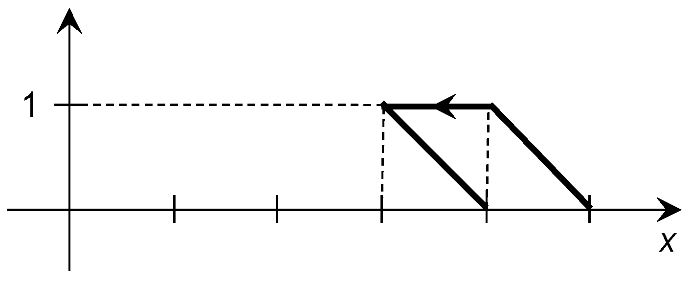
Figure 3.
(a) An OFN with a positive orientation, and (b) an OFN with a negative orientation.
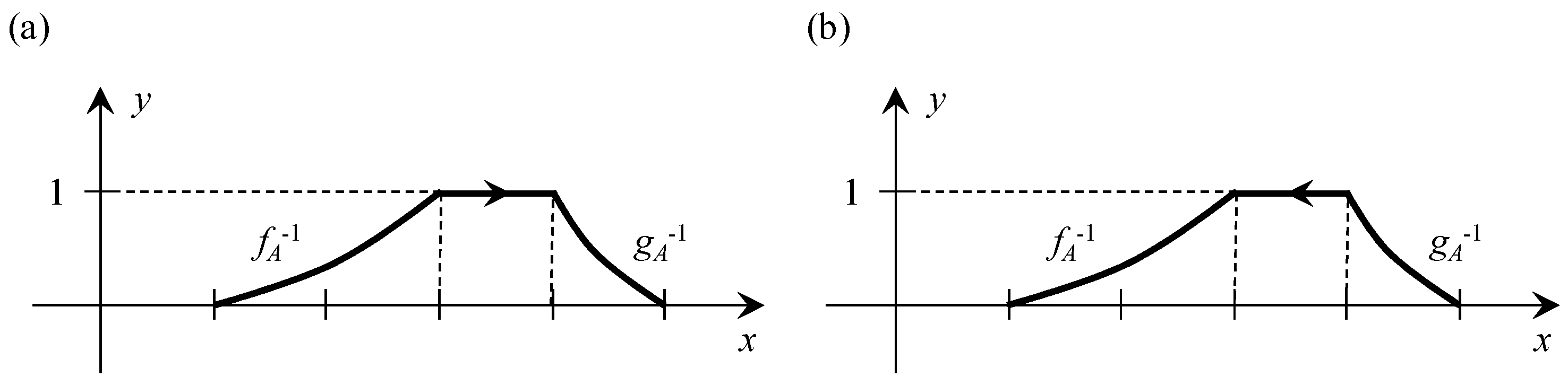
Figure 4.
A trapezoidal OFN (a pair of linear functions) with characteristic points.

Figure 5.
(a) A graphic illustration of addition of two triangular OFNs and , and the result , and (b) a graphic illustration of multiplication of a trapezoidal OFN by a real number and the result
Figure 5.
(a) A graphic illustration of addition of two triangular OFNs and , and the result , and (b) a graphic illustration of multiplication of a trapezoidal OFN by a real number and the result


Table 1.
Linguistic variables for the ratings of the alternatives.
| Linguistic Variables | OFNs for Benefit Criterion | OFNs for Cost Criterion |
|---|---|---|
| Very poor (VP) | (0, 0, 1) | (1, 0, 0) |
| Poor (P) | (0, 1, 3) | (3, 1, 0) |
| Medium poor (MP) | (1, 3, 5) | (5, 3, 1) |
| Fair (F) | (3, 5, 7) | (7, 5, 3) |
| Medium good (MG) | (5, 7, 9) | (9, 7, 5) |
| Good (G) | (7, 9, 10) | (10, 9, 7) |
| Very good (VG) | (9, 10, 10) | (10, 10, 9) |
Table 2.
Decision matrix expressed by linguistic variables.
| Alt. | Criteria | |||||
|---|---|---|---|---|---|---|
| VG | F | G | VG | MG | MG | |
| F | MP | MG | F | F | F | |
| G | MG | G | G | F | MP | |
| MP | MP | VG | G | MG | F | |
Table 3.
Decision matrix expressed by OFNs.
| Alt. | Criteria | |||||
|---|---|---|---|---|---|---|
| (10, 10, 9) | (3, 5, 7) | (7, 9, 10) | (9, 10, 10) | (5, 7, 9) | (5, 7, 9) | |
| (7, 5, 3) | (1, 3, 5) | (5, 7, 9) | (3, 5, 7) | (3, 5, 7) | (3, 5, 7) | |
| (10, 9, 7) | (5, 7, 9) | (7, 9, 10) | (7, 9, 10) | (3, 5, 7) | (1, 3, 5) | |
| (5, 3, 1) | (1, 3, 5) | (9, 10, 10) | (7, 9, 10) | (5, 7, 9) | (3, 5, 7) | |
Table 4.
The normalized decision matrix.
| Alt. | Criteria | |||||
|---|---|---|---|---|---|---|
| (0.313, 0.370, 0.450) | (0.300, 0.278, 0.269) | (0.250, 0.257, 0.256) | (0.346, 0.303, 0.270) | (0.313, 0.292, 0.281) | (0.417, 0.350, 0.321) | |
| (0.219, 0.185, 0.150) | (0.100, 0.167, 0.192) | (0.179, 0.200, 0.231) | (0.115, 0.152, 0.189) | (0.188, 0.208, 0.219) | (0.250, 0.250, 0.250) | |
| (0.313, 0.333, 0.350) | (0.500, 0.389, 0.346) | (0.250, 0.257, 0.256) | (0.269, 0.273, 0.270) | (0.188, 0.208, 0.219) | (0.083, 0.150, 0.179) | |
| (0.156, 0.111, 0.050) | (0.100, 0.167, 0.192) | (0.321, 0.286, 0.256) | (0.269, 0.273, 0.270) | (0.313, 0.292, 0.281) | (0.250, 0.250, 0.250) | |
Table 5.
The vector of fuzzy Shannon entropy— , the vector of fuzzy diversification—, and the vector of fuzzy criteria weights—.
Table 5.
The vector of fuzzy Shannon entropy— , the vector of fuzzy diversification—, and the vector of fuzzy criteria weights—.
| Criteria | ||||||
|---|---|---|---|---|---|---|
| (0.973, 0.931, 0.838) | (0.843, 0.952, 0.977) | (0.985, 0.994, 0.999) | (0.954, 0.978, 0.992) | (0.977, 0.990, 0.994) | (0.913, 0.970, 0.985) | |
| (0.027, 0.069, 0.162) | (0.157, 0.048, 0.023) | (0.015, 0.006, 0.001) | (0.046, 0.022, 0.008) | (0.023, 0.010, 0.006) | (0.087, 0.030, 0.015) | |
| (0.075, 0.376, 0.758) | (0.443, 0.259, 0.107) | (0.042, 0.031, 0.003) | (0.129, 0.117, 0.035) | (0.064, 0.055, 0.026) | (0.247, 0.162, 0.070) | |
Table 6.
Fuzzy criteria weights— , defuzzified fuzzy criteria weights—, and the ranking of criteria—.
Table 6.
Fuzzy criteria weights— , defuzzified fuzzy criteria weights—, and the ranking of criteria—.
| Criteria | ||||||
|---|---|---|---|---|---|---|
| (0.075, 0.376, 0.758) | (0.443, 0.259, 0.107) | (0.042, 0.031, 0.003) | (0.129, 0.117, 0.035) | (0.064, 0.055, 0.026) | (0.247, 0.162, 0.070) | |
| 0.376 | 0.259 | 0.031 | 0.117 | 0.055 | 0.162 | |
| 1 | 2 | 6 | 4 | 5 | 3 | |
Table 7.
Interval criteria weights () and the ranking of criteria () for different α-levels, for CFNs and OFNs.
Table 7.
Interval criteria weights () and the ranking of criteria () for different α-levels, for CFNs and OFNs.
| α | Criteria | CFNs | OFNs | α | Criteria | CFNs | OFNs | ||||
|---|---|---|---|---|---|---|---|---|---|---|---|
| 0.0 | [0.017, 3.380] | 6 | [0.075, 0.758] | 1 | 0.6 | [0.073, 1.050] | 6 | [0.225, 0.537] | 1 | ||
| [0.015, 5.247] | 1 | [0.443, 0.107] | 2 | [0.052, 1.319] | 1 | [0.334, 0.195] | 2 | ||||
| [0.000, 1,548] | 5 | [0.042, 0.003] | 6 | [0.005, 0.359] | 5 | [0.040, 0.017] | 6 | ||||
| [0.005, 1.923] | 4 | [0.129, 0.035] | 4 | [0.022, 0.516] | 4 | [0.136, 0.082] | 4 | ||||
| [0.004, 3.339] | 3 | [0.064, 0.026] | 5 | [0.012, 0.757] | 3 | [0.064, 0.045] | 5 | ||||
| [0.010, 4.433] | 2 | [0.247, 0.070] | 3 | [0.033, 1.071] | 2 | [0.202, 0.124] | 3 | ||||
| 0.2 | [0.026, 2.363] | 6 | [0.114, 0.691] | 1 | 0.8 | [0.142, 0.652] | 5 | [0.297, 0.455] | 1 | ||
| [0.021, 3.525] | 1 | [0.406, 0.134] | 2 | [0.100, 0.675] | 1 | [0.297, 0.227] | 2 | ||||
| [0.001, 1.026] | 5 | [0.043, 0.006] | 6 | [0.010, 0.163] | 6 | [0.036, 0.024] | 6 | ||||
| [0.008, 1.308] | 4 | [0.137, 0.049] | 4 | [0.044, 0.279] | 4 | [0.128, 0.100] | 4 | ||||
| [0.005, 2.213] | 3 | [0.066, 0.032] | 5 | [0.022, 0.331] | 3 | [0.060, 0.050] | 5 | ||||
| [0.014, 2.962] | 2 | [0.234, 0.087] | 3 | [0.063, 0.519] | 2 | [0.183, 0.143] | 3 | ||||
| 0.4 | [0.042, 1.605] | 6 | [0.164, 0.617] | 1 | 0.99 | [0.353, 0.387] | 1 | [0.372, 0.380] | 1 | ||
| [0.032, 2.246] | 1 | [0.370, 0.164] | 2 | [0.243, 0.275] | 2 | [0.261, 0.257] | 2 | ||||
| [0.002, 0.639] | 5 | [0.042, 0.011] | 6 | [0.029, 0.037] | 6 | [0.032, 0.031] | 6 | ||||
| [0.013, 0.850] | 4 | [0.139, 0.065] | 4 | [0.110, 0.124] | 4 | [0.118, 0.117] | 4 | ||||
| [0.007, 1.369] | 3 | [0.066, 0.039] | 5 | [0.052, 0.066] | 5 | [0.055, 0.055] | 5 | ||||
| [0.020, 1,866] | 2 | [0.219, 0.105] | 3 | [0.152, 0.175] | 3 | [0.163, 0.161] | 3 | ||||
Table 8.
CFN-based fuzzy criteria weights , defuzzified (centre of gravity) fuzzy criteria weights , and the ranking of criteria .
Table 8.
CFN-based fuzzy criteria weights , defuzzified (centre of gravity) fuzzy criteria weights , and the ranking of criteria .
| Criteria | ||||||
|---|---|---|---|---|---|---|
| CFN | (0.017, 0.376, 3.380) | (0.015, 0.259, 5.247) | (0.000, 0.031, 1.548) | (0.005, 0.117, 1.923) | (0.004, 0.055, 3.339) | (0.010, 0.162, 4.433) |
| 1.258 | 1.840 | 0.526 | 0.682 | 1.133 | 1.535 | |
| 3 | 1 | 6 | 5 | 4 | 2 | |
Table 9.
OFN-based fuzzy criteria weights , defuzzified (centre of gravity) fuzzy criteria weights , and the ranking of criteria .
Table 9.
OFN-based fuzzy criteria weights , defuzzified (centre of gravity) fuzzy criteria weights , and the ranking of criteria .
| Criteria | ||||||
|---|---|---|---|---|---|---|
| OFN | (0.075, 0.376, 0.758) | (0.443, 0.259, 0.107) | (0.042, 0.031, 0.003) | (0.129, 0.117, 0.035) | (0.064, 0.055, 0.026) | (0.247, 0.162, 0.070) |
| 0.403 | 0.270 | 0.025 | 0.094 | 0.048 | 0.160 | |
| 1 | 2 | 6 | 4 | 5 | 3 | |
© 2017 by the author. Licensee MDPI, Basel, Switzerland. This article is an open access article distributed under the terms and conditions of the Creative Commons Attribution (CC BY) license (http://creativecommons.org/licenses/by/4.0/).
Share and Cite
MDPI and ACS Style
Kacprzak, D. Objective Weights Based on Ordered Fuzzy Numbers for Fuzzy Multiple Criteria Decision-Making Methods. Entropy 2017, 19, 373. https://doi.org/10.3390/e19070373
AMA Style
Kacprzak D. Objective Weights Based on Ordered Fuzzy Numbers for Fuzzy Multiple Criteria Decision-Making Methods. Entropy. 2017; 19(7):373. https://doi.org/10.3390/e19070373
Chicago/Turabian StyleKacprzak, Dariusz. 2017. "Objective Weights Based on Ordered Fuzzy Numbers for Fuzzy Multiple Criteria Decision-Making Methods" Entropy 19, no. 7: 373. https://doi.org/10.3390/e19070373
Note that from the first issue of 2016, this journal uses article numbers instead of page numbers. See further details here.