Content Delivery in Fog-Aided Small-Cell Systems with Offline and Online Caching: An Information—Theoretic Analysis


1
CWiP, Department of Electrical and Computer Engineering, New Jersey Institute of Technology, Newark, NJ 07102, USA
2
Centre for Telecommunications Research, Department of Informatics, King’s College London, London WC2R 2LS, UK
3
Department of Electrical and Computer Engineering, The University of Arizona, Tucson, AZ 85721, USA
*
Author to whom correspondence should be addressed.
Entropy 2017, 19(7), 366; https://doi.org/10.3390/e19070366
Submission received: 28 May 2017
/
Revised: 2 July 2017
/
Accepted: 14 July 2017
/
Published: 18 July 2017
(This article belongs to the Special Issue Network Information Theory)
Abstract
:The storage of frequently requested multimedia content at small-cell base stations (BSs) can reduce the load of macro-BSs without relying on high-speed backhaul links. In this work, the optimal operation of a system consisting of a cache-aided small-cell BS and a macro-BS is investigated for both offline and online caching settings. In particular, a binary fading one-sided interference channel is considered in which the small-cell BS, whose transmission is interfered by the macro-BS, has a limited-capacity cache. The delivery time per bit (DTB) is adopted as a measure of the coding latency, that is, the duration of the transmission block, required for reliable delivery. For offline caching, assuming a static set of popular contents, the minimum achievable DTB is characterized through information-theoretic achievability and converse arguments as a function of the cache capacity and of the capacity of the backhaul link connecting cloud and small-cell BS. For online caching, under a time-varying set of popular contents, the long-term (average) DTB is evaluated for both proactive and reactive caching policies. Furthermore, a converse argument is developed to characterize the minimum achievable long-term DTB for online caching in terms of the minimum achievable DTB for offline caching. The performance of both online and offline caching is finally compared using numerical results.
1. Introduction
Edge or femto-caching relies on the storage of popular multimedia content at small-cell base stations (BSs) of a cellular system. This approach has been widely studied in recent years as a means to deliver video files with reduced latency and limited overhead on backhaul connections to the “cloud” [1,2]. Caching at the edge can be seen as an instance of fog networking, whereby storage, computing and communication capabilities are moved closer to the end users [2]. Edge caching has been initially studied for wireless channel models in which small-cell BSs and macro-BSs cannot coordinate their transmissions and hence cannot cooperatively manage their mutual interference (see [1,2] and references therein). In contrast, recent work in [3,4] addresses the possibility of interference management among edge nodes, such as small-cell and macro-BSs, based on the respective cached contents.
The papers [3,4] proposed caching and transmission schemes that enables coordination and cooperation at the BSs based on the cached contents for a system with three BSs and three users. The performance of these schemes was evaluated in terms of the information-theoretic high signal-to-noise ratio (SNR) metric of the degrees of freedom (DoF), or, more precisely, of its inverse, as a function of the cache capacity of the BSs. More recent research in [5] provided an operational meaning for the inverse of the degrees of freedom metric used in [3,4] in terms of delivery latency, and derived a lower bound on the resulting metric, known as Normalized Delivery Time (NDT), for a general system with any number of BSs and users. The delivery coding latency, henceforth delivery latency, measures the duration of the transmission block. A scenario in which both BSs and users have cache storage is considered in [6,7] under one-shot linear transmission and in [8] under several transmission schemes for both centralized and decentralized caching strategies. It is proved that both BSs and users’ caches have the same quantitative contribution to the achievable sum-DoF. Naderializadeh et al. [9] prop osed a universal scheme for content placement and delivery which is independent of underlying communication networks and is order-optimal in the high-SNR regime. In [10], upper and lower bounds on the NDT of cache-aided MIMO interference channels are provided.
In [11,12] the analysis in [3,4,5] was generalized to study a system in which a cloud server is connected to the BSs via finite-capacity backhaul links and can compensate for partial caching of the library of files at the BSs. This system was referred to as Fog-Radio Access Networks (F-RAN). The minimum NDT latency metric was characterized within a multiplicative factor of 2 in [12] as a function of the cache and backhaul capacity by developing achievability and converse arguments. Other works on NDT characterization include [13,14,15,16]. In [13], a scenario with a multicast fronthaul is studied. In [14], decentralized content placement and file delivery are considered for a F-RAN system with caching at both BSs and users. Reference [15] studies the achievable NDT region to account for heterogenous requirements on the delivery of different files. In [16], the NDT performance of F-RAN systems is considered within a set-up characterized by a time-varying set of popular files. Reference [17] characterized the delivery time per bit of a cache-aided small-cell system by considering binary fading interference channels. Kakar et al. [18] considered the set-up in [17] under linear deterministic channel model to provide upper and lower bounds on the NDT. The optimization of linear processing and often signal processing aspects of F-RAN systems are considered in [19,20,21,22,23].
In this work, we consider the F-RAN model in Figure 1, which includes a small-cell BS and a macro-BS, represented by Encoder 1 and Encoder 2, respectively. The small-cell BS (Encoder 1) is equipped with a cache of finite capacity and can serve a small-cell mobile user, represented by Decoder 1. The macro-BS (Encoder 2) can serve a macro-cell user, namely Decoder 2, as well as, possibly, also Decoder 1. The transmission from the macro-BS (Encoder 2) to Decoder 2 interferes with Decoder 1. It is assumed that the small-cell BS transmits with sufficiently small power so as not to create interference at Decoder 2, which is modeled here as a partially connected wireless channel. We investigate both scenarios with offline and online caching.
The main contributions of this article are as follows:
- An information-theoretic formulation for the analyses of the system in Figure 1 is presented that centers on the characterization of the minimum delivery coding latency measured in terms of the Delivery Time per Bit (DTB), for both offline and online caching. The system model is based on a one-sided interference channel.
- Assuming a fixed set of popular contents, the minimum DTB for the system in Figure 1 is obtained as a function of the cache capacity at Encoder 1 and the capacity of the backhaul link that connects the cloud to Encoder 1 in the offline setting.
- Online caching and delivery schemes based on both reactive and proactive caching principles (see, e.g., [2]) are proposed in the presence of a time-varying set of popular files, and bounds on the corresponding achievable long-term DTBs are derived.
- A lower bound on the achievable long-term DTB is obtained, which is a function of the time-variability of the set of popular files. The lower bound is then utilized to compare the achievable DTBs under offline and online caching.
- Numerical results are provided in which the DTB performance of reactive and proactive online caching schemes is compared with offline caching. In addition, different eviction mechanisms, such as random eviction, Least Recently Used (LRU) and First In First Out (FIFO) (see, e.g., [24]), are evaluated.
The rest of the paper is organized as follows. In Section 2 we present the system model for offline caching, including the definition of the key performance metric of DTB. The minimum DTB for offline caching is then derived and discussed in Section 3. The online caching scenario for the system in Figure 1 is studied in Section 4 in terms of the long-term DTB metric. The comparison between online and offline caching is explored in Section 5. Numerical results are provided in Section 6 and, finally, Section 7 concludes the paper. This work was presented in part in [17].
Notation 1.
Given , we define the set . For any probability p, we define .
2. System Model for Offline Caching
In this section, we study the fog-aided system depicted in Figure 1. We consider a static library of N files denoted by . Each file is independent and identically distributed according to uniform distribution, so that we have , for , where F is the file size in bits. Encoder 1, which models a small-cell BS, has a local cache and is able to store bits. The parameter , with , is hence the fractional cache size and represents the portion of library that can be stored at the cache. Encoder 2, which models a macro-BS, can access the entire library thanks to its direct connection to the cloud. Encoder 1 is also connected to the cloud but only through a rate-limited link of capacity C bits per channel use. We will first consider the scenario of edge-aided offline caching in which , i.e., Encoder 1 does not have access to the cloud, and then extend the analysis to cloud and edge-aided offline caching, i.e., when .
It is assumed that encoders and decoders are connected by a binary fading interference channel, previously studied in [17,25,26]. This model represents a special case of the deterministic linear model of [27] as generalized to account for random fading (see [28]). As illustrated in Figure 1, the signal received at Decoder 1 and Decoder 2 at time t can be written as
where is the vector of binary channel coefficients at time t, and and are the binary transmitted signals from Encoder 1 and Encoder 2, respectively. In (1), all operations are in the binary field. The channel gains are distributed as Bernoulli and Bernoulli, are mutually independent and change independently over time. The parameters and describes the average quality of the communication links originating at Encoder 1 and Encoder 2, respectively, and are hence in practice related to the transmission powers of Encoder 1 and Encoder 2. We remark that a more general model with different erasure probabilities for the links and could also be considered but at the expense of a more cumbersome notation and analysis, which is not further pursued here.
Each user, or decoder, k requests a file from the library at every transmission interval for . The demand vector is defined as . In the next two subsections, we described first the edge-aided scenario and then we generalize it to the cloud and edge-aided system.
2.1. Edge-Aided Offline Caching
The edge-aided small-cell system corresponds to the case with in Figure 1. The system operates according to the following two phases.
- (1)
- Placement phase: The placement phase is defined by functions , at Encoder 1, which maps each file to its cached versionTo satisfy cache storage constraint, it is required thatThe total cache content at Encoder 1 is given byNote that, as in [5,11], we concentrate on caching strategies that allow for arbitrary intra-file coding but not for inter-file coding as per (2). Furthermore, the caching policy is kept fixed over multiple transmission intervals and is thus independent of the receivers’ requests and of the channel realizations in the transmission intervals.
- (2)
- Delivery phase: The delivery phase is in charge of satisfying the given request vector in each transmission interval given the current channel realization. We assume the availability of full Channel State Information (CSI) throughout the transmission block for simplicity of exposition, although this is not required by achievable schemes that will be proven to be optimal (see Remark 1). Note that in practice non-causal CSI for the coding block can be justified for multi-carrier transmission schemes, such as OFDM, in which index t runs over the subcarriers. It is defined by the following two functions.
- Encoding: Encoder 1 uses the encoding functionwhich maps the cached content V, the demand vector and the CSI sequence to the transmitted codeword . Note that T represents the duration of transmission in channel uses. Encoder 2 uses the following encoding functionwhich maps the library of all files, the demand vector , and the CSI vector to the transmitted codeword .
- Decoding: Each decoder is defined by the following mappingwhich outputs the detected message where is the received signal (1) at receiver j.
We refer to a selection of caching, encoding, and decoding functions in (5)–(7) as a policy. The probability of error is evaluated with respect to the worst-case demand vector and decoder as
The delivery time per bit (DTB) of a code is defined as and is measured in channel symbols per bit. A DTB is said to be achievable if there exists a sequence of policies indexed by the file size F for which the limits
and as hold. The minimum DTB is the infimum of all achievable DTB when the fractional cache capacity at Encoder 1 is equal to .
2.2. Cloud and Edge-Aided Offline Caching
In this section, we generalize the model described above to the case in which there is a link with capacity between Cloud and Encoder 1. The content placement phase is the same as Section 2.1. In the delivery phase, the Cloud implements an encoding function
which maps the library of all files, the demand vector and the CSI vector to the signal to be delivered to Encoder 1. Here, parameter represents the duration of the transmission from Cloud to Encoder 1 in terms of number of channel uses of the fading channel from encoders to decoders. We have the inequality for by the capacity limitations on the Cloud-to-Encoder 1 link. Furthermore, Encoder 1 uses the encoding function
which maps the cached content V, the received signal , the demand vector and the CSI sequence to the transmitted codeword . Note that, as for the edge-aided case, we assume non-causal CSI at both cloud and edge for simplicity of exposition. As discussed, this is a sensible assumption for multi-carrier modulation schemes. However, as indicated in Remark 2, it will be proven that the optimal strategy requires only causal CSI at the encoders and no CSI at the cloud. As above, T represents the duration of transmission on the binary fading channel in channel uses.
Decoding and probability of error are defined as in Section 2.1. Instead, a DTB is said to be achievable if there exists a sequence of policies, defined by (2), (6), (7), (10) and (11) and indexed by F, such that the limits:
and as hold. The minimum DTB is the infimum of all achievable DTBs when the fractional cache size at Encoder 1 is equal to and the Cloud-to-Encoder 1 capacity is equal to C.
3. Minimum DTB under Offline Caching
In this section, we first characterize minimum DTB for edge-aided under offline caching scenario. Then, we derive the minimum DTB for the cloud and edge-aided system.
3.1. Edge-Aided System ()
In this subsection, we derive the minimum DTB for the system in Figure 1 by assuming .
Proposition 1.
Proof.
The converse is presented in Appendix A, and the achievable scheme is presented next. ☐
To provide some insights obtained from the result in Proposition 1, consider first the set-up in which Encoder 1 has no caching capabilities, i.e., . In this case, Encoder 2 needs to deliver the requested files to both decoders on a binary erasure broadcast channel. Considering the worst-case in which two different files are requested by two decoders, the minimum average time to serve both users is , since with probability a bit can be delivered to either Decoder 1 or Decoder 2 by Encoder 2, yielding a minimum DTB of . In contrast, when the entire library is available at Encoder 1, i.e., , depending on the relative values of and , two different cases should be distinguished. Roughly speaking, if the channel between Encoder 2 and the Decoders is weaker on average than the channel between Encoder 1 and Decoder 1, or more precisely if , then the minimum DTB is limited by transmission delay to Decoder 2 and the minimum DTB is . Instead, when the channel between Encoder 1 and Decoder 1 is weaker on average than the channel between Encoder 2 and both decoders, or , the resulting minimum DTB depends on both and . In both cases, Encoder 2 serves a fraction of the requested file to Decoder 1, so that Encoder 1 only needs to deliver a fraction of the requested file by Decoder 1.
As will be detailed below, a key element of the transmission policies is that, in the channel state in which all three links are active, the presence of the cache at Encoder 1 allows the latter to coordinate its transmission with Encoder 2 and cancel the interference caused by Encoder 2 to Decoder 1. Furthermore, from the discussion above, a fractional cache size is sufficient to achieve the same DTB as with full caching. Figure 2 shows the value as a function of for different values of . It is observed that, for fixed , the fraction decreases with , showing that an Encoder 1 with a low channel quality cannot benefit from a large cache size. Furthermore, as the channel from Encoder 2 becomes more reliable, i.e., for small , a larger cache at Encoder 1 enables the latter to coordinate more effectively with Encoder 2, hence improving the DTB.
Remark 1.
The achievable schemes proposed above only require the encoders to know the current state of the CSI, i.e., at each time t, only the CSI is needed. As a result, even if the encoders know only the current CSI, as well as the CSI statistics, the optimal performance is the same as for the case in which the entire sequence is known as per definition (5) and (6).
Proof of Achievability
Here, we provide details on the policies that achieve the minimum DTB identified in Proposition 1. We start by proving that the minimum DTB is a convex function of . The proof leverages the splitting of files into subfiles delivered using different strategies via time sharing.
Lemma 1.
The minimum DTB is a convex function of .
Proof.
Consider two policies that require fractional cache sizes and and achieve DTBs and , respectively. Given a fractional cache size for any , the system can operate by splitting each file into two parts, one of size and the other of size , while satisfying the cache constraints. The first fraction of the files is delivered following the first policy, while the second fraction is delivered using the second policy. Since the delivery time is additive over the two file fractions, the DTB is achieved. ☐
By the convexity of proved in Lemma 1, it suffices to prove that the corner points and are achievable. In fact, the minimum DTB can then be achieved, following the proof of Lemma 1, by file splitting and time sharing between the optimal policies for and in the interval and by using the optimal policy for in the interval (see Figure 3).
In the following, we use the notation to identify the channel realization . For instance, represents the channel realization in which and , and that in which and .
- No Caching : We first consider the corner point . In this setting, in which Encoder 1 has no caching capabilities, the model reduces to a broadcast erasure channel from Encoder 2 to both decoders. The worst-case demand vector is any one in which the decoders request different files. In fact, if the same file is requested, it can always be treated as two distinct files achieving the same latency as for a scenario with distinct files. Focusing on this worst-case scenario, we adopt the following delivery policy.Encoder 1 always transmits . Encoder 2 transmits 1 bit of information to Decoder 1 in the states and , in which the channel from Encoder 2 to Decoder 1 is on while the channel to Decoder 2 is off. It transmits 1 bit of information to Decoder 2 in the states and , in which the channel to Decoder 2 is on while the channel to decoder 1 is off. Instead, in states and , in which both channels to Decoder 1 and Decoder 2 are on, Encoder 2 transmits 1 bit of information to Decoder 1 or to Decoder 2 with equal probability.Consider now the time required for Decoder 1 to decode successfully F bits. We can write this random variable aswhere denotes the number of channel uses required to transmit the kth bit. Given the discussion above, the variables are independent for and have a Geometric distribution with mean (Pr+ Pr + Pr + Pr. By the strong law of large numbers we now have the limitwith probability 1. In a similar manner, the resulting delivery time for Decoder 2 for any given bit has a Geometric distribution with mean (Pr + Pr + Pr + Pr; and, by the strong law of large numbers, we obtain that the time needed to transmit F bits to Decoder 2 satisfies the limit almost surely. Using this limit along with (17) allows to conclude that there exists a sequence of policies with for any arbitrarily small probability of error.
- Partial Caching with : Next, we consider the corner point under the condition . In this case, in which Encoder 1 has a better channel than Decoder 2 in the average sense discussed above, our findings show that Encoder 2 should communicate to Decoder 1 only in the channel states in which the channel to Decoder 2 is off. Using these states, Encoder 2 sends bits to Decoder 1. Encoder 1 cache a fraction of each file in the library and delivers bits of the requested file to Decoder 1. For this purpose, coordination between Encoder 1 and Encoder 2 is needed to manage interference in the state in which all links are on.A detailed description of the transmission strategy is provided below as a function of the channel state .
- (1)
- : Only the channel between Encoder 2 and Decoder 2 is active, and Encoder 2 transmits 1 bit of information to Decoder 2.
- (2)
- : The only active channel is between Encoder 1 and Decoder 1, and Encoder 1 transmits 1 information bit to Decoder 1.
- (3)
- : The cross channel is off, and each encoder transmits 1 bit of information to its decoder.
- (4)
- : Only the channel between Encoder 2 and Decoder 1 is active, and Encoder 2 transmits 1 bit of information to Decoder 1.
- (5)
- : The direct channel between Encoder 1 and Decoder 1 is off, while two other channels are on. Encoder 2 transmits 1 bit of information to Decoder 2.
- (6)
- : Both channels from Encoder 1 and Encoder 2 to Decoder 1 are on. Encoder 1 transmits and Encoder 2 transmits 1 bit of information to Decoder 1.
- (7)
- : Encoder 2 transmits 1 bit of information to Decoder 2. Encoder 1 transmits , where is an information bit for Decoder 1. This form of coordination is enabled by the fact that Encoder 1 knows the bit , since it is part of the cached bits from the file requested by Decoder 2. In this way, interference from Encoder 2 is cancelled at Decoder 1.
From the discussion above, Encoder 2 transmits 1 bit of information to Decoder 2 in the states (1), (3), (5) and (7). For large F, the normalized transmission delay for transmitting the requested file to Decoder 2 is then equal toFurthermore, Encoder 2 transmits bits to decoder 1 in the states at (4) and (6). The required normalized time for large F is henceFinally, Encoder 1 transmits bits to Decoder 1 in the states at (2), (3) and (7). The required time is thusIt can be shown that under the given condition , and hence the DTB is given by max . - Partial Caching () with : Finally, we consider the corner point under the complementary condition , in which Encoder 2 has better channels to the decoders. In this case, as above, Encoder 1 caches a fraction of all files. Transmission take place as described in the previous case except for state (5) which is modified as follows: (5) : Encoder 2 transmits 1 bit of information to either Decoder 1 or Decoder 2 with probabilities and , respectively.
Encoder 2 hence transmits 1 bit of information to Decoder 2 in the states at cases (1), (3) and (7) and also with probability in case (5). For large F, the normalized transmission delay for transmitting the requested file to Decoder 2 tends to
In addition, Encoder 2 transmits 1 bit to Decoder 1 in cases (4) and (6) as well as in case (5) with probability . The required time to transmit bits from Encoder 2 to Decoder 1 is hence
It can be shown that , where is given in (20) under the given condition , yielding the DTB max. This concludes the proof of achievability.
3.2. Cloud and Edge-Aided System ()
In the following proposition, we derive the minimum DTB for the system in Figure 1 with .
Proposition 2.
Proof.
See below and Appendix B. ☐
Figure 4 shows the minimum DTB as a function of and C. To elaborate on the results in Proposition 2, we focus first on the setting in which Encoder 1 has no caching capability, i.e., . In this case, unlike the scenario studied in the previous section, Encoder 1 can deliver part of the file requested by Decoder 1 through the connection to the Cloud. Nevertheless, if , that is, if the average delay for transmission of 1 bit from cloud to Encoder 1, namely , is larger than the corresponding delay between Encoder 2 and both decoders, namely , then it is optimal to neglect Encoder 1 and operate as discussed in Section 3.1.1. Instead, if , it is optimal for Encoder 1 to transmit parts of the requested files, or functions thereof, which are received from the cloud. In fact, as discussed below, it is necessary for the cloud to transmit a coded signal obtained from both the files requested by the users in order to obtain the DTB in Proposition 2. Moreover, if the fractional cache size satisfies the inequality , then the cache size at Encoder 1 is sufficient to achieve the DTB corresponding to full caching and the Cloud-to-Encoder 1 link can be neglected with no loss of optimality.
Proof of Achievability
In this section, we detail the policies that achieve the minimum DTB described in Proposition 2. We start by noting that for , the achievability of the DTB follows from Proposition 1, and hence we can concentrate on the case . We first note that the minimum DTB is a convex function of for any value of C. The proof follows as in Lemma 1 by file splitting and time sharing and is hence omitted.
Lemma 2.
The minimum DTB is a convex function of for any given value of .
By the convexity of in Lemma 2, and by the achievability of the DTB in Proposition 1 with , and hence also for , it suffices to prove that the corner point is achievable for . To this end, we consider the worst case in which each decoder requests a different file, and we adopt the following policy.
The Cloud-to-Encoder 1 link is used for a normalized time to transmit bits from the file requested by Encoder 1, with
Of these bits, bits are sent to Encoder 1 by the Cloud in an uncoded form. Instead, the remaining bits are transmitted by XORing each bit of the file with the corresponding bit of the file requested by Decoder 2. The mentioned bits are sent to Decoder 1 by Encoder 1, while the remaining bits are sent by Encoder 2 to Decoder 1, as discussed next.
The transmission strategy follows the approach described in Section 3.1.1. As for (20) the transmission of uncoded bits from Encoder 1 to Decoder 1 requires a normalized time on the channel
while the transmission of coded bits requires time
Similar to (19) and (22), the time required for Encoder 2 to transmit to Decoder 1 is
while is sufficient to communicate to Decoder 2. Under the channel conditions , from (25), (26) and (28), it can be shown that . Therefore, the normalized time required on the edge channel is = max. Instead, under the condition , using the same equations, it can be seen that . It follows that = max. We can conclude that DTB is , which is equal to in (24).
Remark 2.
In a manner similar to the edge-aided case, the optimal scheme described above requires only causal CSI at the encoders, and, furthermore, it requires no CSI at the Cloud (but only knowledge of the channel statistics.) This shows that the assumption of non-causal CSI is not needed to obtain optimal performance.
4. Online Caching
Section 2 focused on an offline caching scenario in which there is a fixed set of popular contents and the operation of the system is divided between a placement phase and a delivery phase. In this section, instead, we consider an online caching set-up in which the set of popular files varies from one time slot to the next. As a result, both content delivery and cache update should be generally performed in every time slot, where the latter is needed to ensure the timeliness of the cached content.
4.1. System Model
Let be the set of N popular files at time slot t. As in [29], we assume that with probability , the popular set is unchanged and we have ; while, with probability p, the set is constructed by randomly and uniformly selecting one of the files in the set and replacing it by a new popular file. At each time slot t, users request files , which are drawn uniformly at random from the set without replacement. We consider two cases, namely: (i) known popular set: the Cloud is informed about the set at time t, e.g., by leveraging data analytics tools; (ii) unknown popular set: the set may only be inferred at the Cloud via the observation of the users’ requests. We note that the latter assumption is typically made in the networking literature [24].
Define as the duration of the transmission from Cloud to Encoder 1 and as the duration of the transmission from both encoders to decoders at time slot t. As in the previous section, durations are measured in terms of number of channel uses of the binary fading channel. Since the set of popular files is time-varying, both cache update and file delivery are generally performed at each time slot t. To this end, at time slot t, the Cloud encodes via the function:
which maps the library of all files, the demand vector and the CSI vector to the signal to be delivered to Encoder 1. We have the inequality according to the capacity constraints on the Cloud-to-Encoder 1 link. Moreover, Encoder 1 uses the encoding function
which maps the cached content , the received signal , the demand vector and the CSI sequence to the transmitted codeword .
The probability of error is defined as
where is the index of the requested file by jth user at time slot t so that we have . The probability of error in (31) is evaluated with respect to the distribution of the popular set and of the request vector . A sequence of policies indexed by t is said to be feasible if as for all t. In a manner similar to the offline case, we define DTB at time slot t as
where the average is taken over the distribution of the popular set and of the request vector . To measure the performance of online caching, we define the long-term DTB as
We denote the minimum long-term DTB over all feasible policies under the known popular set assumption as , while denotes the minimum long-term DTB under the unknown popular set assumption. By definition, we have the inequality . Furthermore, both DTBs and are not smaller than the offline DTB , given that in the offline set-up caching takes place in a separate phase with no overhead on the Cloud-to-Encoder 1 link. In the rest of this section, we evaluate the performance of two proposed online caching schemes and we also provide a lower bound on the the minimum long-term DTB. The treatment is inspired by the prior work [16], which focuses on the F-RAN model studied in [11].
4.2. Proactive Online Caching
If the popular set is known, the cloud can proactively cache any new content at the small-cell BS by replacing the outdated file. Specifically, we propose to transfer a -fraction of the new popular file from the Cloud to Encoder 1 in order to update the cache content at the small-cell BS. Since, after this update, the cache configuration with respect to the current set of popular files is the same as in the offline case with respect to , delivery can then be performed by following the offline delivery policy detailed in Section 3.2.1. The following proposition presents the resulting achievable long-term DTB of proactive online caching.
Proposition 3.
Proof.
With probability p, there is a new file in the popular set and hence a -fraction of the new content is sent on the cloud-to-Encoder 1 link resulting in a latency of . The achievable scheme in Section 3.2.1 is then used to deliver both requested files. As a result, the DTB at time slot t is . Using (33), the long-term DTB is given by (34). ☐
4.3. Reactive Online Caching
When the popular set is highly time-varying, the proactive scheme sends a large number of new contents on the Cloud-to-Encoder 1 link to update the cache content at small-cell BS. However, only a subset of these files will generally be requested before becoming outdated. To potentially solve this problem, the Cloud can update the small-cell BS’s cache by means of a reactive scheme. Accordingly, the Cloud updates the cache only if the files requested by Decoder 1 and/or Decoder 2 are not (partially) cached at the small-cell BS.
The reactive strategy, unlike the proactive one, can operate under the unknown popular set assumption. It is also possible to define a reactive strategy that leverages knowledge of the set of popular files to outperform proactive caching. This will be discussed in our future work.
To elaborate, in a manner similar to [29], in each time slot t, small-cell BS stores a -fraction of files for some . Note that the set of cached files in the cached contents of small-cell BS generally contains files that are no longer in the set of N popular files. Caching files is instrumental in keeping the intersection between the set of cached files and from vanishing [29]. To update the cache content, a -fraction of the requested and uncached files is sent on the Cloud-to-Encoder 1 link and is cached at the small-cell BS by randomly and uniformly evicting the same number of cached files. The following proposition presents an achievable long-term DTB for the proposed reactive online caching policy.
Proposition 4.
The proposed reactive online caching for the cache and cloud-aided system in Figure 1 achieves a long-term DTB that is upper bounded as
for any . This yields the upper bound .
Proof.
Denoting the number of requested and uncached files at time slot t, the cloud send a -fraction of the requested and uncached files to the small-cell BS. Hence, the achievable DTB at each time slot t is
By plugging (36) into the definition of long-term DTB (33), we have
Noting the fact that content placement and random eviction are the same as [29], the result of ([29] Lemma 3) can be invoked to obtain the upper bound
Plugging (38) into (37) completes the proof. ☐
4.4. Lower Bound on the Minimum Long-Term DTB
We now provide a lower bound on the the minimum long-term DTB.
Proposition 5.
Proof.
See Appendix C.
The lower bound (39) will be leveraged in the next section to relate the performance of offline and online caching. ☐
5. Comparison between Online and Offline Caching
In this section, we compare the performance of the offline caching system studied in Section 3 and of the online caching system introduced in Section 4. The following proposition presents that the minimum long-term DTB can be upper and lower bounded in terms of the minimum DTB of offline caching.
Proposition 6.
For the cache and cloud-aided system in Figure 1 with , the long-term DTB satisfies the inequalities
if , and
if .
Proof.
The upper bound is obtained by comparing the performance (34) of the proposed reactive scheme with the minimum offline DTB in Proposition 2, while the lower bound is from Proposition 5. Details are provided in Appendix D. ☐
Proposition 6 shows that the long-term DTB with online caching is no larger than twice the minimum offline DTB in the regime of low capacity C. Instead for larger values of C, the minimum online DTB is proportional to minimum offline DTB with an additive gap that decreases as . Informally, these results demonstrate that the additive loss of online caching decreases as for sufficiently large C, while, for lower values of C, the performance gap is bounded. This stands in contrast to [16], in which the performance gap between offline and online caching increases as the inverse of the capacity of the link between Cloud and BSs when the latter becomes smaller. The key distinction here is that the macro-BS has direct access to the set of popular files and can directly serve the users, while in [16] the Cloud can only access the users through the finite-capacity links.
6. Numerical Results
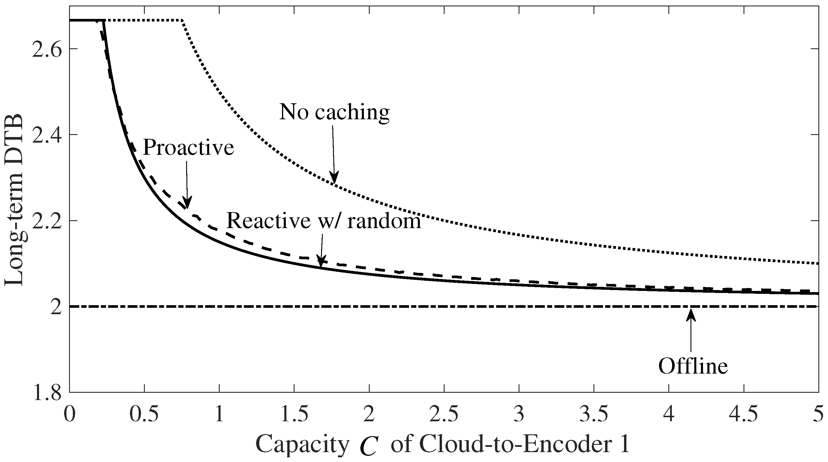
In this section, we evaluate the performance of the proposed online caching schemes numerically. We specifically consider the long-term DTB achievable by the proposed proactive scheme (34) and the proposed reactive scheme (35). For the latter, we evaluate the expectation in (36) via Monte Carlo simulations by averaging over a large number of realizations, i.e., 10,000, of the random process . It is assumed that the small-cell cache is empty at the start of simulation, i.e., at time .
The impact of the cloud-to-Encoder 1 capacity C is first considered in Figure 5. As a reference, we also plot the minimum DTB for offline caching in (23) and (24) and the performance with no caching, that is, in (24). For reactive caching, we assume random eviction for reactive caching. Parameters are set as , , and . It is seen that both proactive and reactive caching can significantly improve over the no caching scheme by updating the content stored at the small-cell BS. However, as the capacity of Cloud-to-Encoder 1 link decreases, it is deleterious in terms of delivery latency to use the link in order to update the cache content. As a result, if C is small enough, the performance of reactive and proactive caching coincides with the no caching system. When C is large enough, instead, the latency of cache update is negligible and both proactive and reactive schemes achieve the same DTB, which tends to the minimum offline DTB.
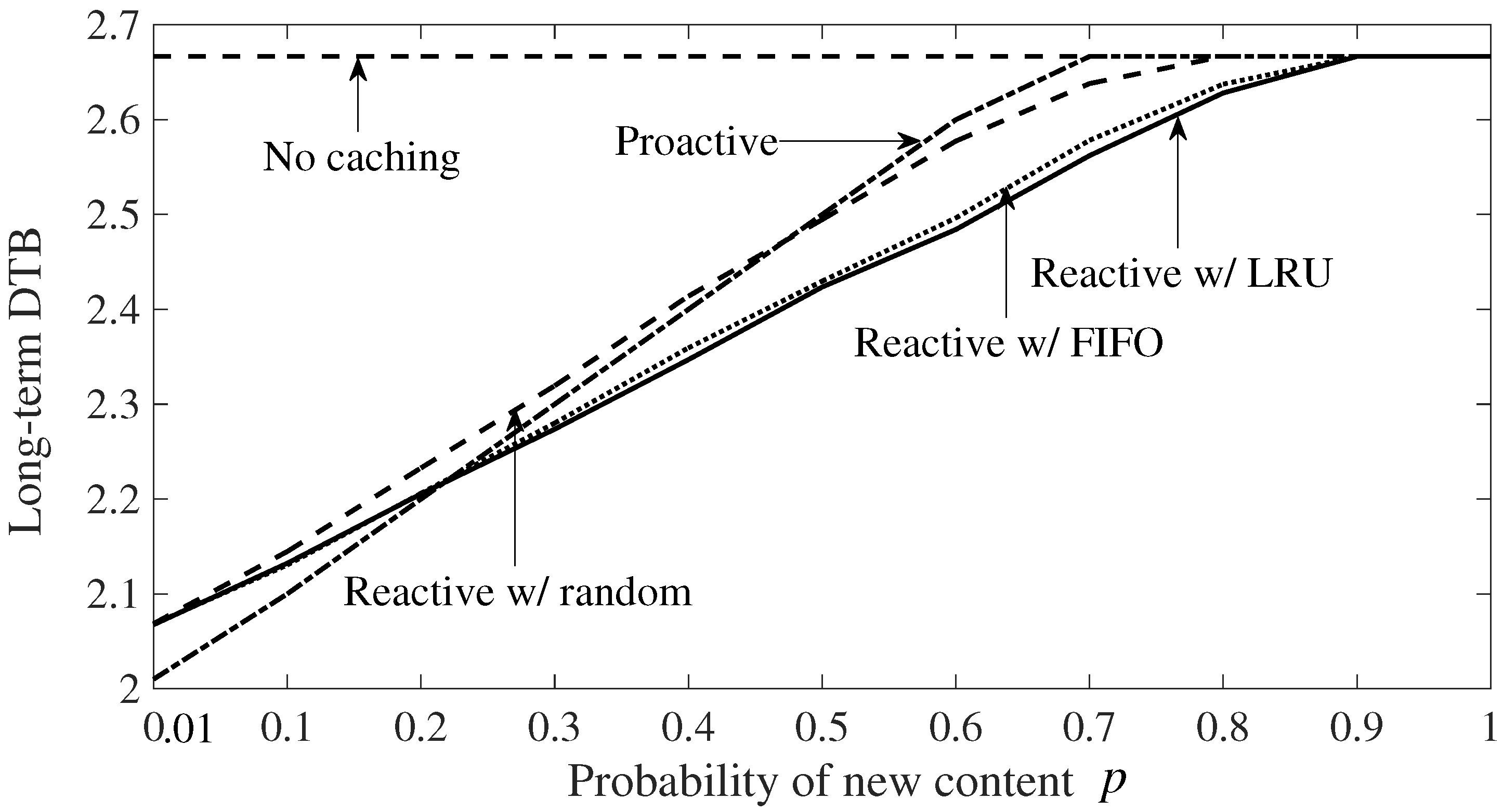
Next, we compare the performance of reactive and proactive online caching schemes as a function of the probability p of new content. As shown in Figure 6 for , , and , when p is small, proactive caching outperforms reactive caching, since it uses the Cloud-to-Encoder 1 connection only with rare event that there is a new popular file. On the other hand, when p is large, as explained in the previous section, the reactive approach yields a smaller latency than the proactive scheme. It is also seen that the LRU eviction strategy, whereby the replaced file is the one that has been least recently requested by any user, and FIFO eviction strategy, whereby the file that has been in the caches for the longest time is replaced, are both able to improve over randomized eviction.
7. Conclusions
Motivated by recent advances in cache and cloud-aided wireless network architectures, we have considered a fog-assisted system for content delivery. The system model includes a macro-BS that coexists with a cache and cloud-aided small-cell BS whose user can also be served by the macro-BS. Using the minimum delivery latency as performance measure, the trade-off between latency and system resources has been studied. A characterization of this optimal trade-off has been derived under a binary fading interference channel and in the presence of full CSI when the set of popular contents is fixed. For the alternative online scenario with time-varying set of popular files, the average DTB within a long time horizon is shown to be at most two times larger than for the offline scenario case when the capacity of the link used to update the cache content is small and to have otherwise a gap inversely proportional to this capacity.
Author Contributions
Osvaldo Simeone and Ravi Tandon conceived the system model and some of the key ideas behind achievability and converse; Seyyed Mohammadreza Azimi performed the analysis, carried out the numerical experiments, and wrote the paper with comments from Osvaldo Simeone and Ravi Tandon. All authors have read and approved the final manuscript.
Conflicts of Interest
The authors declare no conflict of interest.
Appendix A. Proof of Converse for Proposition 1
Consider any request vector containing two arbitrary, different files and , and any coding scheme satisfying as . The following set of inequalities is based on the fact that, under any such coding scheme, a hypothetical decoder provided with the CSI vector , with the cached contents and in (2) relative to files and , and with the signal , to be described below, must be able to decode both messages and . The signal is such that if and otherwise. Note, therefore, that as long as either or both and are equal to one. The intuition here is that from and , the hypothetical decoder can recover and hence ; while from , and , the decoder can reconstruct and hence decode . Details are as follows
where indicates any function that satisfies as . In above derivation, (a) follows from the facts that: (i) is a function of , , , and , since can be assumed to depend on without loss of generality only on and , and the vector can be obtained from and ; (ii) is a function of ; (b) follows from Fano’s inequality; (c) follows from the fact that the messages are independent of channel realization and from Fano inequality ; (d) hinges on the cache constraint (3) and by the following bounds
where is the set of all channel states and the last inequality follows from the fact that the entropy in all states is maximized for Bernoulli. For , (A1) yields the bound on the minimum DTB
Based on the fact that requested files should be retrieved from the received signals, another bound can be derived as follows:
where (a) follows from Fano’s inequality; (b) follows from the fact that channel gains are independent from files; (c) follows in a manner similar to (A2); and (d) is due to the fact that the entropy terms in the previous step are maximized by choosing and to be independent and identically distributed as Bernoulli. With , we obtain the bound
Appendix B. Proof of Converse for Proposition 2
Let us denote the normalized latency on the Cloud-to-Encoder 1 link and the normalized latency on the channel between encoders and decoders. We first observe that, following the same argument as in (A4)–(A7), we have the bound
for any sequence of feasible policies. We now obtain a lower bound on both normalized delays and by observing that a hypothetical decoder provided with the CSI vector , with the cached content and in (2), with the cloud-aided message , and with the signal described in Appendix A can decode both messages and . Details are as follows
where, as in Appendix A, indicates any function that satisfies as . In above derivation, steps (a)–(b) follow as steps (a)–(b) in (A1), where we note that the inequality by Fano inequality, while (c) hinges on the cache constraint (3) and the bound due to the capacity constraint on the Cloud-to-Encoder 1 link. As , the inequality (A9) yields the bound on the latency components and
- For , the bound (A10), directly yields
Appendix C. Proof of Proposition 5
To obtain a lower bound on the long-term DTB, following [16], we consider an enhanced system in which, at each time slot t, the small-cell BS is informed of the optimal cache content of an offline scheme tailored to the current popular set . In this system, at each time slot t, with probability of p there is a new file in the set of popular files, and hence the probability that an uncached file is requested by one of the users is . As a result, the DTB in time slot t for the genie-aided system can be lower bounded as
where is the minimum DTB for the offline caching set-up in Proposition 2, while is a lower bound on the minimum DTB for offline caching in which all files but one can be cached.
To obtain the lower bound , we start by noting that the set-up is equivalent to that for the proof in Appendix B with the only difference is that one of the requested files by users cannot be cached at the small-cell BS. Since the probability of error (31) should be small for any request vector, in order to obtain a lower bound, we assume that the message requested by user 1 cannot be cached at the small-cell BS. Using the resulting condition in step (b) of (50) yields the inequality
and hence, letting as , we have the inequality
- For , the bound (A14), directly yields
Appendix D. Proof of Proposition 6
The lower bound follows directly from Proposition 5. To prove the upper bound, we leverage the following lemma.
Lemma A1.
For any , we have the following inequality
Proof.
See Appendix E. ☐
Using Proposition 4 and Lemma A1, an upper bound on the long-term DTB of the proposed reactive caching scheme is obtained as
where
Since the additive gap (A20) is a decreasing function of N and an increasing function of p and , it can be further upper bounded by setting , and . By plugging , we have
The upper bound in (A21) is obtained using the fact that the maximum delivery latency namely, is achieved when both requested files are delivered by transmission from macro-BS. To complete the proof, we consider the following regimes
- Low capacity regime (): In this regime, using Propositions 2 and 5, the lower bound isTo prove the upper bound, we consider the following two sub-regimes
- −
- Low cache regime (): In this case, using Proposition 2 and (A21), we haveUsing Proposition 2, the minimum offline DTB is and therefore we havewhere follows from and follows from .
- −
Appendix E. Proof for Lemma A1
To prove Lemma A1, for any given , we first define
where given by (14). Then, we consider separately small-cache regime with , medium-cache regime and the high-cache regime with .
- Medium-cache Regime (): Using (24), we have the following upper boundwhere is obtained by omitting the negative terms.
References
- Shanmugam, K.; Golrezaei, N.; Dimakis, A.G.; Molisch, A.F.; Caire, G. Femtocaching: Wireless content delivery through distributed caching helpers. IEEE Trans. Inf. Theory 2013, 59, 8402–8413. [Google Scholar] [CrossRef]
- Bastug, E.; Bennis, M.; Debbah, M. Living on the edge: The role of proactive caching in 5G wireless networks. IEEE Commun. Mag. 2014, 52, 82–89. [Google Scholar] [CrossRef] [Green Version]
- Maddah-Ali, M.A.; Niesen, U. Cache Aided Interference Channels. 2015. Available online: http://arxiv.org/abs/1510.06121 (accessed on 21 October 2015).
- Maddah-Ali, M.A.; Niesen, U. Cache aided interference channels. In Proceedings of the 2015 IEEE International Symposium on Information Theory (ISIT), Hong Kong, China, 7–12 July 2015; pp. 809–813. [Google Scholar]
- Sengupta, A.; Tandon, R.; Simeone, O. Cache-aided wireless networks: Tradeoffs between storage and latency. In Proceedings of the Annual Conference on Information Science and Systems (CISS), Princeton, NJ, USA, 16–18 March 2016; pp. 320–325. [Google Scholar]
- Naderializadeh, N.; Maddah-Ali, M.A.; Avestimehr, A.S. Fundamental limits of cache-aided interference management. IEEE Trans. Inf. Theory 2017, 63, 3092–3107. [Google Scholar] [CrossRef]
- Xu, F.; Liu, K.; Tao, M. Cooperative Tx/Rx caching in interference channels: A storage-latency tradeoff study. In Proceedings of the 2016 IEEE International Symposium on Information Theory (ISIT), Barcelona, Spain, 7–12 July 2016; pp. 2034–2038. [Google Scholar]
- Roig, J.S.P.; Gunduz, D.; Tosato, F. Interference Networks with Caches at Both Ends. 2017. Available online: http://arxiv.org/abs/1703.04349 (accessed on 13 March 2017).
- Naderializadeh, N.; Maddah-Ali, M.A.; Niesen, U. On the Optimality of Separation between Caching and Delivery in General Cache Networks. In Proceedings of the 2017 IEEE International Symposium on Information Theory (ISIT), Aachen, Germany, 25–30 June 2017; pp. 1–5. [Google Scholar]
- Cao, Y.; Tao, M.; Xu, F.; Liu, K. Fundamental Storage-Latency Tradeoff in Cache-Aided MIMO Interference Networks. Available online: http://arxiv.org/abs/1609.01826 (accessed on 7 September 2016).
- Tandon, R.; Simeone, O. Cloud aided wireless networks with edge caching: Fundamental latency trade offs in Fog radio access networks. In Proceedings of the 2016 IEEE International Symposium on Information Theory (ISIT), Barcelona, Spain, 7–12 July 2016; pp. 2029–2033. [Google Scholar]
- Sengupta, A.; Tandon, R.; Simeone, O. Fog-Aided Wireless Networks for Content Delivery: Fundamental Latency Trade-Offs. 2016. Available online: http://arxiv.org/abs/1605.01690 (accessed on 5 May 2016).
- Koh, J.; Simeone, O.; Tandon, R.; Kang, J. Cloud-aided edge caching with wireless multicast fronthauling in fog radio access networks. In Proceedings of the IEEE Wireless Communications and Networking Conference (WCNC), San Francisco, CA, USA, 19–22 March 2017; pp. 1–6. [Google Scholar]
- Girgis, M.; Ercetiny, O.; Nafie, M.; ElBatt, T. Decentralized coded caching in wireless networks: Trade-off between storage and latency. In Proceedings of the 2017 IEEE International Symposium on Information Theory (ISIT), Aachen, Germany, 25–30 June 2017; pp. 1–5. [Google Scholar]
- Goseling, J.; Simeone, O.; Popovski, P. Delivery Latency Regions in Fog-RANs with Edge Caching and Cloud Processing. 2017. Available online: http://arxiv.org/abs/1701.06303 (accessed on 23 January 2017).
- Azimi, S.M.; Simeone, O.; Tandon, R. Online Edge Caching in Fog-Aided Wireless Network. 2017. Available online: http://arxiv.org/abs/1701.06188 (accessed on 22 January 2017).
- Azimi, S.M.; Simeone, O.; Tandon, R. Fundamental limits on latency in small-cell caching systems: An information-theoretic analysis. In Proceedings of the IEEE Global Communication Conference (GLOBECOM), Washington, DC, USA, 4–8 December 2016; pp. 1–6. [Google Scholar]
- Kakar, J.; Gherekhloo, S.; Sezgin, A. Fundamental Limits on Delivery Time in Cloud- and Cache-Aided Heterogeneous Networks. 2017. Available online: http://arxiv.org/abs/1706.07627 (accessed on 23 June 2017).
- Peng, X.; Shen, J.C.; Zhang, J.; Kang, J.; Letaief, K.B. Joint data assignment and beamforming for backhaul limited caching networks. In Proceedings of the IEEE International Symposium on Personal, Indoor and Mobile Radio Communications (PIMRC), Washington, DC, USA, 2–5 September 2014; pp. 1370–1374. [Google Scholar]
- Park, S.-H.; Simeone, O.; Shamai, S. Joint optimization of cloud and edge processing for Fog radio access networks. IEEE Trans. Wirel. Commun. 2016, 15, 7621–7632. [Google Scholar] [CrossRef]
- Tao, M.; Chen, E.; Zhou, H.; Yu, W. Content-Centric Sparse Multicast Beamforming for Cache-Enabled Cloud RAN. IEEE Trans. Wirel. Commun. 2016, 15, 6118–6131. [Google Scholar] [CrossRef]
- Azari, B.; Simeone, O.; Spagnolini, U.; Tulino, A.M. Hypergraph-based analysis of clustered cooperative beamforming with application to edge caching. IEEE Wirel. Commun. Lett. 2016, 5, 84–87. [Google Scholar] [CrossRef]
- Park, S.H.; Simeone, O.; Shamai, S. Joint cloud and edge processing for latency minimization in fog radio access networks. In Proceedings of the IEEE International Workshop on Signal Processing Advances in Wireless Communications (SPAWC), Edinburgh, UK, 3–6 July 2016; pp. 1–5. [Google Scholar]
- Martina, V.; Garetto, M.; Leonardi, E. A unified approach to the performance analysis of caching systems. In Proceedings of the IEEE Conference on Computer Communications (INFOCOM), Toronto, CA, Canada, 27 May–2 April 2014; pp. 2040–2048. [Google Scholar]
- Zhu, Y.; Guo, D. Ergodic fading Z-interference channels without state information at transmitters. IEEE Trans. Inf. Theory 2011, 57, 2627–2647. [Google Scholar] [CrossRef]
- Vahid, A.; Maddah-Ali, A.S.; Avestimehr, A.S. Capacity results for binary fading interference channels with delayed CSIT. IEEE Trans. Inf. Theory 2014, 60, 6093–6130. [Google Scholar] [CrossRef]
- Avestimehr, A.S.; Diggavi, S.N.; Tse, D.N.C. Wireless Network Information Flow: A Deterministic Approach. IEEE Trans. Inf. Theory 2011, 57, 1872–1905. [Google Scholar] [CrossRef]
- Tse, D.N.C.; Yates, R.D. Fading Broadcast Channels With State Information at the Receivers. IEEE Trans. Inf. Theory 2012, 58, 3453–3471. [Google Scholar] [CrossRef]
- Pedarsani, R.; Maddah-Ali, M.A.; Niesen, U. Online coded caching. IEEE Trans. Inf. Theory 2016, 24, 836–845. [Google Scholar] [CrossRef]
Figure 1.
Cloud and edge-aided data delivery over binary fading interference channels.
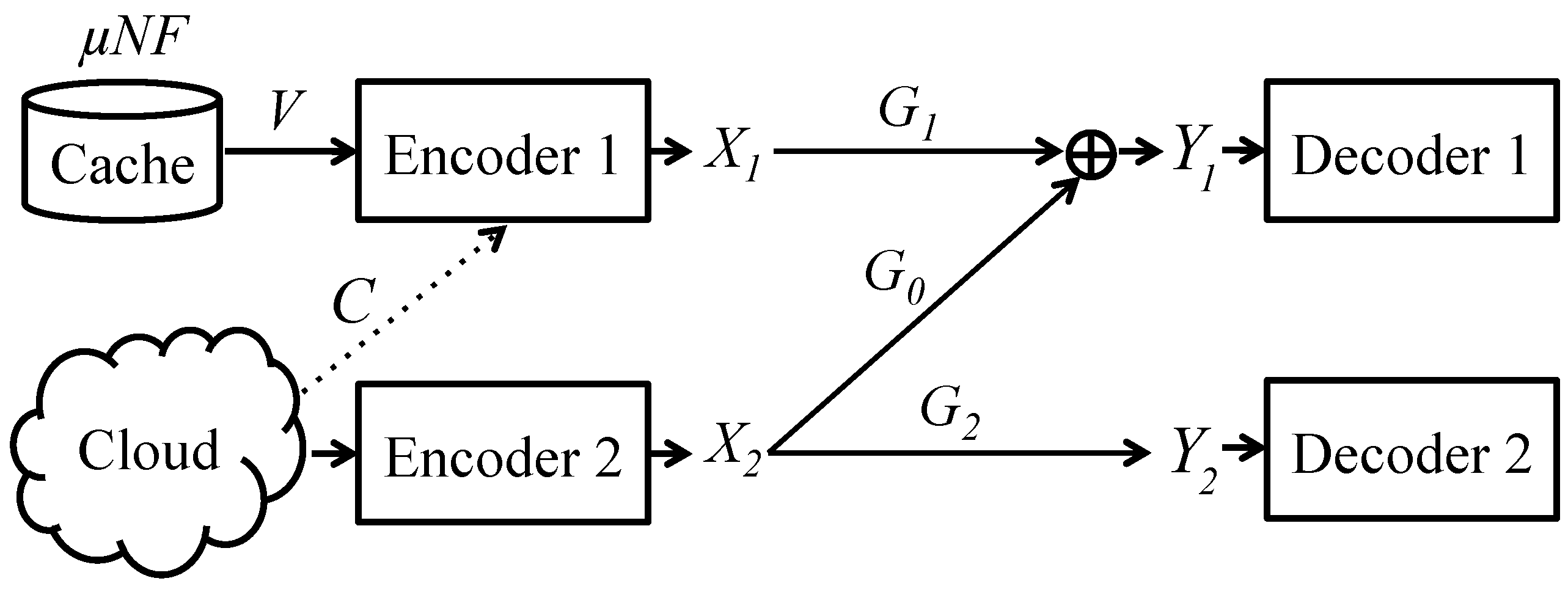
Figure 2.
Optimum fractional cache size as a function of for different values of , which ranges from 0 to 1 with step size .
Figure 2.
Optimum fractional cache size as a function of for different values of , which ranges from 0 to 1 with step size .
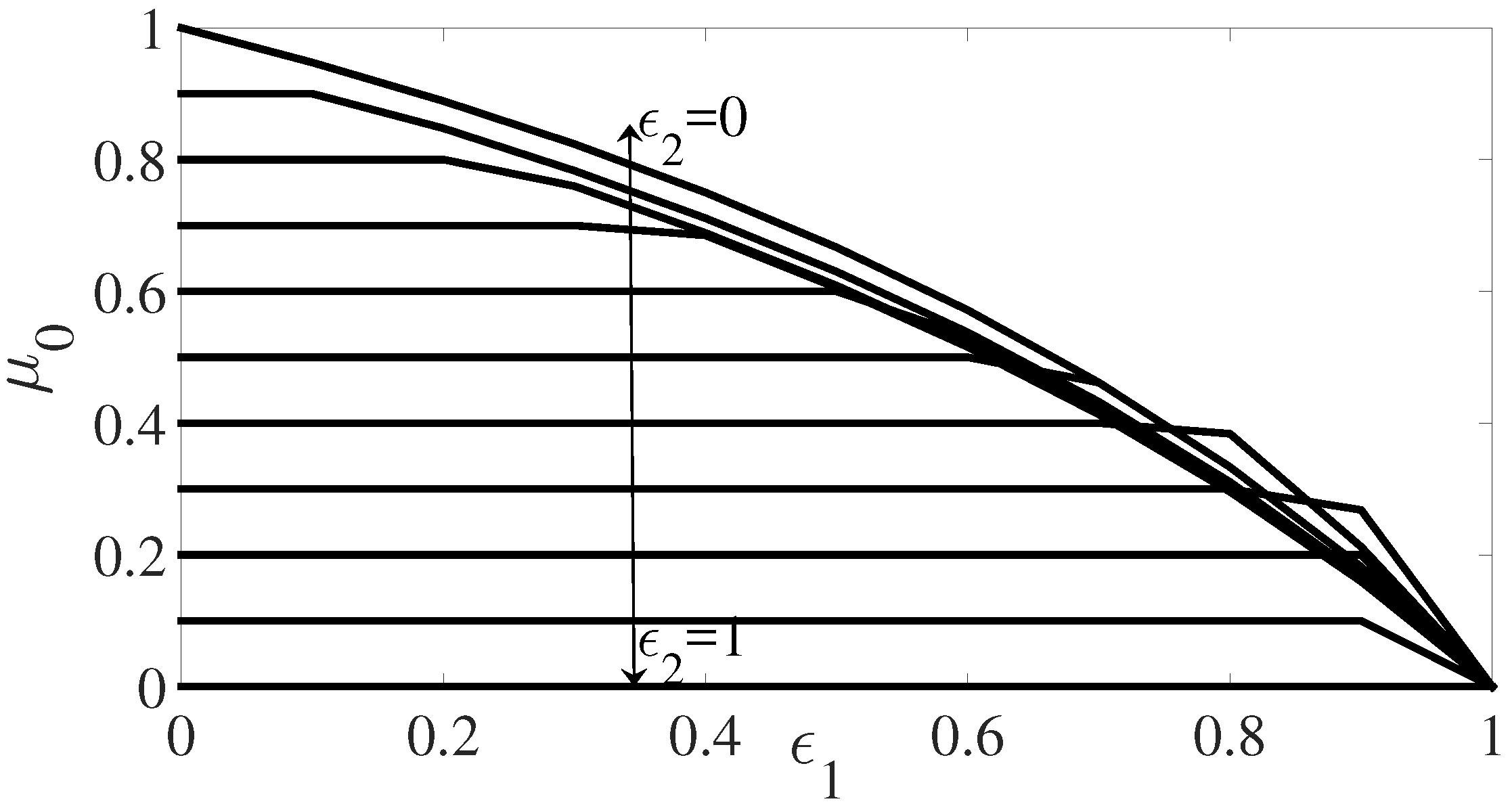
Figure 3.
Minimum Delivery Time per Bit (DTB) for the system in Figure 1 with .
Figure 3.
Minimum Delivery Time per Bit (DTB) for the system in Figure 1 with .
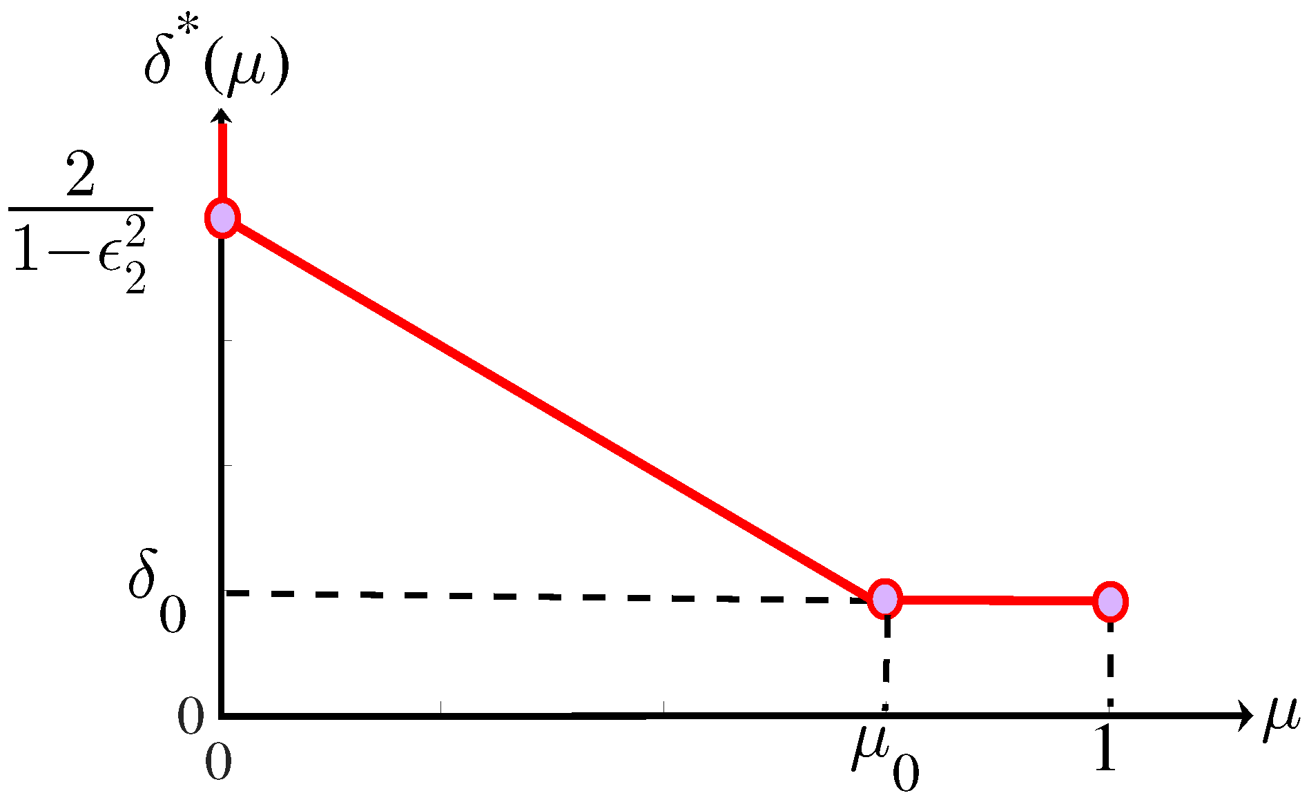
Figure 4.
Minimum Delivery Time per Bit (DTB) for the system in Figure 1.
Figure 4.
Minimum Delivery Time per Bit (DTB) for the system in Figure 1.
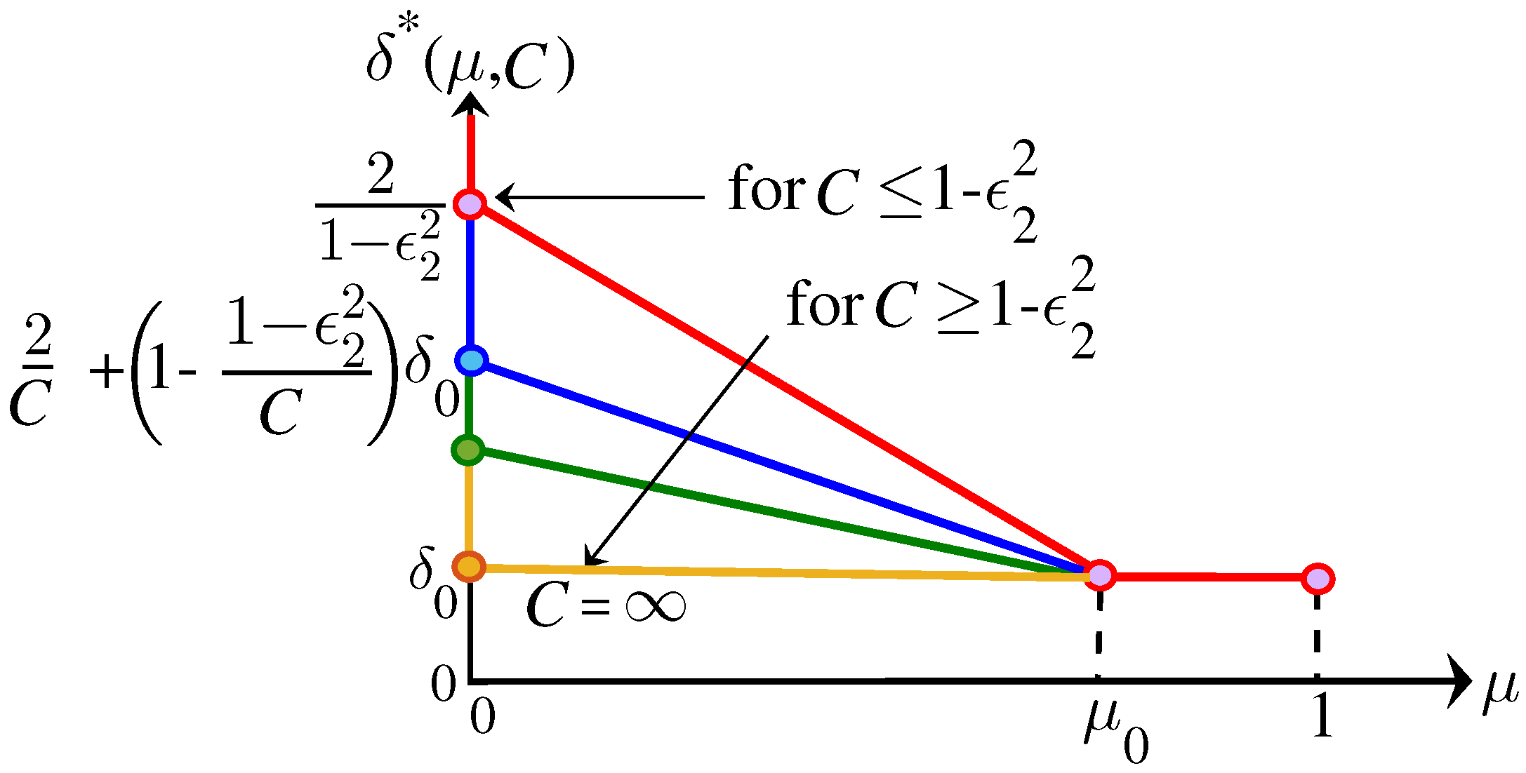
Figure 5.
Achievable long-term DTB versus the capacity C of the Cloud-to-Encoder 1 for proactive scheme (34) and reactive caching with random eviction (35). For reference, the DTB with no caching, namely , and the offline minimum DTB (23) and (24) are also shown (, , , ).


© 2017 by the authors. Licensee MDPI, Basel, Switzerland. This article is an open access article distributed under the terms and conditions of the Creative Commons Attribution (CC BY) license (http://creativecommons.org/licenses/by/4.0/).
Share and Cite
MDPI and ACS Style
Azimi, S.M.; Simeone, O.; Tandon, R. Content Delivery in Fog-Aided Small-Cell Systems with Offline and Online Caching: An Information—Theoretic Analysis. Entropy 2017, 19, 366. https://doi.org/10.3390/e19070366
AMA Style
Azimi SM, Simeone O, Tandon R. Content Delivery in Fog-Aided Small-Cell Systems with Offline and Online Caching: An Information—Theoretic Analysis. Entropy. 2017; 19(7):366. https://doi.org/10.3390/e19070366
Chicago/Turabian StyleAzimi, Seyyed Mohammadreza, Osvaldo Simeone, and Ravi Tandon. 2017. "Content Delivery in Fog-Aided Small-Cell Systems with Offline and Online Caching: An Information—Theoretic Analysis" Entropy 19, no. 7: 366. https://doi.org/10.3390/e19070366
Note that from the first issue of 2016, this journal uses article numbers instead of page numbers. See further details here.