Entropic Phase Maps in Discrete Quantum Gravity

Department of Mathematics, William Carey University, 710 William Carey Parkway, Hattiesburg, MS 39401, USA
Entropy 2017, 19(7), 322; https://doi.org/10.3390/e19070322
Submission received: 26 May 2017
/
Revised: 20 June 2017
/
Accepted: 25 June 2017
/
Published: 30 June 2017
(This article belongs to the Special Issue Quantum Information and Foundations)
Abstract
:Path summation offers a flexible general approach to quantum theory, including quantum gravity. In the latter setting, summation is performed over a space of evolutionary pathways in a history configuration space. Discrete causal histories called acyclic directed sets offer certain advantages over similar models appearing in the literature, such as causal sets. Path summation defined in terms of these histories enables derivation of discrete Schrödinger-type equations describing quantum spacetime dynamics for any suitable choice of algebraic quantities associated with each evolutionary pathway. These quantities, called phases, collectively define a phase map from the space of evolutionary pathways to a target object, such as the unit circle , or an analogue such as or . This paper explores the problem of identifying suitable phase maps for discrete quantum gravity, focusing on a class of -valued maps defined in terms of “structural increments” of histories, called terminal states. Invariants such as state automorphism groups determine multiplicities of states, and induce families of natural entropy functions. A phase map defined in terms of such a function is called an entropic phase map. The associated dynamical law may be viewed as an abstract combination of Schrödinger’s equation and the second law of thermodynamics.
1. Introduction
1.1. Path Summation in Quantum Gravity
Feynman’s path summation approach to quantum theory [1], originally developed in the non-relativistic context of four-dimensional Euclidean spacetime , has since been abstracted and generalized to apply to a wide variety of situations in which quantum effects play a significant role, including the study of fundamental spacetime structure and quantum gravity. In the latter setting, the objects over which summation is performed are no longer spaces of paths in low-dimensional real manifolds whose elements represent events, but spaces of evolutionary pathways in configuration spaces whose elements represent histories, i.e., entire spacetimes. The distinction between summing over evolutionary pathways for histories and summing over histories themselves becomes significant in the background independent context, where each pathway represents a history together with a generalized frame of reference, and where different pathways may encode identical physics. For both conceptual and computational reasons, histories incorporating a version of discreteness and a notion of causal structure are especially attractive for studying quantum gravity. Such histories include “purely causal” objects such as causal sets [2] and causal networks [3,4,5], “mostly causal” objects such as causal dynamical triangulations [6] and quantum causal histories [7], and objects incorporating a significant degree of additional structure, such as spin foams [8,9], quantum cellular automata [10], causal fermion systems [11,12], and tensor networks [13]. The histories studied in this paper, called acyclic directed sets, resemble causal sets and causal networks, but with a few important distinctions [14,15,16].
1.2. Path Summation Rudiments
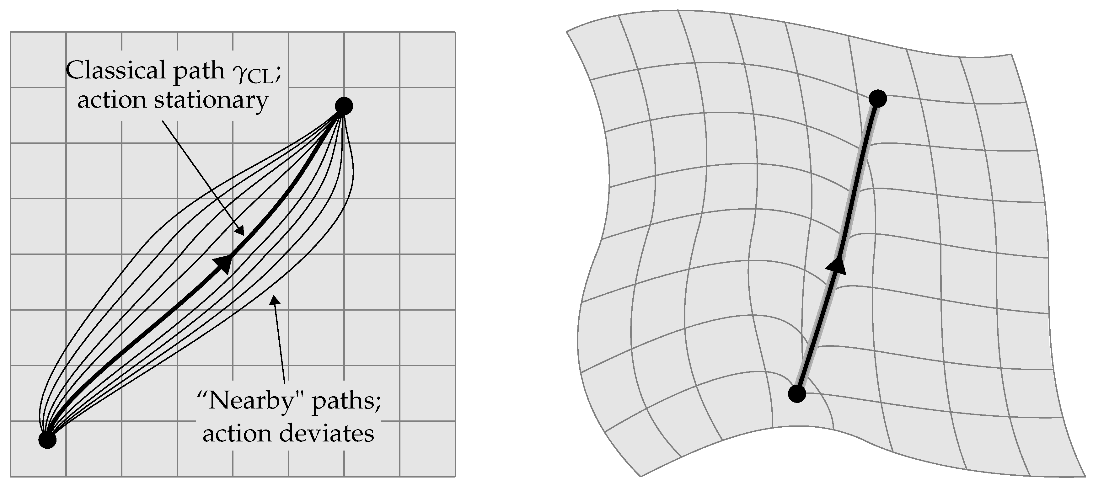
I recall here a few basic notions regarding conventional path summation. In ordinary quantum mechanics and quantum field theory, one considers directed paths representing possible particle trajectories in a fixed spacetime manifold, such as Euclidean spacetime or Minkowski spacetime . Such paths are illustrated in the left-hand diagram in Figure 1, adapted from Figure 6.2.2 of [14]. One begins with a classical theory, whose dynamics is determined by a Lagrangian encoding information about motion-related or metric quantities. may be regarded as an infinitesimal path functional, i.e., a function of the particle motion whose value depends only on instantaneous information along . This viewpoint generalizes naturally to more abstract settings. The classical action is given by integrating along with respect to time. Hamilton’s principle states that the classical path renders the classical action stationary. Heuristically, this means that “chooses” from among other alternatives by how varies with . The classical equations of motion are the Euler–Lagrange equations for , derived via Hamilton’s principle.
In the corresponding quantum theory, the behavior of the particle depends on contributions from every possible path. To quantify this dependence, one defines a phase map on a space of paths in spacetime, given by Feynman’s formula
where and ħ is Planck’s reduced constant. For convenience, I use the term “phase” for the value itself, rather than for the “angle” in the complex exponential. One then performs a path integral to “sum together” these phases. Feynman’s path integral for paths in a subset R of is the prototypical example. Its value is interpreted as a complex quantum amplitude for R, encoding the probability that the particle follows a path through R. Due to Hamilton’s principle, phases for paths near the classical path combine via constructive interference to yield relatively large amplitudes for neighborhoods of , while phases for faraway paths destructively interfere. Schrödinger’s equation for ordinary nonrelativistic quantum theory
may be derived from Feynman’s path integral [1]. Here, is the state function for the particle, and is the Hamiltonian operator.
1.3. Effects of Gravity
Gravitation alters this picture by introducing interaction between spacetime and its material content. It no longer suffices to consider particle paths in a fixed spacetime manifold, because different paths induce different local responses in spacetime geometry. The right-hand diagram in Figure 1 illustrates this complication, showing a region of spacetime “warping” around a path. Absence of a fixed spacetime background in this context is called background independence. Einstein’s equation, conventionally expressed in the form
quantifies this coupling between geometry and matter under the framework of general relativity. Here, is the Ricci curvature tensor, R is the scalar curvature, is the metric tensor, is the cosmological constant, G is Newton’s gravitational constant, c is the speed of light, and is the stress-energy tensor. Ultimately, one expects both geometry and matter to emerge from some deeper structural substratum, and this has been a consistent theme of fundamental physics since the early unification efforts of Einstein, Kaluza and Klein, Weyl, and a few others. Unification would offer a perfect version of background independence by eliminating all distinction between a background “arena” and foreground “objects”. Discrete causal theory [14] represents one specific effort toward the goal of unification. More generally, any background independent adaptation of path summation associates a different copy of spacetime with each possible distribution of matter and energy, and this leads to sums involving entire configuration spaces of spacetimes. Each such spacetime is classically self-contained, in the sense that it describes its own complete version of events, and has no ordinary causal interaction with other possible spacetimes. In this context, a spacetime is often called a history, and a configuration space of spacetimes is called a history configuration space.
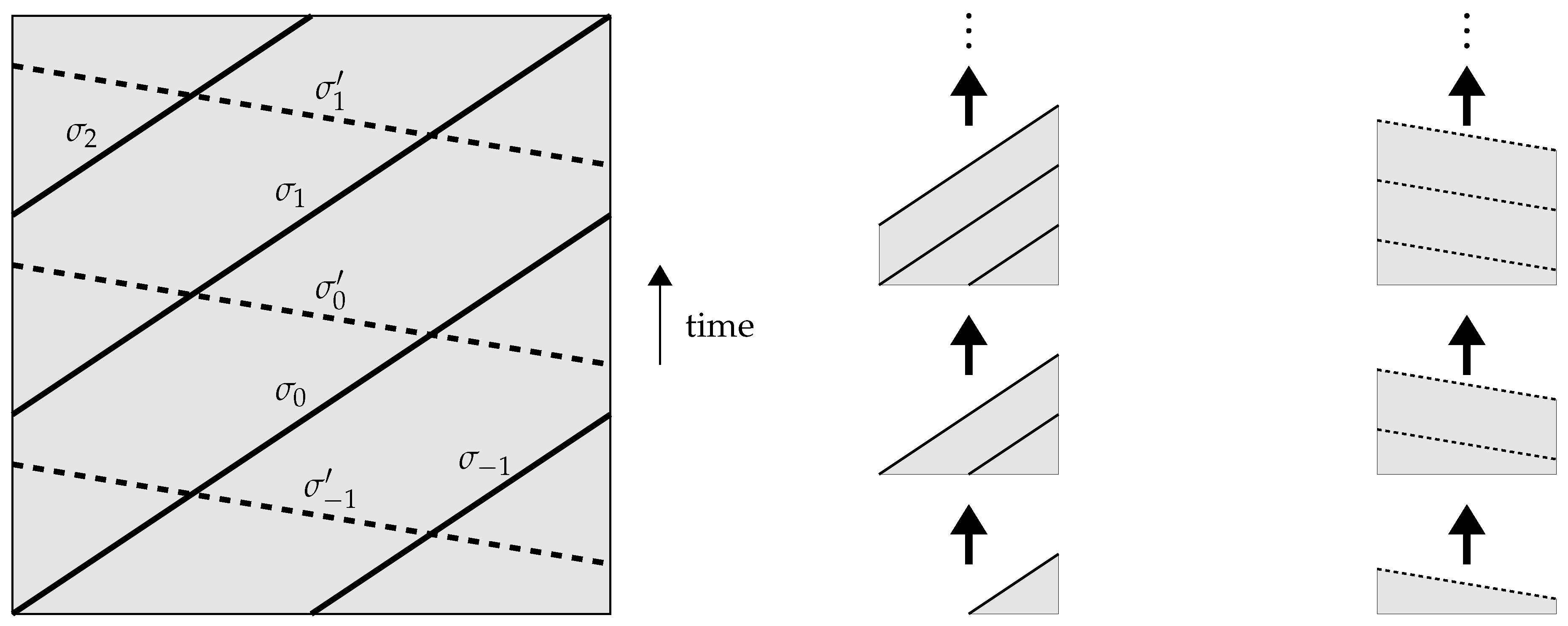
A subset of a history configuration space equipped with a total order, such as the image of a non-self-intersecting directed path in , does not represent “classical dynamics”, since each history contains its own complete description of events. However, certain special totally ordered subsets of may be interpreted as representing “growth” or “development” of one history into another, and such subsets are called evolutionary pathways in . Technical requirements for evolutionary pathways are discussed below. Such pathways may or may not possess initial or terminal histories, depending on the structure of . However, any pair of pathways in sharing a common terminal history, or a common “limit” in more general settings, describe identical physics from different points of view. A familiar example is given by partitioning Minkowski spacetime via two different integer-indexed families and of spacelike sections, as illustrated in the left-hand diagram in Figure 2. This diagram follows the usual convention of suppressing two spacelike dimensions, with time running vertically up the page. Edges do not represent physical boundaries, but merely delimit the finite region shown. Discrete evolutionary pathways for may be defined via these partitions, as shown in the middle and right-hand diagrams. One may completely foliate by similar families, thereby defining continuous pathways in a configuration space of Lorentzian manifolds. However, the simpler discrete picture shown here, in which is partitioned into increments of nontrivial causal extent, is more illustrative of the discrete processes studied in this paper.
Both evolutionary pathways illustrated in Figure 2 describe the same empty, flat spacetime represented by . However, they offer different perspectives regarding the evolution of this spacetime. These may be identified with different inertial frames of reference on , since and are families of parallel spacelike hyperplanes. In more abstract settings, histories may not encode recognizable geometry, so the relativistic idea of frames of reference must be generalized. However, the conceptual content remains unchanged: each evolutionary pathway in a history configuration space describes a history together with a generalized frame of reference for this history. To qualify as an evolutionary pathway, a totally ordered subset of must satisfy the property that “later histories in are evolutionary descendants of earlier histories”. Mathematically, this means that the total order on must be derived naturally from the structure of . The most convenient case is when itself possesses natural order-theoretic structure from which evolutionary relationships may be deduced in a self-evident way. This is the case for discrete causal theory.
1.4. Motivation for Entropic Phase Maps
Histories modeled by objects called countable star finite acyclic directed sets induce discrete causal history configuration spaces called kinematic schemes, with properties superior in some ways to those of similar spaces arising in causal set theory, causal dynamical triangulations, and related approaches. These objects are formally defined in Section 2. Path summation over a kinematic scheme , together with other natural machinery, enables derivation of discrete causal Schrödinger-type equations such as Equation (1.1.2) of [14]. This equation is reproduced here as Equation (4):
The meaning of this equation is explained in Section 2, and more thoroughly in [14], but I briefly describe its content here. The function is a generalized state function, called the past state function, while R is a set of relations representing natural relationships between pairs of histories in , called co-relative histories. Sequences of co-relative histories fit together to define evolutionary pathways in , called co-relative kinematics. The relations r and are elements of R representing specific co-relative histories. The precursor symbol ≺ in the expression indicates that the evolutionary relationship represented by r is a possible sequel to the evolutionary relationship represented by .
Remaining to be identified in Equation (4) is the relation function , which is the entity of principal interest in this paper. This function assigns to each element r of R a phase belonging to some target object T. The most obvious choice for T is the unit circle , viewed as a subobject of the complex field , and this is the target object focused on here. However, other choices may be studied in more general contexts. For reasons explained in [14], the unit spheres and , viewed as subobjects of the quaternions and octonions , respectively, are potentially interesting alternatives. At a finer level of detail, it may be appropriate to consider discrete subobjects of , , or , which possess interesting algebraic properties. Alternatively, T might be an object at a higher level of algebraic hierarchy, such as a monoidal category. In any case, T must possess a “multiplicative” operation, enabling the factor to multiply the sum in Equation (4). Extending via this operation, as described below, defines a phase map on the space of co-relative kinematics in . The form of Equation (4) assumes that generates in this way; otherwise, the equation must be generalized. Under this assumption, provides specific dynamical content to the equation, and thereby defines a quantum dynamical law governing fundamental spacetime structure.
The elements of the relation set R in Equation (4) encode information up to first order at the quantum level, in the sense that they represent individual stages of evolution in . Hence, is analogous to an infinitesimal path functional on , i.e., a generalized Lagrangian. Similarly, may be regarded as a generalized action. However, to simplify the form of Equation (4), the appropriate analogue of the exponentiation appearing in Feynman’s phase map (1) is “built in” to the definition of . Hence, the quantities I call “phases” throughout the remainder of the paper are analogous to Feynman’s complex exponentials themselves, not to the corresponding “angles” . The phase of a co-relative kinematics is therefore a product of phases of individual relations r along , rather than a sum or integral. More precisely, one may define a concatenation product ⊔ joining co-relative kinematics “end-to-end”, under which may be factored into a product of individual relations Extending multiplicatively then means that , where the product is in the target object T. Questions of convergence are important in general, but are not examined here, since one may go quite far under finiteness assumptions.
This paper explores the problem of identifying suitable phase maps for discrete quantum gravity, focusing on a class of -valued maps defined in terms of terminal states of histories D along evolutionary pathways in a history configuration space . Here, is a kinematic scheme of star finite acyclic directed sets D, is a co-relative kinematics, and encodes “recent” causes and effects in D. Invariants such as state automorphism groups determine multiplicities of states, and induce natural families of entropy functions. Resolution entropy is defined via a “coarse-graining” procedure called causal atomic resolution, analogous to conventional partitioning of state space into families of states sharing “macroscopic” properties. Superset entropy is defined by counting the number of ways in which a terminal state may embed into a larger state called a superset of . A large state automorphism group corresponds to a small number of such supersets, and therefore implies low entropy. Labeled entropy is defined by counting the number of ways to label elements of ; again, large implies low entropy. Symmetry entropy, by contrast, is defined by counting the elements of itself, so large implies high entropy in this context. A primitive version of symmetry entropy is discussed in Section 8.2 of [14]. A phase map defined in terms of such entropic quantities, or related quantities such as entropy per unit volume, is called an entropic phase map. The resulting version of Equation (4) may be viewed as an abstract combination of Schrödinger’s equation and the second law of thermodynamics, which arises entirely from the structure of .
Section 2 presents the necessary background from discrete causal theory [14] to support the development and description of these ideas. Section 2.1 briefly outlines the conceptual and philosophical foundations of discrete causal theory. Section 2.2 describes the classical version of the theory, expressed in terms of countable star finite acyclic directed sets. Section 2.3 sketches the theory of relation space, which addresses certain technical difficulties in earlier versions of the theory such as causal set theory. Section 2.4 describes the basics of discrete quantum causal theory. Section 3 examines entropy and the second law of thermodynamics in a broad context, introduces discrete causal analogues of familiar thermodynamic ideas such as state space, and develops the specific notions of entropy mentioned above. Section 3.1 discusses entropy in general terms under a broad framework called entropy systems. Section 3.2 describes associated versions of the second law. Section 3.3 introduces discrete causal state spaces. Section 3.4 defines resolution, superset, labeled, and symmetry entropies. Section 4 introduces entropic phase maps, and examines some of their properties. Section 4.1 describes some simple versions of these maps explicitly. Section 4.2 discusses the problem of obtaining suitable interference effects analogous to those induced for Feynman’s phase map by Hamilton’s principle. Section 4.3 discusses some possible objections to the idea of entropic phase maps, and briefly examines an alternative approach involving a more conventional notion of action. Section 4.4 offers concluding remarks, and mentions some mathematical problems whose solution would enhance the study of entropic phase maps.
2. Discrete Causal Theory
2.1. Causal Metric Hypothesis
Discrete causal theory is a general approach to fundamental physics that emphasizes discrete spacetime models equipped with directed structure encoding cause-and-effect relationships between pairs of events. Included under this umbrella are causal set theory [2], causal dynamical triangulations [6], and quantum causal histories [7]. Similar ideas contribute to loop quantum gravity [8,9], information-related approaches involving causal networks or cellular automata [10,17,18], causal fermion systems [11], and the theory of tensor networks [13]. The version of discrete causal theory used in this paper is distinct from all these, but may be regarded as an enhanced version of causal set theory [14]. Clean and appealing basic structure is an asset of discrete causal theory, but its principal motivation derives from technical results called metric recovery theorems, discussed in Section 2.2, which demonstrate that discrete causal models can reproduce relativistic spacetime geometry at ordinary scales. Such models also avoid generic divergence problems, and offer potential explanatory advantages by allowing “pre-geometric” notions such as spacetime dimension to emerge dynamically. The reason why these models cannot yet replace relativistic geometry root and branch is because relativity explains how geometry evolves via Einstein’s Equation (3), while discrete causal dynamics remains primitive. This paper offers a modest contribution toward rectifying this deficiency.
A radical interpretation of the aforementioned metric recovery results is the causal metric hypothesis [14,15,16], which states that the structural properties of the universe, particularly the metric structure of spacetime, emerge from causal structure at the fundamental scale. This general idea forms the philosophical basis for discrete causal theory, but may be accorded different weights in different versions of the theory. The strong interpretation of the causal metric hypothesis ascribes all of physics, including “nongravitational matter”, to causal structure. In the context of entropic phase maps, the strong interpretation extends the thermodynamic hypothesis regarding gravitation [19] to treat matter and energy in similar terms. Alternatively, one may choose to restrict attention to gravity, leaving aside unification. In this context, matter and energy may be modeled by attaching auxiliary algebraic structure to causal structure. In either case, quantum theory arises via generalized path summation in a manner much simpler and more natural than conventional attempts to quantize relativistic geometry. The directed structures of individual discrete causal histories combine to induce higher-level multidirected structures on their history configuration spaces, analogous to higher-level geometric structures of moduli spaces in algebraic geometry. This iteration of structure enables a natural version of summation over evolutionary pathways, which leads to quantum dynamics governed by discrete causal Schrödinger-type equations such as Equation (4).
2.2. Classical Theory
The mathematical objects used to model discrete causal histories in this paper are called countable star finite acyclic directed sets. Before defining them formally, I make two clarifying remarks. First, these objects are conventionally called “directed graphs” rather than “directed sets”, because the latter term has a more specific conventional meaning. However, graph-theoretic terminology is awkward here, and “directed set” ideally communicates the intended notion of a set D equipped with directions between distinguished pairs of elements x and y. Such a direction is called a relation between x and y, with initial element x and terminal element y, and is denoted by . The precursor symbol ≺ generalizes the familiar less than symbol < on a totally ordered set such as . The relation is represented graphically by a directed edge between nodes representing x and y. A family of such relations is called a binary relation on D, denoted collectively by the same symbol ≺. Mathematically, ≺ is a subset of the Cartesian product . Dual usage of the word “relation” and the symbol ≺ for individual relations and for the set ≺ of all such individual relations is a standard convenience. Second, the choice to focus on acyclic directed sets rules out discrete causal analogues of closed causal curves, but this is a simplifying assumption that may be relaxed. It does not imply the view that quantum gravity necessarily forbids such structure. Countability and/or star finiteness may also be relaxed, though in my opinion there is limited motivation for doing so.
The following definitions are adapted from Sections 3.6 and 3.7 of [14]:
Definition 1.
A directed set is a set D equipped with a binary relation ≺. A morphism from a directed set to a directed set is a set map such that whenever . The category of directed sets is the category whose objects are directed sets and whose morphisms are morphisms of directed sets. A subobject of a directed set is a directed set , where is a subset of D, and where is a subset of ≺ consisting of relations between pairs of elements of . The causal dual of a directed set is the directed set , where if and only if .
Definition 2.
A multidirected set consists of a set of elements M, a set of relations R, and initial and terminal element maps and . A morphism from a multidirected set to a multidirected set consists of a map of elements and a map of relations , such that and for each r in R. The category of multidirected sets is the category whose objects are multidirected sets and whose morphisms are morphisms of multidirected sets. A subobject of a multidirected set is a multidirected set , where and are subsets of M and R, respectively, and where and are the restrictions of i and t to . The causal dual of a multidirected set is the multidirected set .
Definition 3.
A chain in a multidirected set is a sequence of relations such that . The past of an element x of is the set of all elements w in M such that there exists a chain with and . The future of x is the set of all elements y in M such that there exists a chain with and . An antichain in is a subset σ of M with no chain connecting any pair of its elements, distinct or otherwise. The past relation set of an element x in M is the set of all relations r in R such that . The future relation set of x is the set of all relations r in R such that . The relation set of x is the union .
For both directed sets and multidirected sets, an isomorphism is an invertible morphism, and an automorphism is a self-isomorphism. Isomorphic sets are usually considered to be equivalent. It is often convenient to denote a directed set or multidirected set by just D or M, respectively, or to write or to indicate that a set D or M is equipped with such structure. Similarly, the causal dual of a directed set D may be denoted by , and the causal dual of a multidirected set M by . A directed set may be recognized as a multidirected set whose set of relations is the binary relation ≺, and whose initial and terminal element maps are defined by setting and . For multidirected sets, the notation remains useful to indicate the existence of a relation r such that and , even though no binary relation is involved. The necessity to study multidirected sets arises at the quantum level, via iteration of structure.
A well-motivated version of discrete classical causal theory is defined by the axioms in Definition 4, adapted from Definition 4.10.1 of [14]. Symbols and terms are further discussed below.
Definition 4.
Five axioms for discrete classical causal theory are the following:
- 1.
- Binary axiom: Classical spacetime may be modeled as a directed set , whose elements represent events, and whose relations represent causal relationships between pairs of events.
- 2.
- Generalized measure axiom: D is equipped with a set function μ from the power set of D to the extended real numbers , which assigns finite positive values to nonempty finite subsets of D, and infinite values to infinite subsets of D.
- 3.
- Countability: D is countable.
- 4.
- Star finiteness: For every element x of D, the star of x is finite.
- 5.
- Acyclicity: D possesses no cycles, i.e., sequences of relations with .
The binary axiom specifies both a mathematical structure and a physical interpretation of this structure. The generalized measure axiom imposes no mathematical conditions on the remaining axioms, so it is allowed a range of possible versions, each specified by a choice of . The most attractive choices are similar to the counting measure used in early versions of causal set theory, which assigns to each subset of D its number of elements in fundamental units. The function is unrelated to the family of measures for an entropy system, introduced in Section 3.1. Since the star of x is just , star finiteness is equivalent to finiteness of relation sets . The physical meaning of this condition is that every event has only a finite number of direct causes and effects. The reason for using rather than involves topological bookkeeping that plays no direct role in this paper. The meanings of countability and acyclicity are self-evident. The discreteness of D is encoded in the generalized measure axiom and the axiom of star finiteness.
Figure 3, adapted from Figure 3.6.5 of [14], illustrates different types of directed sets and multidirected sets. Elements are represented by nodes, and relations by directed edges. In the third and fourth diagrams, directions of relations are indicated by arrows, while in the first and second diagrams, directions are inferred via an “up the page” convention analogous to the convention for the direction of time in Minkowski spacetime diagrams. This convention applies only to acyclic directed sets. The first diagram illustrates a causal set, i.e., a countable, irreflexive, transitive, interval finite directed set . Irreflexivity means that C contains no “self-relations” . Transitivity means that if and , then . Irreflexivity and transitivity together imply acyclicity. Transitivity leads to trouble in distinguishing between direct and indirect causation in causal set theory [14,20]. Interval finiteness means that only a finite number of elements y lie between any two elements x and z of C, in the sense that . Interval finiteness and star finiteness are incomparable, i.e., neither condition implies the other. An important class of causal sets that are generally not star finite are those induced by randomly “sprinkling” elements into a Lorentzian manifold. These sets are useful to illustrate metric recovery results, but they are not regarded as physically realistic, even in causal set theory. Star finite objects are preferred as the actual workhorses for quantum gravity [2,21,22]. The second diagram in Figure 3 illustrates a nontransitive acyclic directed set; in particular, the two relations and do not imply a relation . The physical interpretation of this set still recognizes x as a cause of z, but not a direct cause. This is analogous to the relationship between a grandparent and grandchild. The third diagram illustrates a directed set with cycles, including the “self-relation” and the “reciprocal relations” . Such sets are not studied in this paper, but remain interesting in more general contexts. The fourth diagram illustrates a multidirected set M whose relation structure is more complicated than any binary relation on its set of elements. For example, there are two distinct relations in M from x to y. In discrete causal theory, multiple relations between pairs of elements arise at the quantum level, where a given pair of histories may exhibit multiple direct evolutionary relationships.
Absent from Definition 4 is any specification of classical dynamics. This reflects the philosophy that physics at the fundamental scale should be described in quantum-theoretic terms. Classical equations of motion should emerge at larger scales from underlying quantum dynamics, according to a generalized version of the correspondence principle. All histories obeying suitable axioms should contribute to this dynamics, with contributions of “well-behaved” histories reinforced via constructive interference, and contributions of “pathological” histories damped out. There should be no artificial distinction between “on-shell” histories that obey preconceived classical dynamics, and “off-shell” histories that do not. All permissible histories should begin on an equal footing, just as all permissible paths begin on equal footing in conventional path integration.
Structurally attractive models need not be relevant to the actual universe. Genuinely interesting models exhibit solid connections to established physics. For discrete causal theory, such connections are provided by the metric recovery theorems of Hawking [23] and Malament [24], and their generalizations [25,26,27]. Informally, these theorems state that the causal structure of relativistic spacetime determines its geometric structure up to scale. The causal metric hypothesis [14,15,16] strengthens and generalizes this statement by removing dependence on relativity and the caveat “up to scale”. If spacetime is precisely smooth and Lorentzian to arbitrary scales, then the causal metric hypothesis is not quite true, due to this missing scale data. Hence, the hypothesis relies on the assumption that such data arises in the actual universe from some natural source other than a Lorentzian metric. What Finkelstein [3,4], Myrheim [28], ‘t Hooft [29], Sorkin [2], and others realized by around 1980 was that discrete causal structure supplies its own natural notion of scale via enumeration of fundamental elements. Later, it became popular to admit fluctuations in the sizes of elements to preserve systematic Lorentz invariance [30,31]. The generalized measure axiom in Definition 4 further relaxes this picture to allow the possible contribution of relation structure in determining volume. However, the basic lesson of metric recovery is unchanged by these modifications: discrete causal structure supplies natural scale data absent in continuous causal structure. Hence, Lorentzian geometry at large scales may be reasonably attributed to discrete causal structure at the fundamental scale.
2.3. Relation Space
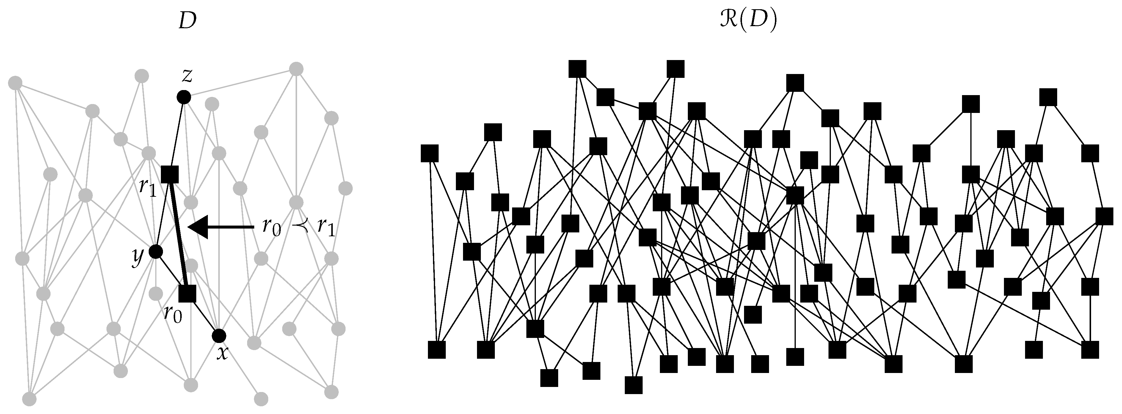
A gem of structural philosophy from pure mathematics is Grothendieck’s relative viewpoint, which emphasizes the study of objects together with their natural relationships. In discrete causal theory, the relative viewpoint is a conceptual tool of tremendous power and scope. A natural relationship between a pair of events in this setting is just a causal relationship, represented by a relation between elements x and y of a directed set . The collection of all such relations is just the binary relation ≺. It is surprisingly useful to view ≺ as a directed set in its own right, by recognizing “relations between pairs of relations”. The resulting object is called the relation space over D. Definition 5, adapted from Definition 5.1.1 of [14], generalizes this idea to multidirected sets.
Definition 5.
Let be a multidirected set, and let and be elements of its relation set R.
- 1.
- The induced relation ≺ on R is defined by setting if and only if .
- 2.
- The directed set is called the relation space over M.
The induced relation involves a new use of the precursor symbol ≺. Figure 4, adapted from Figure 5.1.3 of [14], illustrates the relation space over an acyclic directed set D. The left-hand diagram shows the construction of an individual relation , while the right-hand diagram shows as a whole. More generally, may be identified with the line digraph [32] over the directed multigraph corresponding to M. Theorem 6 gives the essential properties of relation space.
Theorem 6.
Passage to relation space defines a functor from the category of multidirected sets to the category of directed sets. This functor sends acyclic multidirected sets to irreducible acyclic directed sets, and preserves star finiteness.
Proof.
See [14], Theorem 5.1.4. ☐
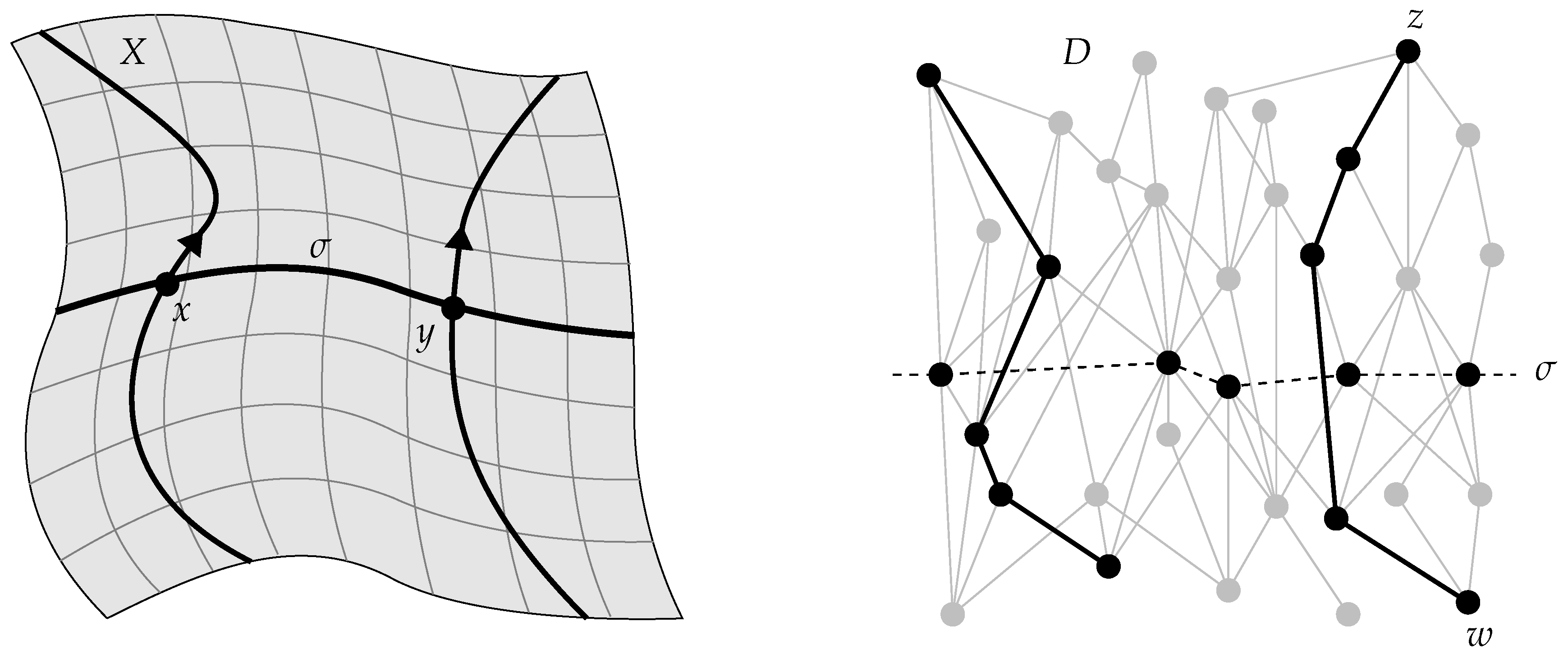
An important application of relation space in discrete causal theory is to eliminate a technical problem called permeability [33,34], which obstructs formulation and solution of initial value problems. In such a problem, one begins by specifying information associated with a maximal antichain in a directed set D, which is analogous to a spatial section of relativistic spacetime. One then attempts to solve for corresponding data throughout the future of . In general relativity, a Cauchy surface in a Lorentzian manifold X is an impermeable maximal antichain with respect to the causal structure of X, meaning that every inextensible causal curve in X intersects . Cauchy surfaces are useful for formulating initial value problems, because information cannot permeate a Cauchy surface to affect its future without being “filtered” by . Lorentzian manifolds containing Cauchy surfaces are called globally hyperbolic. The left-hand diagram in Figure 5, adapted from Figure 5.4.1 of [14], illustrates two causal curves intersecting a Cauchy surface in a globally hyperbolic manifold.
In discrete causal theory, a typical maximal antichain in a typical directed set D is permeable, meaning that chains in D may pass through from past to future without intersecting . In causal set theory [33], this phenomenon is referred to as “missing links”; the antichain is compared to a “sieve” [34], which is “by-passed” by a “large amount of geometric information”. “Thickened antichains”, obtained by adding limited quantities of past and future elements to , typically suffer from the same problem. Hence, maximal antichains are not good analogues of Cauchy surfaces in causal set theory, and the same statement applies to discrete causal theory in general. The right-hand diagram in Figure 5 illustrates a pair of chains permeating a maximal antichain in an acyclic directed set. The dashed lines connecting the elements of are a visual aid, not part of the structure. Permeability means that information can leak through , for example, from w to z. Besides posing a general obstacle to discrete causal dynamics, this problem also has as a specific bearing on the definition and analysis of entropic quantities, again typified in the causal set context [35,36]. Fortunately, however, this problem disappears upon passage to relation space.
Theorem 7.
Maximal antichains in relation space are impermeable. That is, if σ is a maximal antichain in the relation space over a multidirected set M, and if γ is a chain of relations in beginning at an element in the past of σ and terminating at an element in the future of σ, then γ intersects σ.
Proof.
See [14], Theorem 5.4.3. ☐
Path summation in discrete causal theory is described in terms of impermeable antichains, and therefore depends on the theory of relation space in an essential way.
2.4. Quantum Theory
Just as relations between pairs of events are central to discrete classical causal theory, so directed relationships between pairs of histories are central to discrete quantum causal theory. These relationships are called co-relative histories. The word “relative” refers to the relative viewpoint, while the prefix “co” derives from covariant constructions in category theory. The physical interpretation of a co-relative history is that it encodes the evolution of one history into another. The left-hand diagram in Figure 6, adapted from Figure 6.4.6 of [14], illustrates a family of four co-relative histories sharing a common initial history, called a cobase. The right-hand diagram illustrates how these co-relative histories are represented by morphisms of directed sets.
Individual morphisms in the category of directed sets do not always uniquely represent evolutionary relationships, due to symmetries. For example, the co-relative history in Figure 6 is represented by two different morphisms and , due to the symmetry interchanging the two maximal elements of its target history. Hence, co-relative histories are defined as equivalence classes of morphisms. It is convenient to restrict attention to special morphisms called transitions, which represent “growth” of directed sets. This idea is made precise in Definition 8, adapted from Definition 6.3.4 of [14]. Co-relative histories are then introduced in Definition 9, adapted from Definition 6.4.3 of [14].
Definition 8.
A transition in the category of directed sets is a monomorphism , embedding its source D into its target , , as a proper, full, originary subobject. Here, “proper" means that has nontrivial complement in , “full" means that in if and only if in D, and “originary" means that the isomorphic image of D in contains its own past.
At a less-formal level, the condition that is a monomorphism means that does not “erase” details of the source D. The “proper” condition means that encodes nontrivial change. The “full” condition means that does not “edit” details of D. The “originary” condition means that does not add “prehistory” to D. These conditions support the desired evolutionary interpretation.
Definition 9.
A proper, full, originary co-relative history is an equivalence class of transitions , where two transitions τ and are equivalent if and only if there exists an automorphism β of mapping onto . The common source of the transitions representing h is called the cobase of h, and the common target of these transitions is called the target of h.
The subscripts i and t in the expression stand for “initial” and “terminal”. This notation is different from the notation for arbitrary transitions in Definition 8, since Section 3 and Section 4 feature auxiliary transitions related to h that do not belong to the equivalence class defining h. The proper, full, and originary conditions in Definition 9 allow the unadorned term “co-relative history” to mean something more general, but co-relative histories in this paper always satisfy these conditions, except in the context of superset microstates in Definition 15, where they need not be full. Each transition in the equivalence class defining h is said to represent h. The “double arrow” notation ⇒ emphasizes that h may be represented by more than one transition, but often h is uniquely represented due to the rigidity of typical “large” directed sets [37], which plays an important role in Section 3 and Section 4. It is useful to think of h as “adding elements and relations to to produce ”, but one cannot always identify specific elements and relations as “the ones added” since h is an equivalence class. Multiple inequivalent transitions, and hence multiple co-relative histories, may exist between a given pair of directed sets, even a pair differing by a single element. This implies multidirected structure at the quantum level.
Choosing a suitable family of directed sets, together with a suitable family of co-relative histories between pairs of members of , one obtains a structure called a kinematic scheme, which serves as a history configuration space. The word “kinematic” means that encodes possible behavior, without identifying what specific behavior is determined or favored under specific conditions. The latter question involves dynamics. As an analogy, relativistic kinematics describes possible particle paths, e.g., ruling out spacelike motion, but the paths of specific particles depend on dynamical information. possesses natural multidirected structure induced by , elaborated below. Sequences of co-relative histories in define evolutionary pathways called co-relative kinematics, abstractly analogous to particle paths in conventional path summation. The conditions that must satisfy to qualify as a kinematic scheme are that must include enough co-relative histories to describe the evolution of any history in , and must contain all “ancestors” of its members. These conditions are made precise in Definition 10, adapted from Definitions 7.4.1 and 7.4.7 of [14]. An additional desirable property, called the generational property, allows each co-relative history in to be “factored into generations”. However, this property is not studied in this paper, and it is preferable to omit it from the definition.
Definition 10.
A kinematic scheme is a pair , where is a class of directed sets, and is a class of co-relative histories between pairs of members of satisfying the following properties:
- 1.
- Accessibility: If D is in , then there exists a sequence of co-relative histories in terminating at D.
- 2.
- Hereditary property: is closed under the formation of proper, full, originary subobjects.
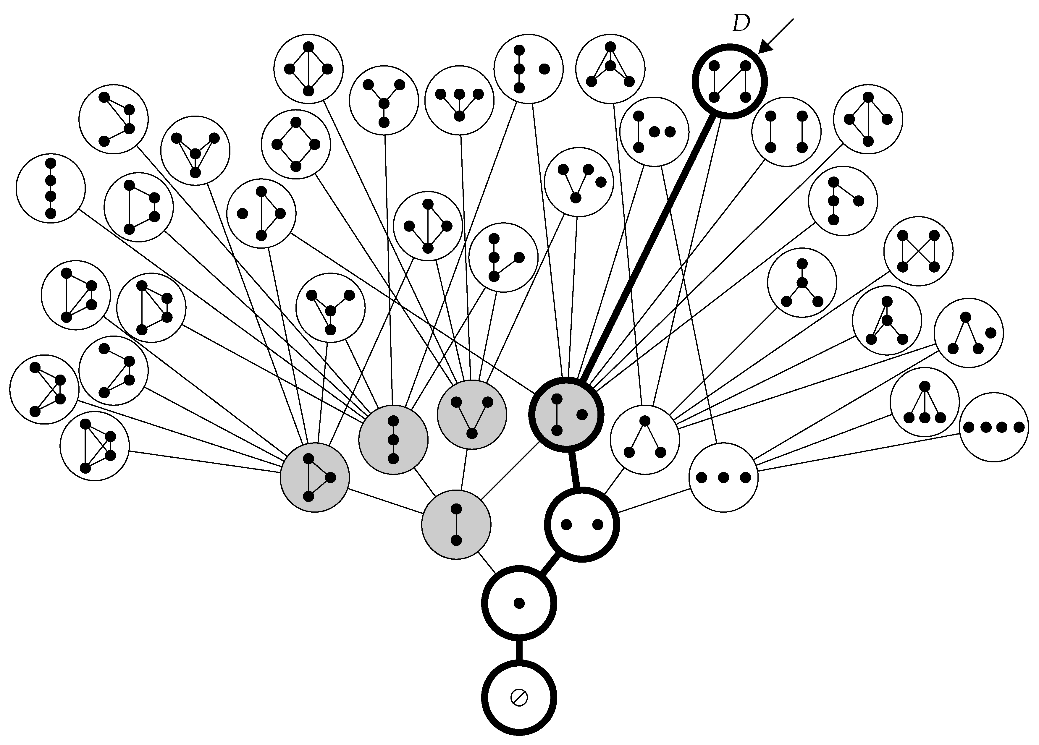
Figure 7, adapted from Figure 7.5.2 of [14], illustrates a portion of a kinematic scheme called the positive sequential kinematic scheme, which serves as a source of examples throughout the remainder of the paper. is modeled after a kinematic scheme of finite causal sets appearing implicitly in Sorkin and Rideout’s theory of sequential growth dynamics [38]. Similar structures appear elsewhere in the work of Sorkin [39], Isham [40,41,42,43], Markopoulou [7], and others. The objects illustrated inside each large open node in the figure are members of the class of directed sets of , which is the class of finite acyclic directed sets. This class is more restrictive than the class specified by Definition 4, which requires only countability. The edges connecting the large open nodes represent members of the class of co-relative histories of , which are those that “add a single new element to their targets”. This means that if belongs to , and if is a transition representing h, then the complement of in is a singleton. The gray-colored nodes illustrate how the set of four co-relative histories appearing in Figure 6 embeds into . The thickened edges illustrate a co-relative kinematics in , whereby the empty set ⊘ evolves into a directed set D with four elements and three relations. The specific transition or transitions representing each co-relative history illustrated in the figure may be inferred in a straightforward manner from the directed structures of its cobase and target; for example, there is a unique transition representing the final co-relative history in the co-relative kinematics terminating at D. The “new element added by ”, i.e., the complement of the image of , is the top-right element indicated by the arrow.
Given a kinematic scheme , it is useful to associate an abstract multidirected set with , where each member D of is represented by an element of , and where each member of is represented by a relation from to in . is called the underlying multidirected set of . Chains in represent co-relative kinematics in . The left-hand diagram in Figure 8, adapted from Figure 7.5.4 of [14], illustrates a portion of the underlying multidirected set of the positive sequential kinematic scheme . The chain from to represents the co-relative kinematics from ⊘ to D illustrated in Figure 7. This diagram illustrates the permeability problem in the context of kinematic schemes; the three nodes connected by the auxiliary dashed lines represent a maximal antichain in , which is permeated by the chain from to . It is therefore necessary to work in relation space to properly formulate the theory of path summation. The right-hand diagram in Figure 8 illustrates part of the relation space . The dark square nodes represent a maximal antichain, which is impermeable by Theorem 7.
While one could choose to perform path summation over a particular acyclic directed set, the resulting theory would be background dependent, and hence unsuitable for quantum gravity. Path summation in the background independent context involves summing phases associated with co-relative kinematics in a kinematic scheme . As explained in Section 1.4, these phases are analogous to Feynman’s phases . Under modest assumptions, is a product of phases of individual relations representing individual co-relative histories. The relation function determines a specific form for Equation (4)
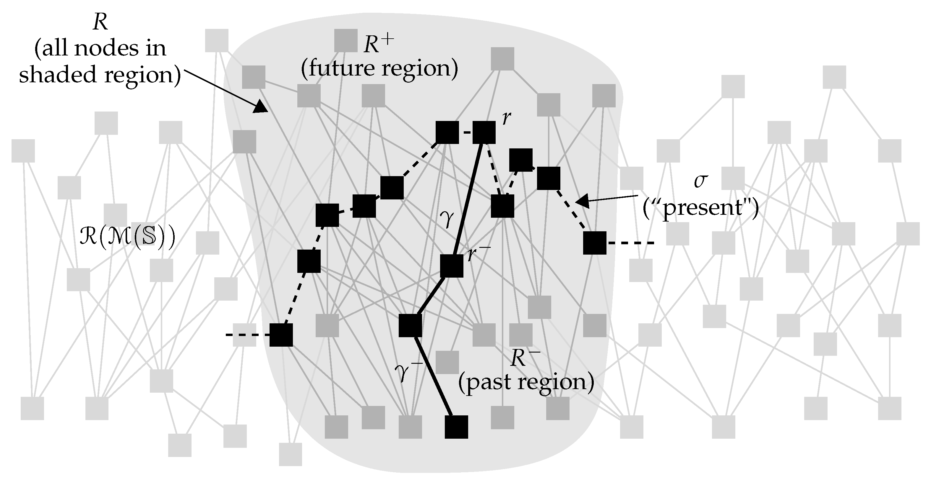
reproduced here for convenience. The setup for deriving this equation is illustrated in Figure 9, adapted from Figure 6.9.2 of [14], where the derivation is carried out in detail. The auxiliary shading represents a finite subobject R of the relation space . A choice of maximal antichain partitions R into a disjoint union , where represents a choice of “present”, and are the corresponding past and future regions. The function is called the past state function, because it depends on all chains in , which terminate at elements of . Here, one such chain is shown, terminating at an element , with penultimate element . This chain may be factored into a concatenation product , where is the subchain of terminating at , and this factorization induces a factorization of phases. The value is defined to be the sum of the phases of all maximal chains in terminating at r. Mathematically, Equation (4) merely organizes the factorizations for all such . These chains represent co-relative kinematics in the corresponding region of that lead to the target history of the co-relative history represented by r. Generalizing to the case of infinite R raises questions of convergence. From an abstract perspective, the function plays a role similar to that of Feynman’s “wave function” ([1], Section 5), except that no limiting process is necessary to define it, and no normalization constant is required. However, the structural context in which arises is much different than in Feynman’s original non-relativistic background dependent setup, where evolutionary pathways are represented by paths in a fixed copy of . In the present discrete background independent context, each step along a chain represents a co-relative history, interpreted as the evolution of one spacetime into another. Equation (4) describes how the value of changes when the evolutionary pathways involved are extended by one additional relation r, which corresponds to multiplying the associated phases by . Abstractly, it arises in almost the same manner as the ordinary Schrödinger equation under Feynman’s derivation ([1], Section 6), in which segmented paths approximating continuous evolutionary processes are extended via a time-stepping method. For Equation (4), however, no approximation is involved, so no limiting process is necessary.
A few further remarks regarding Equation (4) may be helpful. First, it is illuminating to spell out how the equation can describe quantum-theoretic behavior specifically. This depends partly on the general properties of path summation, and partly on the choice of relation function that determines the phase associated with each evolutionary pathway. Like virtually any formula involving path summation over a history configuration space, Equation (4) combines contributions from many distinct processes involving many distinct histories. This is a familiar feature of quantum-theoretic superposition, but is not unique to the quantum realm. For example, classical stochastic models such as Sorkin and Rideout’s theory of sequential growth dynamics [38] organize information in a similar manner at an abstract level, but are decidedly non-quantum. The classical nature of the latter theory arises from the assignment of real probabilities, rather than quantum amplitudes, to evolutionary pathways. Similarly, Feynman’s derivation [1] could just as easily be used to produce a continuous classical stochastic model, with real probabilities assigned to subspaces of a path space. What leads to Schrödinger’s equation specifically under Feynman’s setup is Feynman’s choice of phase map, which produces the type of interference effects necessary to describe quantum-theoretic behavior. Similar considerations apply in the discrete causal context. For different choices of , Equation (4) could be used to describe a classical stochastic model, or a quantum-theoretic model, or neither. This highlights why the choice of phase map is so crucial to the theory. As described in Section 1.4, the most obvious choice of target object for a quantum-theoretic phase map is the choice made by Feynman, namely, . Alternative choices can be interesting, but this paper focuses on -valued phase maps almost exclusively. Second, due to the quantum-gravity-related focus of this paper, it is worth noting that Equation (4) shares certain similarities with the Wheeler-Dewitt equation, but these are not explored here. Third, allowing cycles complicates the picture, and this generalization is not considered here. Fourth, many different kinematic schemes typically share a given class of directed sets, and different schemes offer different perspectives regarding the evolution of families of histories. Physical predictions must be independent of these choices, and this is expressed by saying that the theory must be covariant. In practical terms, this means that if one changes , then one generally must change to compensate. This paper mostly ignores covariance issues.
Figure 10 illustrates a sequential growth process in , in which a history with seven elements evolves into a history with eleven elements via a sequence of co-relative histories labeled to . These co-relative histories are represented by relations to in , abbreviated by to . This growth process serves as a source of examples in Section 3 and Section 4. Each pair of consecutive histories in Figure 10 encodes the same type of information associated with a single square node in Figure 9, since these nodes represent co-relative histories. Given such a process, the goal is to define phases measuring the “favorabilities” of each co-relative history. The black nodes and edges represent the first-degree terminal states to of the histories to , which encode the first-order information in each history, i.e., the “physically new” information, consisting of only the most recent causes and effects. First-degree terminal states are featured repeatedly in Chapters 7 and 8 of [14], where they are described via terminology such as “structural increments” or “generations”. By definition, only one element in each history is “new” from the perspective of the sequential growth process itself; these new elements are indicated by arrows. However, this process is merely one way of describing the evolution of , and therefore involves arbitrary extraphysical choices regarding the order of appearance of elements. Terminal states of degree n are introduced in Definition 13. For , there is a distinction between degree and order; for example, second-degree terminal states may encode information of arbitrarily high order. It is convenient to use the abbreviation for , which highlights the fact that is a “structural increment” of . To avoid clutter, only is labeled in the figure. The symbol is used in later sections to denote states of arbitrary degree.
First-degree terminal states are analogous to “present states” in conventional physics, involving data up to first order, such as position and velocity. Familiar notions of entropy are associated with such “present states”, not with entire histories. In particular, the second law of thermodynamics compares the entropy of a “present state” to that of “previous states”; it does not involve a “higher-dimensional entropy” associated with the entire history leading up to the present state. The evolution of physical systems does not seem to be sensitive to details of the distant past; otherwise, one could not perform reliable experiments without knowing the exact history of each piece of experimental equipment. More formally, Lagrangians are typically assumed to depend on information only up to first order. The form of Equation (4) imposes an analogous assumption at the level of kinematic schemes, since the relation function is analogous to a Lagrangian on . As discussed in Section 3.3, higher-order information at the level of individual histories is not a priori irrelevant in discrete causal theory, but contributions from the distant past likely play a negligible dynamical role. Hence, the simplest “serious" entropic phase maps are defined in terms of first-degree terminal states, and more-sophisticated phase maps may be regarded as refinements of such maps.
3. Entropy and the Second Law of Thermodynamics
3.1. Entropy
Entropy, in the statistical sense pioneered by Boltzmann, may be understood very generally in terms of the distinguishability of objects described at two different levels of detail, one regarded as fine, and the other regarded as coarse. The prototypical application of this idea occurs in statistical thermodynamics, in which the fine level of detail for a system, such as a fixed quantity of ideal gas, is described in terms of microscopic data, such as the positions and momenta of individual molecules, while the coarse level of detail is described in terms of macroscopic data, such as pressure, volume, and temperature. Each possible choice of macroscopic data defines a coarse description of the system, called a macrostate, while each possible choice of microscopic data defines a fine description, called a microstate. Each macrostate generally corresponds to many different microstates, since many different choices of microscopic data may be approximated by identical macroscopic data. The entropy of a macrostate measures the quantity of corresponding microstates in a manner that is additive for composite systems. In more general terms, objects distinguishable at some fine level of detail may be indistinguishable at some coarser level, and a notion of entropy may be associated with the two levels to quantify this difference in distinguishability. In particular, generalizations of Boltzmann entropy such as Gibbs, Shannon, and Rényi entropies fall under the same conceptual umbrella. Measures of entropy familiar in ordinary quantum theory, such as von Neumann entropy, are less relevant, since they depend on specific algebraic apparatus less general than the path summation approach.
In statistical thermodynamics, the state space for a system is an abstract space parameterizing the set of possible microstates of the system for some choice of fine detail. A choice of coarse detail partitions state space into a family of subsets representing the possible macrostates of the system, where the points of each subset parameterize the microstates associated with the corresponding macrostate. Such a partition is called a coarse-graining of the state space. The left-hand diagram in Figure 11 illustrates such a coarse-graining, where the cells representing macrostates are separated by solid lines. Dotted lines and labels are explained below. Such a planar diagram could be interpreted literally as encoding the possible position and momentum of a single particle moving in one real dimension, but all such diagrams in this paper are schematic. Conventional state spaces are real manifolds, and therefore exhibit notions of proximity, volume, and other topological and metric structure. However, their dimensions are typically quite large, and this implies properties that are not well-represented by planar diagrams; for example, each region typically has very many neighbors. Even in 24-dimensional Euclidean space, each sphere in the regular packing induced by the Leech lattice is tangent to neighbors; one may imagine the situation in -dimensional space. Abstract metric-related ideas remain useful for describing the properties of discrete causal state spaces, but planar diagrams only roughly represent these notions.
Generalizing the thermodynamic picture, any set S of objects may be partitioned into a family of subsets P, where the objects belonging to each subset are regarded as equivalent at a coarse level of detail. More generally still, one may consider a strictly partially ordered family of partitions of S for some index set A, where by definition if and if every member of is a union of members of . In this case, is called a refinement of . Here, ≺ does not represent causal structure, and superscript indices are used to distinguish information filtering from mere enumeration. One may define equivalence relations on S for each in A, where if s and belong to the same subset under . If , then induces a quotient partition of the quotient set in an obvious way. Any such choice of and may be used to define notions of coarse and fine detail. Returning to Figure 11 in this more abstract setting, the large regions bordered by solid lines in the left-hand diagram represent a choice of coarse detail for a set S, while the small regions bordered by dotted lines represent a choice of fine detail. Here, and each partition S into subsets of roughly equal size, but a typical coarse-graining in conventional thermodynamics exhibits vast differences in the sizes of regions, and correlations exist involving proximity and size. The middle diagram in Figure 11 illustrates such a coarse-graining. As emphasized by Penrose [44], such details are crucial for understanding whether a typical system can be expected to exhibit a systematic increase in entropy. For example, the right-hand diagram in Figure 11 illustrates a state space that induces an “inverse second law of thermodynamics”, in the sense that a typical path in this space moves from larger to smaller cells. If , and if each member of is a finite union of members of , then one may define multiplicities and entropies via counting: if is a member of , and if for members of , then the multiplicity of V is K, and the entropy of V is . The choice of notation for and is intended to emphasize the relative viewpoint: multiplicities and entropies are properly understood in terms of natural relationships between levels of detail, not in terms of any specific level of detail. For the set V shown in the left-hand diagram in Figure 11, the entropy is , since subdivides V into seven regions. In more general settings, it may be necessary to measure the sizes of members of via some measure other than the counting measure.
Definition 11.
An entropy system consists of a set S, a set of partitions of S for some index set A, strictly partially ordered by refinement, and a family μ of measures on the quotient sets , one for each relation in Π. Each such relation induces an entropy quadruple . The entropy of a member V of is , where is the image of V under the quotient map , and where is understood to mean ∞.
It is often convenient to denote an entropy quadruple by just S, or to write to indicate that a set S is equipped with such a structure. The functions are taken to be measures here for simplicity, but the situation could be generalized further. In particular, the target object of need only be a totally ordered set. One may also abstain from using logarithms to “rescale” . However, it suffices here to consider only the counting measure on a finite set or the Lebesgue measure on a finite-dimensional real manifold, and logarithms are useful for producing quantities that are additive for composite systems. The reason for using “e” instead of the familiar “h” for entropy is because “h” is used here to represent co-relative histories. Figure 12 illustrates a simple entropy system whose underlying set S is the unit interval in . The set of partitions of S has members , , , and , which subdivide S into segments of equal lengths 1, , , and , respectively. is the trivial partition, under which S represents a single macrostate. The strict partial order ≺ on consists of five individual relations , , , , and , each of which induces an entropy quadruple. The quotient sets , , , and have 1, 2, 3 and 6 elements, respectively. There are two nontrivial quotient partitions, and , which subdivide the quotient set into equal-sized subsets with 3 and 2 elements, respectively. Multiplicities and entropies of some representative subsets of S with respect to different entropy quadruples are also listed. For example, the subset of S has measure and entropy with respect to the entropy quadruple .
The motivation for adopting such a general viewpoint is that multiple “levels” of entropy are evident in discrete causal theory. An important example involves the nth-degree terminal states mentioned in Section 2.4 and formally introduced in Definition 13. Given two directed sets D and , it may be the case that and are isomorphic, while and differ. In this case, D and are indistinguishable at the level of detail specified by the index value n, but become distinguishable at the finer level of detail specified by the index value . On the level of individual elements, two elements x and y belonging to a subobject of a directed set D may be “locally indistinguishable”, in the sense that they are interchanged by an automorphism of , but may be “globally distinguishable”, in the sense that no such automorphism extends to an automorphism of D. More generally, one may consider chains of subobjects containing x and y, some of which possess automorphism groups interchanging x and y, and some of which do not. Of obvious interest is the case in which is a low-order terminal state of a history, and for are progressive “thickenings” of .
While entropy is defined by associating entire families of “fine” states with individual “coarse” states, it is sometimes interesting to compare the amount of detail encoded by specific pairs of states. It is then natural to relate such “local comparisons” to the “global comparisons” leading to entropy systems. In this context, one need not distinguish a priori between macrostates and microstates; states are defined individually by specifying varying degrees and types information about an object or system, and are then compared and categorized. Given two such states and , it is sometimes possible to unambiguously identify as more detailed than , or vice versa. In other cases, and are incomparable, in the sense that contains more of one type of information, while contains more of another. In this setting, one may recognize a natural partial order ≺ on the family of states under consideration, where if and only if is unambiguously more detailed than . This type of partial order is different from the partial orders on sets of partitions in Definition 11, but the two types of structure are related. For example, given an entropy quadruple , the set is a subset of the power set of all subsets of S. The relation means that every member V of is a union of members W of . One may define an induced relation on , also denoted by ≺, where if and only if V is a proper superset of W. Hence, a single relation between two partitions induces a partial order on a corresponding family of subsets. This partial order is of a special type, with maximal chain length 1, because its only relations are those of the form for and such that . However, one may easily define partially ordered sets with longer chains by considering sequences of partitions
Working in the opposite direction, one may begin with a partial order ≺ on an arbitrary set . Here, is viewed as an abstract analogue of a family of states encoding various types and quantities of detail, while ≺ is viewed as an abstract analogue of the partial order relating pairs of states and whenever is unambiguously more detailed than . One may partition into a family of antichains with respect to ≺. There are generally many different choices of partition, each analogous to a frame of reference in relativity. In the entropic setting, elements of a given antichain are viewed as abstract analogues of states sharing an equal level of detail. In the simplest case, the antichains “foliate” , in the sense that each nonextremal antichain has an unambiguous maximal predecessor and minimal successor . More generally, the antichains form a partially ordered family. In either case, the partition defines an atomic decomposition of with respect to ≺, an idea revisited in a different context in Section 3.3. In many cases, detail may be quantified in a variety of different ways, and this leads to the consideration of families of partial orders on . Such families are themselves partially ordered via the order-theoretic version of refinement, under which precedes if and only if whenever . An antichain with respect to is then automatically an antichain with respect to , so any partition of induced by refines at least one such partition induced by . In this manner, the partial ordering by refinement of the family of partitions induced by respects the partial ordering on itself. Hence, entropy systems defined in terms of such partitions automatically respect the order-theoretic structure of .
3.2. The Second Law
The familiar intuition regarding the second law of thermodynamics is that “entropy increases with time”. Generalizing this idea to apply to the broad framework of entropy systems introduced in Section 3.1 requires suitable analogues of “time” and “increase”. Time evolution is conventionally represented by a directed curve in state space, and in this context the second law says that motion along such a curve tends to pass from smaller to larger cells in a specified coarse-graining. The left-hand diagram in Figure 13 illustrates such a curve . A typical curve originating in one of the two shaded areas is likely to exhibit a systematic increase in entropy, at least for early times, since such curves begin in small cells whose borders are dominated by larger cells. A typical curve originating elsewhere in the state space does not exhibit such an increase in entropy. This illustrates the fact that both the structure of state space and the region of origin of the curve describing the system of interest are relevant to the existence of a recognizable second law. In the cosmology of the early universe, for example, the question of why specific measures of entropy were initially relatively low is just as important as the question of why entropy increased thereafter [44].
The abstract analogue of a directed curve in state space is a map from a linearly ordered set L into an entropy quadruple . Such a map is illustrated in the right-hand diagram in Figure 13. Here, L is drawn to suggest an interval in , but in more general settings L may be a non-continuous object such as an interval in , a discrete object such as an interval in , a finite object such as the set , or even a transfinite object, such as the long line. The notion of an increasing function requires similar generalization beyond the familiar setting of real analysis. Even in conventional thermodynamics, strict definition of an increasing function must be relaxed, since the second law is understood not as a prescription that entropy must increase over any time interval, but as a description of the fact that entropy does increase with overwhelming likelihood over sufficiently long time intervals. The map in the figure passes through cells of multiplicities 5, 2, 3, 7, 6, 6, 7 (again), 4, 2, 4, and 6 (again). Hence, the associated system does not obey a discernible version of the second law. In the general case, it seems preferable to describe a variety of ways to define a version of the second law for such a system than to isolate a particular choice via formal definition. An individual map from a totally ordered set L into an entropy quadruple , obeys a strict version of the second law if for every pair of subsets V and of S belonging to , and for every pair of elements ℓ and in L such that and , it is true that . Intuitively, this means that never passes from a large cell into a smaller cell. There are various ways to relax this strict description. If L possesses a metric, then one may specify a rule relating the size of the interval to the probability that . If the target object of also possesses a metric, then one may define something like a derivative, i.e., a rule relating the sizes of the intervals to the sizes of the corresponding intervals . More generally, a region U of S obeys a version of the second law if a typical map originating in U obeys an individual version of the second law. The word “typical” may be made precise in terms of a generalized measure on the space of maps . It is sometimes necessary to restrict attention to special maps to obtain a clear pattern; for example, some entropy quadruples exhibit entropy increases along typical “short curves”, but not along typical “long curves”. In particular, some cosmological models posit a reversal of the second law in the distant past and/or future.
3.3. Discrete Causal State Spaces
In statistical thermodynamics, microstates are determined by information up to first order, e.g., by positions and momenta of individual molecules. Such information, together with the dynamical laws of classical mechanics, is sufficient to recover higher-order information; one may uniquely evolve a given state “backward in time”. Hence, if two states are indistinguishable up to first order, then they are absolutely indistinguishable. In discrete causal theory, the situation is different. The analogue of information up to first order in a finite acyclic directed set D is its first-degree terminal state , which consists of all maximal elements of D, all relations terminating at these elements, and all initial elements of these relations. Knowledge of generally does not enable recovery of D. One may propose a choice of classical dynamics implying such a relationship for very special classes of directed sets, for example, by abstracting the Einstein–Hilbert action from general relativity, which takes the form
in the simple vacuum case with zero cosmological constant. Here, g is a Lorentzian metric on a 4-dimensional manifold X, R is the curvature scalar arising from the metric connection, G is Newton’s gravitational constant, and c is the speed of light. Yet despite interesting efforts in this direction, for example, in causal set theory [45,46,47], such a strategy is dubious due to the amount of geometric structure taken for granted in relativity. Geometric data such as metrics and curvature, and even “pre-geometric” data such as dimension and topology, are emergent notions in discrete causal theory. Action functionals in this context must be defined more fundamentally, and cannot be expected to produce straightforward analogues of deterministic, time-symmetric Euler–Lagrange-type equations that uniquely determine classical dynamics via information up to first order. In particular, elements of a directed set D that are indistinguishable up to first order, i.e., permuted by an automorphism of , may be distinguishable when one considers higher-order information. It is therefore necessary to consider higher-degree terminal states in what follows. The form of Equation (4) does assume that first-order information suffices at the level of kinematic schemes, in the sense that the phase of an arbitrary co-relative kinematics is the product of the phases of its individual co-relative histories. This picture may be generalized without leaving the general framework of path summation, but such generalization is not undertaken here. In any case, the latter phases do generally depend nontrivially on information above first order in the corresponding cobases and targets.
The simplest discrete causal analogues of familiar thermodynamic state spaces are nth-order state spaces , whose elements represent isomorphism classes of countable star finite acyclic directed sets with maximal chain length n. Equivalently, is a nonempty antichain. It is useful to preface formal definitions involving with some informal remarks. First, while the notion of order identifying a state as a member of is intrinsic to itself, the desired interpretation of is as a terminal state of a history D, containing information encoded by chains of length at most n terminating at maximal elements of D. Second, it is usually impossible to choose a member of that includes all such information for , because chains of length at most n terminating at different maximal elements of D may intersect to produce longer chains, thereby defining a higher-order state. One might consider re-defining to include such states, requiring only that each element be connected to a maximal element by at least one chain of length at most n. In physical terms, such states are still composed of elements exerting “recent influence”, but may contain chains of arbitrary length. However, such a definition would not be ideal for the desired applications. For example, it would allow any countable star finite acyclic directed set in which all chains are bounded above to be converted to a member of or by adding new relations terminating at new maximal elements, thereby flouting the intuition that low-order states should be “causally simple”. It is preferable to define a separate notion called degree, which facilitates the definition of terminal states containing all information up to a given order in a particular history. Following this idea, Definition 13 introduces special states , called nth-degree terminal states, which include all information encoded in chains of length at most n terminating at a maximal element in D. Third, as mentioned in Section 2.4, the distinction between order and degree does not arise for ; the first-degree terminal state of D automatically belongs to . Fourth, the nth superset microstates introduced in Definition 18 are constructed by adding n “prehistorical” elements to a state, which may not increase its maximal chain length at all. These subtleties reflect the fact that more than one natural-number grading is useful in studying discrete causal state spaces.
It is useful to define terminal states in terms of transitions between pairs of histories, using the relative viewpoint. Though the ultimate goal is to use information encoded in terminal states to assign phases to sequences of co-relative histories, i.e., co-relative kinematics, the states of principal interest in studying a given co-relative history are typically not those induced by transitions representing h. This is because the “physically new” structure associated with and is more meaningful than whatever structure h “adds to” to produce . For example, each co-relative history in adds only one element to , so most of the physically new structure in is typically already present in . Yet what one is really interested in is whether or not the physically new structure in is “more favorable” than the physically new structure in ; i.e., one wishes to compare terminal states of and . These may be defined in terms of auxiliary transitions that are determined by h, but do not represent h under Definition 9. First, however, one must define terminal states associated with arbitrary transitions.
Definition 12.
Let be a transition of acyclic directed sets. The subobject of consisting of all elements of , all relations terminating at such elements, and all initial elements of such relations, is called the terminal state of τ. If is a nonempty antichain, then the order of is n.
Despite the relative nature of Definition 12, it is convenient to refer to as a terminal state of the target set in many cases. does not include relations between elements of ; it includes only relations that are “new” with respect to . If the context is expanded to include cycles, a different definition of order is necessary. For example, one may define to be the maximal length of non-self-intersecting chains in . Here, however, I focus almost exclusively on the acyclic case. Any directed set is itself the terminal state of the unique transition . This transition may be denoted by when the choice of target set is obvious. As mentioned above, is useful to define special terminal states that encode all information up to order n in a given history.
Definition 13.
Let D be an acyclic directed set in which every chain is bounded above.
- 1.
- The nth-degree terminal state of D is the subobject of D consisting of all elements connected to a maximal element of D by a chain of length at most n, together with all relations in such chains.
- 2.
- The nth-degree initial state of D is the subobject of D constructed by deleting all non-minimal elements of from D, together with all relations in D terminating at such elements.
- 3.
- The nth-degree transition associated with D is the inclusion map .
The boundedness hypothesis in Definition 13 is included to rule out situations in which D has maximal elements but also has chains “extending to infinity”, since it is awkward to exclude such chains from consideration when studying terminal behavior. Such histories are not considered here.
Definition 14.
The nth-order state space is the set of all isomorphism classes of countable star finite acyclic directed sets Δ such that is a nonempty antichain. The finite-order state space is the disjoint union , and the (total, countable, acyclic) state space is the set of all isomorphism classes of countable acyclic directed sets, which may be viewed as limits of sequences in .
Since the elements and relations in a member of are assumed to possess no internal structure, one might expect to be treated as a microstate. However, since discrete causal theory does not rule out the dynamical relevance of information above order n at the level of individual histories, data describing how might fit into a larger history can be important in determining future behavior influenced by . Such data defines an even finer level of detail than itself, permitting to be viewed as a macrostate. Ambiguity regarding the status of is not surprising, due to the relative nature of entropy. Figure 14 illustrates four different methods of defining coarse and fine levels of detail using . Informal discussion of these methods then precedes formal treatment in Definition 15. The first diagram shows a third-order state embedded in a history D. In this case, does not contain all the third-order information in D; in particular, it is not the third-degree terminal state of D. The second diagram illustrates one way to treat as a microstate, called a resolution microstate, by approximating its structure via the method of causal atomic resolution, introduced in [14]. This method involves choosing special subsets of , called causal atoms, which serve as individual elements of a coarser directed set. Such a choice defines a causal atomic decomposition of . A sequence of such decompositions is a causal atomic resolution, with each subsequence defining “initial” and “terminal” levels of detail, and hence a notion of entropy. More generally, one may define partially ordered families of decompositions, also called resolutions, which induce entropy systems. The resolution in the figure involves a single decomposition, and hence just two levels of detail. Causal atomic resolution provides perhaps the most obvious discrete causal analogue of conventional coarse-graining. In particular, it involves actual approximation, meaning that the information contained in a causal atomic decomposition is not only incomplete, but also imprecise. However, there is generally no canonical choice of resolution for a given state, and different resolutions may be very dissimilar. Further, resolutions reaching far above the fundamental scale can produce objects that are obviously “too granular” to resemble physical spacetime. Members of are usually treated as macrostates in this paper, but methods such as causal atomic resolution remain worthy of further study in more general entropic settings.
The third diagram in Figure 14 illustrates the most obvious way to treat a member of as a macrostate, by adding “prehistory” to define larger states called superset microstates. Different superset microstates of impose different constraints on the family of histories of which could be a terminal state. In particular, the superset of shown in the diagram is induced by the history D. At a higher level of detail, may itself be viewed as a macrostate, with its own superset microstates adding more prehistory. One may imagine “flipping over” this diagram to obtain a co-relative history between the causal duals and of and , and this is how superset microstates are formalized in Definition 15. Hence, the convenient term “superset” is not quite precise, because co-relative histories involve equivalence classes. Naïve amalgamation of superset microstates produces a state space with an infinite number of elements in each cell, since one may always add more prehistory to a directed set. This leads a priori to infinite multiplicities and entropies for finite states. However, supersets adding “recent” data are expected to dominate dynamically, and families of superset microstates may be filtered to reflect this expectation. In the case of finite states, one may work with finite families of microstates defined in terms of numbers of elements and relations, lengths of chains, sizes of antichains, and similar quantities. Here, I focus on families defined via the number of prehistorical elements added to . The quantity of superset microstates of a given type is decreased by symmetries of , which render equivalent different subsets of . This meshes with the intuition that high-entropy states should be “disordered”. For example, if is an antichain of cardinality K with automorphism group , then there is only one way to add a single prehistorical element and k relations to for any , since the terminal elements of these relations in may be exchanged for any other k elements of under . By contrast, there are ways to add such an element and relations to if is trivial.
The fourth and fifth diagrams in Figure 14 illustrate contrasting ways to treat a member of as a macrostate by focusing on its symmetries directly. Under the method illustrated in the fourth diagram, a microstate of is simply a copy of labeled via a map , where L is a set of consecutive natural numbers starting with zero, and where two labelings are regarded as equivalent if they are related by an automorphism of . Such a microstate is called a labeled microstate. The number of labeled microstates associated with a state of cardinality K ranges from 1 if to if is trivial. This method agrees qualitatively with the superset approach in the sense that high-entropy states are those for which is small. The method illustrated in the fifth diagram essentially reverses this relationship. Here, one begins with an arbitrary labeling , where is the subset of not fixed by . Automorphisms of convert ℓ to other labelings, each of which represents a symmetry microstate. Such a microstate may be viewed as a “mode of symmetry breaking”, since it breaks the symmetries of in a specific way. For a finite state , the number of symmetry microstates is just , so high-entropy states are those for which is large. More generally, one may work with non-surjective partial labelings that leave a subgroup of unbroken. The labeling in the figure is of this type, since there remains an automorphism of interchanging the elements indicated by arrows. The set of such partial labelings is partially ordered by extension, which is interesting from the perspective of state-specific detail discussed at the end of Section 3.1. While it is counterintuitive to associate high entropy with symmetry, there are arguments for entertaining such possibilities. Symmetry is central to the theory of “elementary” particles, so certain special structures that are locally symmetric, at least at measurable scales, are favored by the actual dynamics of the physical universe. Such structures may be “attached” to underlying causal structure via auxiliary algebraic information, but the strong interpretation of the causal metric hypothesis demands an emergent description of both spacetime symmetries and internal symmetries. The most obvious way to satisfy this demand is to incorporate some type of symmetry data directly into Equation (4). Notions of entropy associated with superset microstates and/or labeled microstates might accomplish a similar purpose, since their enumeration depends largely on symmetry considerations. Regardless of the type of entropy chosen, an attractive though speculative idea is that elementary particles might arise via local entropic traps, whereby certain regular structures that are small by conventional measures but large compared to the fundamental scale might be very stable from an entropic perspective.
A mathematical result important in the study of superset microstates, labeled microstates, and symmetry microstates is Bender and Robinson’s proof [37] that a typical acyclic directed set D has trivial automorphism group, i.e., is rigid. This result applies asymptotically under modest assumptions about the number of relations in D. However, these assumptions fail to hold for a typical low-order terminal state , since such a state has unusually large “spatial size” and small “causal size”, and typically lacks enough relations to “bind elements in place”. Hence, is often nontrivial for such a state. The extreme case is a zeroth-order state, whose automorphism group is the entire symmetric group permuting its elements transitively. However, states tend to become increasingly rigid as their order increases. Bender and Robinson’s result enables rough enumerations of the number of high-order superset microstates and labeled microstates for a state of a given cardinality. It also suggests a novel explanation for why the details of the distant past seem to be irrelevant to future dynamics, namely, because relatively few additional generations of elements must be added to a typical low-order state to break most of its symmetries.
Definition 15.
, , and may be used to define finer state spaces, for which their members are macrostates.
- 1.
- The nth-order superset state space is the set of full, originary co-relative histories . where Δ is a member of and is a member of . Its elements are called superset microstates. The corresponding finite-order superset state space and (total, countable, acyclic) superset state space are defined in the obvious ways.
- 2.
- The nth-order labeled state space is the set of complete labelings of members Δ of , where two labelings of Δ are considered to be equivalent if they are related by an element of . Its elements are called labeled microstates. The corresponding finite-order labeled state space and (total, countable, acyclic) labeled state space are defined in the obvious ways.
- 3.
- The nth-order symmetry state space is the set of partial labelings of members Δ of induced by applying elements of to arbitrary initial labelings of the subsets of Δ not fixed by . Its elements are called symmetry microstates. The corresponding finite-order symmetry state space and (total, countable, acyclic) symmetry state space are defined in the obvious ways.
The spaces , , and , together with their larger counterparts, offer many alternative notions of states at many different levels of detail, and induce a variety of entropy systems. The reason why the co-relative history in the definition of is not assumed to be proper is because it is sometimes convenient to view a state as a superset microstate of itself, i.e., to take to be the co-relative history represented by the identity morphism . The “full” and “originary” conditions on merely formalize the idea that adds “prehistory” to . It is sometimes convenient to refer to a superset of as a superset microstate of if the choice of co-relative history is clear from context, for example, if there is only one such co-relative history. Using this convention, Figure 15 illustrates some of the superset microstates of the first-degree terminal state appearing in the sequential growth process in Figure 10. Each of these microstates is constructed by adding a single prehistorical element to , along with a family of prehistorical relations. The 22 microstates shown in the figure each involve one or two extra relations. Overall, there are 96 such microstates, with between zero and seven extra relations.
For a state of cardinality K, the number of superset microstates adding a single element is “roughly” , if one ignores the contribution of symmetries. This reflects the idea that one may choose any family of elements in to be in the direct future of the single prehistorical element, since is the sum of the binomial coefficients for . Nontrivial symmetries of reduce this number; in particular, the number of superset microstates of the first-degree terminal states to in Figure 10 are 96, 64, 72, 144, and 132. Ignoring symmetries need not yield exactly microstates, due to a curious graph-theoretic phenomenon called pseudosimilarity, whereby one directed set may be a terminal state of another in multiple distinct ways, even if the two sets differ by only a single element. Figure 16 illustrates this subtlety via an example provided by Brendan McKay, in which augmenting two copies of a state by a single prehistorical element in two different ways produces isomorphic supersets. The drawing emphasizes the latter isomorphism; the fact that the black nodes and edges represent two copies of the same state may be seen by matching up the elements labeled x and y.
Figure 17 illustrates a small region of whose macrostates are the first-degree terminal states to appearing in the sequential growth process from Figure 10. The left-hand diagram reproduces this process. In the middle diagram, to are represented by large cells labeled 7 to 11, subdivided into smaller cells representing symmetry microstates. Because the histories to are rigid, accurately reflects relative distinguishability properties between terminal states and their histories in this case, since every state symmetry is broken by its ambient history. The figure highlights the fact that symmetry microstates of a given terminal state are isomorphic as partially labeled directed sets, which raises the question of how they are distinct. The answer is that there are multiple ways to break the automorphisms of the original states involved, even though the resulting objects remain isomorphic. generally has “too many microstates” for terminal states of nonrigid histories, since it includes symmetry breaking information for symmetries that remain unbroken. This issue may be addressed by restricting the class of permissible labelings. The right-hand diagram represents the sequential growth process abstractly via a “curve” in . Since encodes information only up to first order at the level of individual histories, the entire curve is necessary to reconstruct the evolution of . The corresponding regions of and are much too large and cluttered to illustrate here, but the basic structural aspects are similar.
Definitions 14 and 15 identify discrete causal state spaces as sets, but one may recognize additional “geometric” structure on these spaces defined in terms of discrete operations that convert one state to another. It is useful to define such operations for multidirected sets in general.
Definition 16.
Let M and be multidirected sets. Elementary operations on such sets are defined as follows:
- 1.
- Add or delete an isolated element.
- 2.
- Add or delete a relation between two elements.
The absolute distance between M and is the minimal number of elementary operations required to convert M to , if this number is finite. Otherwise, .
Notions of distance between pairs of states facilitate useful analogues of familiar evolutionary ideas. For example, in conventional thermodynamics, one may ask why every system does not immediately transition to the cell in state space representing thermal equilibrium. The answer is that curves in state space are continuous in this context, so a typical system beginning far from thermal equilibrium must pass through a sequence of intervening macrostates before reaching it. Although literal continuity does not apply in the discrete causal context, similar ideas may be invoked whenever one can define notions of distance and neighbors. In particular, even if a given co-relative history is “favored” from a purely entropic perspective, it may be “costly” in the sense that it entails direct passage between widely separated regions of a discrete causal state space. Similarly, “short” paths between a given pair of states might be favored over “long” paths that involve drastic changes in structure. These ideas are revisited in Section 4.2 in the context of spacetime expansion, and again in Section 4.3 in the context of discrete causal action principles.
Alternative, relative notions of distance between pairs of directed or multidirected sets may be defined in terms of “ambient” structure from a configuration space. In the case of directed sets, such structure may originate from a kinematic scheme.
Definition 17.
Let be a kinematic scheme, and let D be a member of in which every chain is bounded above. Let be the nth-degree terminal state of D, and let Δ be any other element of .
- 1.
- The directed distance between and Δ in with respect to D is the minimal length of chains in , where .
- 2.
- The undirected distance between and Δ in with respect to D is the minimal length of undirected paths in with initial element and terminal element , where .
The reason why and depend on a choice of D is because and may appear as terminal states of many different histories in . If , then it may be easier to reach a history with nth-degree terminal state from than from . The distinction between a chain and an undirected path is that chains respect the directions of relations in , while undirected paths generally do not. States close together in an undirected sense may be far apart in a directed sense, since undirected paths are more general than chains. Dependence on D implies that and are inherently asymmetric. It is reasonable to expect that and may closely approximate more conventional notions of distance for suitable classes of “large” directed sets, but this topic is not further explored here.
3.4. Multiplicities and Entropies
Four approaches to defining discrete causal microstates via terminal states of transitions were introduced in Section 3.3. A preliminary step, given in Definition 14, was to define spaces of nth-order states, along with larger spaces and including states of arbitrary order. The first approach was to treat the states making up these spaces as individual microstates, called resolution microstates, and apply a discrete causal analogue of conventional coarse-graining, called causal atomic resolution, to partition these spaces into cells. The remaining approaches treated such states as macrostates, with finer state spaces of microstates introduced in Definition 15. The second approach was to add detail to terminal states by specifying prehistorical information, leading to the spaces , , and of superset microstates. The third approach was to add detail to terminal states by labeling their elements, leading to the spaces , , and of labeled microstates. The fourth approach was to add detail to terminal states via partial labelings specifying symmetry breaking information, leading to the spaces , , and of symmetry microstates.
Before explaining how discrete causal entropies may be defined via these four approaches, I mention progress in the study of causal set entropy by Sorkin and collaborators [35,36]. This work exhibits interesting relationships with analogous continuum-based notions, is supported by numerical simulations involving “low-dimensional” causal sets, and incorporates covariance considerations. However, it is very different in its assumptions and emphasis from the approaches examined in this paper. First, the entropies involved are defined in terms of auxiliary fields on causal sets, and are therefore not completely background independent quantities. Sorkin does consider causal set “vacuum solutions”, whose entropies may be attributed solely to causal structure, but entropies associated with nontrivial interactions typically involve large quantities of extra-causal data. Second, pre-packaged quantum-theoretic machinery such as Hilbert spaces, operator algebras, density matrices, and von Neumann-type entropy are applied to individual causal sets under this approach, rather than emerging naturally from a history configuration space. Third, the permeability problem and other technical obstructions arising in the absence of relation space methods render it difficult to define terminal states or associated entropic data in this setting. The resulting measures of entropy are a priori “higher-dimensional”, and can be associated only indirectly with conventional notions of time-dependent entropy and the second law of thermodynamics. Fourth, many of the cases considered under this approach involve special causal sets of the type mentioned in Section 2.2, induced by sprinkling elements into relativistic spacetime manifolds. Such causal sets are naturally limited in their potential to reveal structural features beyond the scope of general relativity.
I give only a brief sketch of how one may construct entropy systems via resolution microstates. For simplicity, I describe this construction in terms of an individual nth-order state space . The first step is to choose a resolution of each state in this space. In the simplest case, these resolutions may be chosen to consist of single causal atomic decompositions. A choice of such decompositions defines a coarse-graining of , which induces an entropy quadruple, while a choice of resolutions involving longer sequences of decompositions, or partially ordered families of decompositions, defines an entropy system. In the general case, one may define a partially ordered family of equivalence relations on , specified by treating states as equivalent if their resolutions agree beyond a certain level of detail. The associated equivalence classes then define partitions of , and their cardinalities define multiplicities. The resulting notion of entropy is called resolution entropy. One may choose to define resolutions in such a way that each decomposition reduces the maximal length of chains in each state by a specified quantity. For example, the decomposition illustrated in the second diagram in Figure 14 converts a “fine” third-order state to a “rough” first-order state. An analogue of resolution entropy appears in Sorkin’s approach to causal set entropy [35,36], but involves a random “decimation” version of coarse-graining that does not incorporate causal structure in the same way that causal atomic resolution does. It also involves “higher-dimensional” entropy, rather than entropy associated with terminal states. However, numerical examples do hint at interesting universal behavior for this type of entropy, and this evidence provides motivation for studying resolution entropy in more detail.
Numerous questions must be answered, however, before one may have confidence in the resolution approach. The most basic is how sensitive resolution entropy is to changes of resolution, since resolutions generally involve arbitrary extraphysical choices regarding the organization of information. Another question, already mentioned in Section 3.3, is how one may reconcile the increasing “granularity” produced by multi-level resolutions with the basic philosophy of metric recovery, under which discrete causal structure at the fundamental scale should produce effectively smooth structure at sufficiently large scales. A third issue arises from the empirical dynamical irrelevance of details of the distant past. If only very low-order terminal states play a substantial dynamical role in the future evolution of histories, then repeated causal atomic decompositions of dynamically relevant states will produce antichains at relatively fine levels of detail. Antichains possess no internal structure besides cardinality, which seems much too crude to determine meaningful dynamics, especially locally. Therefore, the utility of resolution entropy seems to be limited by the “causal depth” of relevant information. This issue does not necessarily disqualify the resolution approach, however, due to the scales involved. In particular, the difference in magnitude between the Planck scale and presently-measurable scales suggests than information up to order or could be relevant without producing noticeable deviations from the empirical obsolescence of high-order information. A resolution involving decompositions similar to the one illustrated in Figure 14 would require perhaps 30 decompositions to cover 10–15 orders of magnitude, and could therefore contain a large quantity of information. However, such illustrations involving small histories can be misleading; for example, it would not be surprising if each element in a typical physically realistic history were directed related to or more other elements. Such large numbers of relations would affect the qualitative properties of realistic resolutions.
Superset microstates offer a variety of different ways to define entropy systems via the state spaces , , and . I begin by discussing simple notions of entropy involving individual partitions of these spaces. For simplicity, I focus on the case of finite states. Let be such a state, and consider all superset microstates adding a single prehistorical element to . The number of such microstates is the cardinality of the future relation set in , since the number of different ways in which can be the terminal state of a history with one additional element is the same as the number of ways in which can evolve into a history with one additional element. As a reminder, is the element in the underlying multidirected set of representing , and is the set of relations in beginning at , each of which represent a co-relative history with cobase . The first superset multiplicity of is then defined to be the number of such microstates , and the first superset entropy is defined to be . Following essentially the same reasoning, nth superset multiplicities and entropies may be defined.
Definition 18.
The nth superset multiplicity of a finite state Δ is the number of co-relative histories , where the complement of the image of under any transition representing η has cardinality n. The nth superset entropy of Δ is .
An interesting entropy system on is given by filtering superset microstates by both the number of prehistorical elements added to by , and the order of the resulting supersets . has a natural partition whose members are the infinite sets parameterizing all full, originary co-relative histories with cobase and target belonging to . One may partition each set by numbers of elements added to , or by orders of supersets , or by both. A general way to formalize the idea that two superset microstates and of are equivalent up a given level of detail is to specify a common interpolating microstate , characterized by the property that and both factor through . This means that there exist pairs of transitions and , where and both represent , and where the compositions and represent and , respectively. Informally, this means that besides being supersets of , the states and also share common prehistorical elements. One may then define equivalence relations and on , for each , where if and factor through a common interpolating microstate adding m prehistorical elements to , and where if and factor through a common interpolating microstate whose superset has order n. Equivalence relations combine these two requirements. The corresponding partitions are partially ordered lexicographically; i.e., if and only if or and . It is convenient to denote the pair by the single symbol , regarded as an element of . Informally, the partition groups together superset microstates that agree both up to a given number of prehistorical elements and a given order.
Definition 19.
Let , and let be the set of partitions of defined by taking superset microstates and of Δ to be equivalent if they factor through a common interpolating microstate of Δ represented by a transition such that and . Let be the corresponding equivalence relation, and for any subset , let be the corresponding quotient set. For any relation under the lexicographic order induced by , and for any subset V belonging to , let be the cardinality of . Let be the family of measures . Then the triple is called the lexicographic superset entropy system.
The measures may take on infinite values; for example, there are infinitely many ways to add a single prehistorical element to . Definition 19 does not specify the number of relations added to by each microstate, or the maximal sizes of antichains in the corresponding supersets, or any of a variety of other basic combinatorial data that may be used to partition in different ways. Using such quantities, one may define alternative entropy systems, involving, for example, “higher-dimensional” lexicographic orders. This particular entropy system merely formalizes some of the simpler properties that may be used to organize families of superset microstates.
Labeled microstates also induce a variety of entropic notions. The most obvious is given by simply counting the number of equivalence classes of labelings of a state . If has cardinality K, then its total number of labelings is . These labelings are partitioned by the action of into equivalence classes of cardinality , so the number of such classes is .
Definition 20.
The labeled multiplicity of a state Δ of cardinality K is . The labeled entropy of Δ is .
It is sometimes desirable to decompose the subset of consisting of all equivalence classes of labelings of . This may be accomplished via equivalence classes of partial labelings of , i.e., labelings of special subsets U of . To yield a suitable version of equivalence, U must be a union of orbits under , and the labeling must be by consecutive natural numbers beginning with zero. The set of equivalence classes of such partial labelings is partially ordered by extension of class representatives. A labeling ℓ of U corresponds to a subset of defined by labelings of extending ℓ. Letting U and ℓ vary, one obtains a family of sets that cover , generally in a highly redundant fashion. A partition of induced by partial labelings of is defined to be a partition whose members are open sets in the topology on generated by , i.e., unions of finite intersections of members of . Choosing such a partition for each defines a partition of , and the collection of all such partitions forms a “large” entropy system. Smaller subsystems may be more convenient to work with in practice.
Definition 21.
Let Δ be a member of , and let be the subset of consisting of all equivalence classes of labelings of Δ. Let be the set of partitions of induced by partial labelings of Δ, and let be the set of partitions of constructed from the partitions , partially ordered by refinement. For any relation in , and for any subset V belonging to , let be the cardinality of the quotient set of V under the equivalence relation induced by . Let be the family of measures . Then the triple is called the labeled entropy system.
Symmetry microstates share entropic similarities with labeling microstates, since both approaches involve labelings. The principal differences are that symmetry microstates label only elements of a state that are not fixed by its automorphisms, and labelings related by automorphisms are not considered to be equivalent. It is convenient to fix an arbitrary “initial” labeling on the set of elements of not fixed by , i.e., the union of nonsingleton orbits under . A labeling of is then considered permissible if it is generated by applying an element of to this initial labeling. The number of such labelings is just the order of .
Definition 22.
The symmetry multiplicity of a finite state Δ is . The symmetry entropy of Δ is .
By Definitions 20 and 22, for a state of cardinality K. Processes exhibiting an increase in therefore exhibit a decrease in for a fixed state cardinality, and vice versa, although “expanding universes” may exhibit simultaneous increases in both types of entropy. As in the case of labeled microstates, it is sometimes desirable to decompose the subset of consisting of all permissible labelings of . This may be accomplished by partially labeling in a suitable manner; in particular, the set U of elements labeled must be a union of nonsingleton orbits under . Such a labeling ℓ defines a subset of consisting of all labelings of extending ℓ. The set of all such labelings for all such U is partially ordered by extension. The collection of sets define a family of partitions of , and hence an entropy system.
Definition 23.
Let Δ be a member of , and let be the subset of consisting of all permissible labelings of the set of elements of Δ not fixed by , with respect to an arbitrary initial labeling. Let be the set of partitions of induced by partial labelings of , and let be the set of partitions of constructed from the partitions , partially ordered by refinement. For any relation in , and for any subset V belonging to , let be the cardinality of the quotient set of V under the equivalence relation induced by . Let be the family of measures . Then the triple is called the symmetry entropy system.
It may often suffice on physical grounds to restrict attention to notions of entropy more specific than those associated with the entropy systems of Definitions 19, 21 and 23, although it may be necessary to supersede the simplistic notions of Definitions 18, 20 and 22. For superset microstates, weighted sums of entropies can be useful to naturally distill finite entropic values from infinite families of microstates. Abstractly, such sums are analogous to Gibbs or Shannon entropies. A practical reason to study such sums is to quantify the degree to which prehistorical data of various orders is dynamically relevant. A simple example of such a weighted sum is
where the denominator dominates the rapid growth of as n increases. For both labeled microstates and symmetry microstates, symmetry considerations are paramount. Interesting generalizations of Definitions 20 and 22 include those involving the study of symmetries that are broken or preserved by specific prehistorical information. This leads to the concept of extension groups, which measure how many automorphisms of a terminal state extend to automorphisms of a specified superset. One may formalize this idea in terms of pairs of transitions , where specifies a terminal state , and specifies a superset of that breaks some of the symmetries of . Finiteness assumptions may be added as necessary.
Definition 24.
Let τ, and be transitions of directed sets with sources D, and , and common target . Assume that in . Let , and be the terminal states of τ, , and .
- 1.
- The state automorphism group of τ is .
- 2.
- The relative extension group of is the subgroup of of automorphisms of that extend to automorphisms of .
- 3.
- The relative symmetry multiplicity of is .
- 4.
- The relative symmetry entropy of is .
The generational automorphism groups discussed in Section 8.2 of [14] are special cases of state automorphism groups. The quantities and may be derived from the symmetry entropy system, if desired. is generally not a normal subgroup of . The superset may acquire “new” symmetries that do not extend nontrivial symmetries of , but this is atypical due to rigidity. Since the purpose of studying entropic phase maps is to assign quantum-theoretic phases to co-relative kinematics, it is necessary to adapt the preceding notions to apply to co-relative histories in a kinematic scheme . The states of principal interest in this context are terminal states of the cobase and target of h. For generality, it is convenient to work with an unspecified entropy function on a subset of . Again, finiteness assumptions may be added as necessary.
Definition 25.
Let be a co-relative history. Let and be terminal states of and , respectively. Let e be an entropy function on a subset of .
- 1.
- The initial entropy of h with respect to is .
- 2.
- The terminal entropy of h with respect to is .
- 3.
- The relative entropy of h with respect to the pair is .
It is useful to specialize Definition 25 to the case where and are transitions of specific degrees, as specified in Definition 13.
Definition 26.
Let be a co-relative history, and let e be an entropy function on a subset of .
- 1.
- The nth initial entropy of h is .
- 2.
- The nth terminal entropy of h is .
- 3.
- The nth relative entropy of h is .
4. Entropic Phase Maps
4.1. Examples of Phase Maps
Given an entropy function e on a subset U of the state space , one may assign relative entropies to each co-relative history in a kinematic scheme whose histories have terminal states in U, where and are terminal states of and with respect to transitions and . Abstracting Feynman’s approach, one may then associate a quantum-theoretic phase with the relation representing h in . As explained in Section 1.4, this approach may be generalized to allow for target objects other than the unit circle , but such generalization is not carried out here. The subscript e in the expression indicates that this function is defined directly in terms of entropy, rather than multiplicity, entropy per unit volume, or some other variant of entropic information. Of course, also depends on the choices of transitions and , but this dependence is suppressed to avoid notational clutter. For a co-relative kinematics in , represented by a chain of relations in representing co-relative histories for , one may extend multiplicatively to define a phase map
where and are terminal states of and with respect to transitions and . This approach restricts attention to causal Schrödinger-type equations of the form given in Equation (4), since this equation is defined in terms of a relation function , rather than a possibly nonmultiplicative phase map. Since the target of coincides with the cobase of , it is often reasonable to choose . With these choices, the product in Equation (7) telescopes to yield the simpler expression
This telescoping property implies that the value of is independent of the choice of chain in between and , a feature revisited in Section 4.2. It is sometimes convenient to use the shorthand for the entropic quantity multiplying i in the exponential in Equation (8), which generalizes the expression appearing in Definition 25 for a single co-relative history . The simplest such phase maps are given by choosing and to be the mth-degree terminal states and defined via the mth-degree transitions and under Definition 13, for some natural number m. I focus principally on phase maps of this form in what follows. The primitive phase maps discussed in Section 8.2 of [14] are defined exclusively in terms of terminal states of transitions representing the co-relative histories . The approach described here is more general.
Referring to Section 3.4, there are many possible ways to define an entropy function e to determine specific content for Equation (7) or Equation (8). No specific examples involving resolution entropy are computed here, since the details of this approach are outside the scope of this paper. In rough terms, however, the multiplicities assigned to terminal states in this context are the numbers of such states sharing common resolutions, and the corresponding entropies are the logarithms of these multiplicities. An obvious qualitative conclusion that may be drawn in this context is that maximizing the entropic quantity tends to favor “expanding universe” scenarios, in which the cardinality of exceeds that of , provided that the sizes of causal atoms are roughly equal in decompositions of states of different sizes. This qualitative relationship may be understood by “inverting” the decomposition process, replacing each element in a directed set with a causal atom; there are clearly more ways to do this for larger sets. Qualitative entropic preference for expanding universe scenarios is in fact a generic feature of discrete causal notions of entropy; this is a posteriori obvious on basic enumerative grounds. Cosmological observations do favor accelerating expansion of spacetime, but the correspondence between large universes and high overall entropy is much too general to favor discrete causal theory specifically. Conventional thermodynamic systems exhibit increasing entropy without acquiring new degrees of freedom, and this suggests examining the notion of entropy per unit volume to “correct” for differences in the sizes of states. This idea is revisited in more detail below. It should also be emphasized that the quantity appears here in a role analogous to that of the classical action in Feynman’s phase map, which is typically minimized for favored trajectories under Hamilton’s principle of stationary action. This suggests the possibility of adding a minus sign to the exponents in Equations (7) and (8), thus treating as a “negative action”. Regardless of this choice, the quantity must obey some analogue of stationary action to produce suitable interference effects, for example, by exhibiting similar values for similar states of high entropy. This nontrivial requirement is elaborated in Section 4.2.
A simple specific choice for the entropy function e in Equations (7) and (8) is the nth superset entropy function of Definition 18. Choosing and in Equation (8) yields the phase map
Even this simple phase map is difficult to compute exactly for arbitrary values of m and n, since it requires calculating all possible ways to add n prehistorical elements and an unspecified number of relations to and . However, a few special cases may be computed, and rough qualitative conclusions may be drawn. Beginning with , and are just antichains consisting of the maximal elements of and , respectively. In the finite case, their cardinalities are natural numbers and . If also , then
for any choice of , since there is exactly one way to add zero elements to each of the directed sets and . More generally, trivial supersets produce trivial superset entropies. Taking and in Equation (9) still involves zeroth-degree terminal states, but adds nontrivial information to these states. The first superset multiplicity of under Definition 18 is , because a superset of an antichain given by adding a single prehistorical element is determined up to isomorphism by its number of relations, which may range from 0 to in this case. Similarly, the multiplicity is , so with these choices
Here, the entropic preference for “expanding universe” scenarios is quantitatively obvious, and the same effect clearly extends to higher-order states and higher-index superset entropy functions, since there are typically more ways to add families of prehistorical elements to large directed sets than to small ones. Conventional thermodynamics suggests that working with zeroth-degree terminal states is likely inadequate to determine relevant entropic quantities, so a more serious treatment involves states of higher degree. Substituting first-degree terminal states and into Equation (9) yields the most obvious discrete causal analogue of conventional thermodynamic entropy in the superset context. Zeroth superset entropies offer no useful information, so the first interesting case is given by setting . This requires computing the number of ways to add a single prehistorical element to a first-degree terminal state of cardinality K, an interesting enumerative problem. Referring to the discussion following Figure 15, a very rough estimate of this number is , assuming that the state is nearly rigid. This produces an estimate of
for the resulting phase map, which again suggests an entropic preference for “expanding universe” scenarios. Applying higher-index entropy maps in this context leads to further intricate enumerations, but rough estimates may again be formulated. Ignoring symmetries, overcounting, and multidirected structure of the type illustrated by McKay’s example in Figure 16, the nth superset multiplicity of a state of cardinality K and arbitrary order is roughly
which corresponds to superset entropies of roughly . This estimate is derived by adding prehistorical elements sequentially, and naïvely multiplying together the estimated multiplicities at each step. The factor explains the choice of denominators in the summands in Equation (6), which offers a simple way to ensure convergence of the series. Equation (10) yields better estimates for higher-order states, which are typically more rigid. For zeroth-order states, it is a very poor estimate, particularly for low-index superset entropies. For first-degree terminal states, its overall accuracy depends on the asymptotic behavior of automorphism groups of states of increasing size. The mathematical interest of terminal states of low but nonzero degree arises largely from the fact that their behavior is balanced between the rigidity of high-order states and the transitivity of zeroth-order states in a group-theoretic sense. Estimates assuming rigidity, such as Equation (10), are naturally rough in this context, but can nonetheless provide useful upper bounds. As in the case of resolution entropy, conventional thermodynamic analogies suggest studying entropies per unit volume in the superset context. The necessity of demonstrating suitable interference effects under path summation also remains central. Since there is generally no natural limit to “how far back in time” one may extend supersets, filtering methods associated with the lexicographic superset entropy system of Definition 19, such as such the weighted sum of entropies in Equation (6), are of interest for organizing relevant information, while respecting the relative insignificance of the distant past, and producing finite values for physically meaningful quantities.
The labeled entropy function of Definition 20 offers another choice for the entropy function e in Equations (7) and (8). A trivial case is when and . Since these states are antichains, they are transitive under their automorphism groups; i.e., each consists of a single orbit. Hence, all labelings of these states are equivalent, so their labeled multiplicities are equal to 1, and their labeled entropies are equal to zero. Thus, for any choice of . For higher-degree states, the situation is more interesting. Referring again to Definition 20, the labeled multiplicity of an arbitrary state of cardinality K is . In particular, the multiplicity of 1 for a zeroth-order state may be interpreted as the ratio . This ratio typically increases toward for a sequence of states of increasing order, since such states tend to become increasingly rigid. For such a sequence constructed by adding new levels of structure to an initial state, the state cardinality K in the ratio is itself an increasing function, but this ratio is particularly interesting in the study of entropy per unit volume, which corrects for increasing K. Low-order states often possess nontrivial automorphism groups, and the computation of labeled entropies for such states leads to interesting enumerative problems. The dynamical insignificance of the distant past suggests that these states are also the most interesting from an evolutionary perspective. For high-degree states and of cardinalities and , abbreviated to K and for legibility, typical labeled multiplicities are approximately and by rigidity, and the corresponding entropies are approximately
and
by Stirling’s approximation. These estimates lead to a phase map with values of roughly
where the last expression omits the linear and logarithmic terms in Stirling’s approximation, since rigidity is only generic and asymptotic. As in previous examples, maximizing the entropic quantity in this context favors “expanding universe” scenarios. More sophisticated phase maps involving filtering methods such as weighted sums associated with the labeled entropy system of Definition 21 are also of interest in this context.
Phase maps derived from symmetry entropies may be treated in a similar manner, although high labeled entropies correspond to low symmetry entropies, and vice versa, after accounting for the cardinalities of the states under consideration. If , then the symmetry multiplicities of the zeroth-degree states and of cardinalities K and are and , so the corresponding phase is the same as the estimate given in Equation (11) for the phase induced by labeled entropies of nearly-rigid states and of the same cardinalities. Conversely, for nearly-rigid states, phase values induced by symmetry entropies are near . Again, the most interesting behavior occurs for terminal states of relatively low but nonzero degree, which possess limited but nontrivial causal structure, and have limited but nontrivial symmetries. More sophisticated phase maps may be constructed in terms of the symmetry entropy system of Definition 23. For example, it is interesting to compare entropies associated with terminal states of different degrees for the same history, using the relative notions introduced in Definition 24.
4.2. Interference Effects
Feynman’s path integral reinforces the contributions of paths near the classical path of a particle, via constructive interference, while faraway paths are damped out via destructive interference. Mathematically, this means that the phases assigned to paths near tend to cluster near each other on the unit circle , inducing large amplitudes for neighborhoods of , while the phases assigned to faraway paths tend to scatter around , leading to cancellation. To produce this type of behavior, paths near must possess similar phases. As explained in Section 1.2, Feynman’s phase map satisfies this condition due to Hamilton’s principle, i.e., because renders the classical action stationary. In the discrete causal context, analogous relationships must be identified and exploited for the path summation approach to succeed. Much of the appeal of entropic phase maps in this setting arises from the fact that the idea of entropy is sufficiently general to produce a variety of discrete causal quantities with interesting interference-related behavior that may resemble that of , while remaining sufficiently specific to offer meaningful physical interpretations. This is not to suggest that is similar to conventional entropy in other ways; indeed, is a cumulative quantity that is typically minimized by favored processes, which are typically time-symmetric, while entropy is conventionally understood as an instantaneous quantity whose increase is observed to follow, and in some settings is believed to possibly generate, the arrow of time. It is the role of discrete causal entropy in producing desirable interference effects that must be “action-like” in the context of entropic phase maps. This is one reason why it is reasonable to simultaneously entertain essentially opposite versions of entropy in this setting, such as labeled entropy and symmetry entropy. In a similar manner, discrete causal action principles need not closely resemble conventional motion-related or metric-related action principles in general, provided that they play an analogous abstract role. The action principles discussed in Section 4.3 are chosen with conventional definitions in mind, but many other choices are possible.
It is therefore interesting to explore which, if any, discrete causal notions of entropy can produce “clustering effects” for phases that mimic stationary action in a suitable manner. I begin with a simple “very early universe scenario” in , involving a toy co-relative kinematics represented by a chain of relations in representing co-relative histories for . In the general telescoping entropic phase map
of Equation (8), I choose e to be the symmetry entropy function of Definition 22, and and to be zeroth-degree terminal states and of cardinalities 5 and 10, respectively. With these choices, . Phases determined by this particular map are very unstable for small changes in the sizes of and . For example, adding one additional element to yields a phase of , which is separated from by an angle of about on . More generally, since , adding even a single additional maximal element to an arbitrary zeroth-order terminal state produces a much different symmetry multiplicity, and this behavior only increases for large histories. Working with entropy per unit volume, instead of raw entropy, trades this instability for a profound, and perhaps excessive, stability. By Stirling’s approximation, the entropy per unit volume of is roughly in this example, a quantity which is very stable under small changes in the size of . Using ballpark figures for fundamental units, the observable universe may possess a spatial volume of about in a suitable frame of reference, and treating Hubble’s “constant” as actually constant gives a doubling time of about . Depending on the choice of kinematic scheme, one may therefore imagine a chain of perhaps to co-relative histories leading to a change in entropy per unit volume of about . Hence, this simplistic notion of entropy per unit volume does not seem to change very rapidly in the actual universe.
The chain independence property for the general telescoping entropic phase map of Equation (8) is at least superficially attractive in the path summation context, since it suggests large amplitudes for processes possessing large numbers of evolutionary pathways. What is really needed, however, is a stronger property that produces “nearly identical phases” for “nearly identical physics”, rather than merely producing identical phases for alternative descriptions of identical physics. A class of maps that often exhibits this type of behavior is the class of telescoping multiplicity phase maps
Even a modest increase in entropy between and corresponds to a ratio that is near zero. Phases for chains exhibiting large increases in entropy therefore constructively interfere, clustering near the complex number . Similar behavior is not evident in Equation (8), because the entropic quantity in the exponent of typically has nonnegligible magnitude compared to the circumference of . Hence, two chains and ’ with “similar” final co-relative histories exhibiting large but distinct entropies may possess phases and far apart on , which does not suggest encouraging interference properties for . For example, suppose that is rigid, and compare two different chains and with final co-relative histories and exhibiting symmetry multiplicities and . Here, and may be nearly-identical first-degree terminal states, differing, for example, by a single “trident-shaped" component contributing a symmetry factor of . However, the difference between the entropic quantities and in and is , which translates to an angular separation exceeding . This example suggests that very similar processes can destructively interfere under . In contrast, the angular separation between and in this example is , so that both phases are very near for large K. Unfortunately, the map in Equation (12) seems to exhibit too much constructive interference, in the sense that it assigns a phase near 1 to every chain involving a modest increase in entropy. The precedent of Feynman’s phase map suggests that the entropic quantities multiplying i in a phase map should not be uniformly small for “physically reasonable” chains. Indeed, by scaling the classical action by Planck’s reduced constant ħ, Feynman’s map allows these multipliers to differ appreciably for modestly different paths describing the behavior of systems for which quantum effects are noticeable, such as the motion of individual electrons.
It seems, then, that the “additive recipe” of Equation (8) may produce too little constructive interference, while the “multiplicative recipe” of Equation (12) may produce too much. There are many possible ways to address this issue. It should be noted that the problem with Equation (12) seems to be much more serious, producing an obviously wrong answer, whereas for Equation (8) it is merely unclear what the interference behavior looks like for physically realistic histories. If one chooses, then, to study modifications of Equation (8), there are at least two obvious methods to explore. First, one may adjust via a positive real-valued scale factor s, analogous to ħ. The resulting phase map is of the form
Choosing produces more tightly-clustered phases, thereby increasing constructive interference for similar processes. The obvious question then becomes how to choose s in a non-arbitrary manner. This immediately suggests a second method of modifying , by adjusting the entropies and individually, via information derived in a natural manner from the co-relative histories and . An interesting variant of this approach, foreshadowed above, is to focus on entropy per unit volume, rather than raw entropy. This involves completely different considerations than does the conventional thermodynamic study of a variable-volume system, such as a quantity of gas in a chamber compressed by a piston. Such a system is background dependent and does not involve spacetime expansion. In the present more-fundamental setting, the study of entropy per unit volume is partly motivated by the idea that the production of “new spacetime” ought to involve some “cost”, or obey some analogue of continuity. In particular, one does not observe immediate runaway expansion of spacetime, even though this tends to produce a large increase in entropy. A general phase map for finite states defined in terms of entropy per unit volume is the telescoping map
For an “early universe scenario” involving a version of this map, let and be first-degree terminal states and of cardinalities 10 and 20, respectively, and suppose that and . Then using in Equation (14) yields
A similar process represented by a chain whose final co-relative history has the same size for its first-degree terminal state but twice the symmetry multiplicity produces a phase of . The angular difference of between these two values is much smaller than the corresponding difference of produced by . Hence, offers an example of how one may increase constructive interference effects via natural information associated with evolutionary processes. Precise characterization of these effects in physically realistic scenarios depends on asymptotic behavior of large states. For example, working with symmetry entropy, states that are “too rigid” will typically produce values near under Equation (14), regardless of the process involved. On the other hand, states that are “too free” will produce phases for similar processes insufficiently close to generate adequate constructive interference. Other state-specific modifications of Equation (8) are also worth considering. For example, natural data associated with states may be used to determine weights in more sophisticated phase maps involving weighted sums, such as generalizations of the map given by Equation (6). This is analogous to assigning density functions to state spaces or weights to individual outcomes in Gibbs or Shannon entropy.
4.3. Objections and Alternatives
Entropic phase maps may be criticized in various ways, and alternative approaches are possible under the general framework of path summation. Given a choice of dynamics favoring an increase in a specified type of entropy, it is prudent to ask whether this dynamics obviously contradicts established physics. If so, then it can be at best a toy model. Figure 18 illustrates one type of scenario that may be considered in this context, involving a sequence of co-relative histories to beginning with the initial history from the evolutionary process illustrated in Figure 10. Subsequent histories in the present process are much different; each is constructed by adding a new element related to all previously-existing elements. New elements are illustrated by large black nodes. This process is visually suggestive of gravitational collapse, leading to a “black hole” represented by the chain of new elements. This analogy is motivated by the fact that causal influence flows exclusively toward the “back hole”. The automorphism groups are large symmetric groups; in fact, they are the largest possible automorphism groups for states of cardinality that are not antichains. In particular, they are much larger than the corresponding groups associated with the process illustrated in Figure 10. Hence, the present process maximizes symmetry entropy for first-degree terminal states.
Since gravitational collapse is an important feature of general relativity, one should expect such processes to be favored for certain histories that are large in ordinary terms but small on cosmological scales. Similarly, one should expect “expanding universe” scenarios such as those discussed in Section 4.1 to be favored in an appropriate cosmological sense. However, one should not expect extreme versions of such processes to dominate all others in every situation, and such behavior would disqualify any choice of dynamics producing it. Generalizing the present example, it would discredit the entire idea of entropic phase maps if gravitational collapse scenarios were found to entropically dominate all other evolutionary pathways combined. Rough computations suggest that this is not the case. For example, beginning with a history D, one may estimate its number of direct descendants in , along with the possible sizes of their first-degree terminal state automorphism groups. If D has cardinality K, then there exists one direct descendant of D in for which is isomorphic to , with cardinality , namely, the directed set with one new element related to all elements of D. The co-relative history represents the beginning of the global gravitational collapse scenario for D. Similarly, there are typically about K direct descendants of D constructed by adding one new element connected to elements of D. There may be fewer such descendants, due to symmetries, but this is atypical due to rigidity. The first-degree terminal state automorphism groups of these direct descendants may be as large as , with cardinalities as large as , though they may be smaller due to symmetry breaking by the “excluded element”. Next, there are typically about direct descendants of D in constructed by adding one new element connected to elements of D, with first-degree terminal state automorphism groups as large as . Continuing this rough enumeration leads to an overestimate of the sum of the symmetry multiplicities for first-degree terminal states over all direct descendants of D in :
The ratio of the individual multiplicity associated with the beginning of gravitational collapse to the overall multiplicity sum is therefore roughly
Though this ratio is actually somewhat larger due to symmetry considerations, as well as the tiny effect of truncating the rapidly convergent series for e, this computation suggests that the gravitational collapse scenario does not always entropically dominate all other evolutionary pathways in the case of symmetry entropy.
A much more general objection to the idea of entropic phase maps, already mentioned in Section 4.2, is that it forces together notions that are only distantly related in conventional situations where the path summation approach to quantum theory is known to succeed and where the second law of thermodynamics is known to hold. In particular, the interference behavior of Feynman’s phase map for paths in is not closely related to conventional entropic data. As explained in Section 1.2, Feynman’s map is determined by the classical action , where is the Lagrangian. Hamilton’s principle states that the classical path renders stationary, and for “sufficiently short” paths, is generally minimized by . In this context, the Lagrangian is symmetric under time reversal, so Hamilton’s principle certainly does not imply the second law. While paths favored by Hamilton’s principle typically do exhibit increases in entropy in realistic scenarios, this behavior may be attributed to auxiliary details such as where these paths originate in state space. However, time reversal of a classical system, which generally involves a systematic decrease in entropy, obeys the equations of motion determined by just as well as does the original system. Hence, an analogy between “high entropy” and “stationary action” is not necessarily motivated by established physics in any compelling way. From this viewpoint, it is not at all obvious that discrete causal analogues of Feynman’s phase map should depend directly on entropy.
The answer to this objection, already summarized in Section 4.2, is that discrete causal entropy is neither expected, nor required, to play an “action-like” role in every sense. Nor must it resemble conventional thermodynamic entropy in the sense of approximation, under which macrostates are defined via imprecise, rather than merely incomplete, data. Indeed, the only version of entropy introduced in Section 3 that fits this description is resolution entropy. The remaining versions all differ from conventional thermodynamic entropy in at least two important respects: first, they do not involve actual approximation; second, they depend nontrivially on information above first order at the level of individual histories. More generally, discrete causal entropy must be “action-like” only in that it produces desirable interference effects, and it must be “entropic” only in that it arises via comparison of levels of detail under the basic framework of entropy systems. Regardless of such conventional analogies, combinatorial data encoded in terminal states is likely, on basic structural grounds, to determine discrete causal dynamics in the background independent setting. The entropic notions introduced in Section 3.4 enjoy the additional benefits of possessing clear physical meaning and suggesting effects that are known to be among the most universal in physics. Hence, these notions stand out from among a relatively limited assortment of reasonable alternatives for determining specific data for path summation.
Nevertheless, it is illuminating to briefly examine an alternative approach to path summation in the discrete causal context, expressed via discrete causal action principles related more directly to conventional motion-related or metric-related ideas. This involves defining discrete causal “Lagrangians” and “actions” that mimic their conventional counterparts as closely as possible, in the sense that they are defined in terms of specific “alterations” of individual histories. This is a much narrower prescription than that of the relation function in Equation (4), which is “Lagrangian-like” in an abstract sense regardless of its actual information content. An immediate difficulty with this strategy is that notions such as energy, metric structure, and curvature, which are central to conventional definitions of and , are themselves emergent in discrete causal theory. The same is true of related quantities such as mass and momentum, which are often used to determine these notions. In partially-background-dependent versions of discrete causal theory, such as quantum causal set theory, “nongravitational matter” is ascribed to auxiliary fields and particles existing on directed sets, and it is not too difficult to define reasonable analogues of and in this setting. However, the situation is subtler in the perfectly-background-independent context under the strong version of the causal metric hypothesis. As explained in Section 3.3, a popular problem in the study of discrete gravity is how to abstract and generalize the Einstein–Hilbert action [45,46,47]. However, the metric g and the scalar curvature R used to define are unlikely to possess meaningful direct analogues at the fundamental scale, where even primitive notions such as dimension and topological structure are relatively obscure. Success in abstracting such quantities would accomplish only part of the desired objective in any case, since a genuinely fundamental theory of spacetime should explain the origins of more basic geometric and pre-geometric properties.
For these reasons, it seems preferable to work at a more conceptual level in defining discrete causal analogues of and . The conceptual content of Hamilton’s principle is that nature is basically conservative; it favors as little overall alteration as possible in evolving from one state to another. Setting aside conventional ideas involving the conversion of one type of energy into another, or the overall motion represented by a path between two points in a manifold, one may formulate discrete causal action principles embodying this basic concept, hypothesizing that the resulting dynamics will faithfully preserve the desired physical meaning as one works up from the fundamental scale. In this context, the most natural discrete causal analogues of and are functionals that describe the extent to which a given history or terminal state is altered in a process leading to another history or terminal state. One way of describing such alteration is in terms of the elementary operations introduced in Definition 16, which define the absolute distance between pairs of directed or multidirected sets. There are at least two possible choices for how to quantify such an action: one may either count the number of elementary operations necessary to convert one state to another state , ignoring ambient histories, or one may count the number of operations involved in converting a history with terminal state to a history with terminal state . The difference between these two notions of action is analogous to the difference between absolute distance in Definition 16 and scheme-dependent distances in Definition 17.
Definition 27.
Let be a co-relative history in a kinematic scheme . Let and be terminal states of and with respect to transitions and , respectively.
- 1.
- The state-level Lagrangian quantity of h with respect to the pair is the number of elementary operations necessary to convert to .
- 2.
- The history-level Lagrangian is the functional assigning to each co-relative history h the number of elementary operations involved in converting to , i.e., the number of elements and relations added to by h.
Both and may take on either finite or infinite values in this general setting, though it is often useful and appropriate to impose finiteness conditions. is called a “Lagrangian quantity” rather than a “Lagrangian” because it depends on choices of transitions and . One may specialize this definition to define standard Lagrangian functionals. For example, one might define the first-degree state-level Lagrangian to be the functional assigning the state-level Lagrangian quantity to each co-relative history . The history-level quantity seems much more natural than the state-level quantity in a structural sense. An unattractive aspect of is that a sequence of elementary operations converting to typically identifies structural components of these two sets that arise from different parts of their corresponding histories. For example, the first-degree terminal state of the history appearing in the evolutionary process illustrated in Figure 10 may be converted into the first-degree terminal state by a sequence of three elementary operations, but only at the expense of identifying “early” structure in with “later” structure in .
A good motivation to study state-level quantities such as despite this awkwardness is that they are related to conventional evolutionary ideas in certain important ways. For example, one may imagine a history in which “nothing changes”, in the sense that each terminal state of a given degree “exactly replicates itself”. The simplest example is given by sequential growth of a chain; at each stage of evolution, the first-degree terminal state of this chain consists of a single relation connecting its penultimate element to its terminal element. Such a “frozen” or “static” history exhibits a value of zero at every stage of evolution for an appropriate uniform choice of state-level Lagrangian quantities , such as those induced by the first-degree state-level Lagrangian . This agrees with the naïve idea of dynamical stasis for this history. By contrast, the value of the history-level Lagrangian at every stage h of the evolution of such a history is a nonzero constant, and a similar average value for occurs in “non-static” histories adding roughly the same number of elements and relations at each evolutionary stage. Such histories may exhibit extreme structural differences among generations, which may be essentially invisible to . More generally, state-level quantities may often detect interesting changes that are invisible to history-level quantities. A closely-related issue is the problem of how to obtain suitable analogues of conventional evolutionary continuity. As explained in Section 3.3, the conventional entropic preference for thermal equilibrium is balanced by the continuity of evolution curves in state space and the fact that such curves may not originate near the cell representing thermal equilibrium. The same topic was revisited in Section 4.2 in the context of entropy per unit volume and spacetime expansion. Dynamics that explicitly resists drastic changes in state-level quantities seems a priori more likely to avoid serious pathologies along these lines than dynamics defined in terms of history-level quantities.
Each discrete causal Lagrangian induces a corresponding discrete causal action by summing Lagrangian quantities over sequences of co-relative histories.
Definition 28.
Let be a kinematic scheme, and let be a chain in representing a co-relative kinematics in , where each relation represents a co-relative history . Let and be terminal states of and with respect to transitions and .
- 1.
- The state-level action quantity along γ with respect to the pair of sequences of transitions and is the sum
- 2.
- The history-level action is the functional assigning to each chain γ the number of elementary operations involved in converting to , i.e., the number of elements and relations added to by the sequence of co-relative histories .
As in the case of Lagrangians, the history-level action seems to be much more natural in a basic structural sense than the state-level action quantity . One obvious complication involving the latter quantity is that fewer elementary operations are typically required to convert a state directly to a state than to first convert to an “interpolating state” , then convert to . However, the awkwardness of may be ameliorated to some extent by specifying a uniform choice of transitions and , for example, first-degree transitions. The resulting first-degree state-level action functional may be denoted by . Again, a good motivation for considering state-level functionals is that they are more closely related to conventional evolutionary ideas in certain respects than are history-level functionals. In particular, the history-level functional does not distinguish between co-relative kinematics involving state-replicating “static histories” and co-relative kinematics involving histories in which considerable state-level change occurs, provided that the same total number of elements and relations are added over the course of each process.
Discrete causal Lagrangians and actions defined in terms of elementary operations on directed sets supply dynamical alternatives to entropic phase maps under the path summation approach to quantum theory. For example, one might define an action-induced phase map using the first-degree state-level action functional introduced above. This raises the obvious question of how these two general types of dynamics compare. For example, one may consider the gravitational collapse scenario illustrated in Figure 18. The value of the first-degree state-level Lagrangian at the kth stage of evolution is 2, because the kth first-degree terminal state differs from the st first-degree terminal state by a single element and a single relation, up to isomorphism. However, the elements and relations that are identified under such a comparison are completely different from the perspective of the entire terminal history . The value of the history-level Lagrangian at the kth stage of evolution is , because one new element and k new relations are added to the initial history . The state automorphism group of , meanwhile, is typically isomorphic to , of cardinality , and the state automorphism group of is typically isomorphic to , of cardinality . The ratio of the symmetry multiplicities is therefore typically k, and the corresponding increase in symmetry entropy is typically .
Interesting structural relationships exist between the Lagrangians and actions introduced in this section and the entropic notions developed in Section 3. Here, I can only offer vague sketches of a few of these relationships. For example, the construction of superset microstates may be expressed via “elementary operations” at the level of kinematic schemes. In particular, the first superset multiplicity in Definition 18 is the number of relations in beginning at the element representing the causal dual of a state . If this multiplicity is N, then one may imagine a “growth process” for that adds the N co-relative histories represented by the elements of at some stage of growth. This corresponds to a “history-level action” of roughly for the corresponding stage of growth of , ignoring multidirected structure, so in this case large entropy corresponds to large action. However, since supersets encode “growth into the past”, one might argue for associating a minus sign with this “action”, reversing this relationship. Relative notions of symmetry entropy such as those introduced in Definition 24 also involve supersets, and may therefore be related to such higher-level “action”. However, the most basic question in comparing a “non-entropic” discrete causal action principle to a choice of discrete causal entropy is whether or not such a principle, together with the structure of an appropriate discrete causal state space, at least favors increasing entropy, regardless of whether or not it favors the maximal possible increase at each evolutionary stage. In this context, an action principle applied to a state space may lead indirectly to a version of the second law of thermodynamics, even if it is not derived from, or equivalent to, such a law. This is certainly the case for conventional thermodynamics based on Newtonian physics applied to ordinary state spaces. Corresponding relationships between discrete causal action principles and discrete causal entropy remain mostly unexplored.
4.4. Summary and Conclusions
Entropic phase maps offer one possible method of supplying specific dynamical content for the path summation approach to discrete quantum causal theory developed in [14]. Background and basics of this approach are reviewed in Section 1 and Section 2 of this paper. Such maps assign phases to evolutionary pathways called co-relative kinematics in a discrete causal history configuration space called a kinematic scheme. Their role is analogous to the role of Feynman’s phase map in the path summation approach to ordinary quantum theory [1], which assigns phases to particle paths in a background spacetime manifold. Each co-relative kinematics consists of a sequence of individual evolutionary relationships between pairs of histories, called co-relative histories, mathematically represented by equivalence classes of transitions between pairs of directed sets. A phase map whose values are multiplicative for concatenation of co-relative kinematics is generated by a relation function , which assigns phases to relations representing individual co-relative histories. Such a phase map determines a specific version of the causal Schrödinger-type equation
reproduced here from Equation (4). In physical terms, a suitable phase map must produce interference effects that reinforce “reasonable” evolutionary processes, while damping out pathological processes. In the case of entropic phase maps, this means that the entropic quantities defining these maps should satisfy a property analogous to Hamilton’s principle of stationary action. In other respects, these quantities need not resemble the classical action that determines Feynman’s phase map. In particular, they need not be directly associated with familiar motion-related concepts such as potential and kinetic energy, which define classical Lagrangians and actions in Newtonian mechanics, or with metric structure, which determines the Einstein–Hilbert action in general relativity.
Entropy systems, introduced in Section 3.1, offer a general approach to entropy and the second law of thermodynamics. Conventional versions of the second law involve notions of entropy associated with “present states”, not with entire histories. In the discrete causal context, this suggests defining entropies for terminal states of histories, which encode “recent” causes and effects. Such states are defined in Section 3.3 in terms of transitions between pairs of directed sets. Aside from their evident physical importance, such states are mathematically interesting due to their symmetry properties, which exhibit a balance between the typical rigidity of general acyclic directed sets demonstrated by Bender and Robinson [37], and the transitivity of antichains under their automorphism groups. There are a variety of ways to define entropies for such states, all of which involve comparing distinguishability properties of states at different levels of detail. Since multiple such levels merit simultaneous consideration in discrete causal theory, a sufficiently general approach to discrete causal entropy requires the use of entropy systems, which organize such levels in a systematic way. Given two levels of detail, descriptions of a system at the coarser level are called macrostates, while descriptions at the finer level are called microstates. The corresponding notion of entropy measures the quantity of microstates corresponding to each macrostate in a manner that is additive for composite systems. An important distinction between conventional thermodynamics and discrete causal theory is that precise information up to first order typically suffices to determine future evolution in the former setting, while higher-order information at the level of individual histories is a priori relevant in the latter setting. In both cases, however, empirical evidence suggests that details of the distant past should exert negligible influence on future events.
Four general methods of defining discrete causal macrostates and microstates, along with their associated notions of entropy, and the resulting entropic phase maps, are examined in this paper. Spaces of states are studied in Section 3.3, entropies in Section 3.4, and phase maps in Section 4.1. The first method uses the theory of causal atomic resolution, whereby causal structure at the fundamental scale is approximated by families of coarser causal structures constructed from special subsets of directed sets, called causal atoms. This leads to the notion of resolution entropy. This approach is very similar to coarse-graining of state space in conventional thermodynamics; in particular, it involves actual approximation. The second method supplements the information encoded in terminal states by describing how they may embed into larger states called supersets. This leads to the notion of superset entropy. The level of detail in the original states is regarded as “coarse” because it is incomplete, not because it is approximate. Supersets offer finer detail in the sense that they encode more complete information. The third method measures distinguishability properties intrinsic to states by counting the number of distinct ways in which they may be labeled. This leads to the notion of labeled entropy. Labeled entropy is maximal for states lacking nontrivial symmetries, which meshes with the intuition that high-entropy states should be “disordered”. The fourth method follows essentially the opposite approach, by counting symmetries. This leads to the notion of symmetry entropy. Like superset entropy, both labeled entropy and symmetry entropy involve organizing precise but incomplete information, rather than actual approximation.
Computation of entropic phase maps in physically realistic situations is analytically involved, and most of the results in this paper involve toy examples or qualitative results. Many of these appear in Section 4.1, Section 4.2 and Section 4.3. Discrete causal versions of the second law of thermodynamics favor expanding universe scenarios, but this conclusion is obvious on basic enumerative grounds, and does not favor discrete causal theory over other theories in any specific way. There is some evidence that raw measures of entropy may be too sensitive to minor changes in structure to produce desirable interference effects. The notion of entropy per unit volume seems more stable in this regard, and is also attractive in other respects. Since the theory of entropic phase maps is almost completely unexplored, many versions of the approach can likely be eliminated without serious effort. Symmetry entropy is doubtful on conventional grounds, and also seems to be vulnerable to pathological instabilities such as universal gravitational collapse scenarios. However, the idea is not obviously unworkable, and the desire to model symmetric structures in nature, such as “elementary” particles, renders such notions worth entertaining. Discrete causal action principles involving elementary operations on directed sets offer an alternative to entropic phase maps in the path summation context. Relationships exist between these two approaches, but the details of these connections are unclear at present.
Problems that must be solved to further develop the theory of entropic phase maps include the enumeration of certain classes of acyclic directed sets, and the computations of their automorphism groups. These problems may be approached from a mathematical perspective via the theory of random graphs, and interesting and important results of this nature may be found in the graph-theoretic literature. However, most of these results are developed from a perspective very different than the study of fundamental spacetime structure, and the perception of what problems are interesting is different in this setting as well. Hence, it is not easy to mine the existing body of graph theory for such results, and many physically relevant topics remain underdeveloped. This is likely due both to difficulty of problems and differences in emphasis. Particularly useful in this context would be a thorough analysis of families of directed graphs corresponding to nth-order states. For example, how would one compute the average number of superset microstates adding elements to a first-order state of cardinality ? What is the average size of the automorphism group of a first-order state with elements and relations? For a fixed degree n, how does the average size of scale with the cardinality of D? For a fixed ratio of order to cardinality for states , how does the average size of scale with the cardinality of ? Going beyond average quantities, how are the numbers of superset microstates, or the sizes of state automorphism groups, distributed for certain classes of states? Are they randomly scattered, or do they tend to cluster around certain values? Many questions of this nature must be answered before the physical implications of entropic phase maps can be understood in any detail. Computational resources may also be used to compile numerical evidence about the behavior of various entropic phase maps for relatively small histories. For example, it would be very interesting to compute some of the entropic quantities examined in this paper for the first few generations of the positive sequential kinematic scheme .
Acknowledgments
The author thanks Brendan McKay, Johnny Feng, Jessica Garriga, Kiran Bist, and Stephanie Dribus for useful discussions.
Conflicts of Interest
The author declares no conflict of interest.
References
- Feynman, R. Space-Time Approach to Non-Relativistic Quantum Mechanics. Rev. Mod. Phys. 1948, 20, 367. [Google Scholar] [CrossRef]
- Bombelli, L.; Lee, J.; Meyer, D.; Sorkin, R. Space-Time as a Causal Set. Phys. Rev. Lett. 1987, 59, 521. [Google Scholar] [CrossRef] [PubMed]
- Finkelstein, D. Space-Time Code. Phys. Rev. 1969, 184, 1261. [Google Scholar] [CrossRef]
- Finkelstein, D. “Superconducting” Causal Nets. Int. J. Theor. Phys. 1988, 27, 473–519. [Google Scholar] [CrossRef]
- Knuth, K.H.; Bahreyni, N. A potential foundation for emergent space-time. J. Math. Phys. 2014, 55, 112501. [Google Scholar] [CrossRef]
- Ambjorn, J.; Dasgupta, A.; Jurkiewicz, J.; Loll, R. A Lorentzian cure for Euclidean troubles. Nucl. Phys. B Proc. Suppl. 2002, 106, 977–979. [Google Scholar] [CrossRef]
- Markopoulou, F. Quantum Causal Histories. Class. Quantum Gravity 2000, 17, 2059. [Google Scholar] [CrossRef]
- Rovelli, C. Quantum Gravity. In Cambridge Monographs on Mathematical Physics; Cambridge University Press: Cambridge, UK, 2004. [Google Scholar]
- Thiemann, T. Modern Canonical Quantum General Relativity. In Cambridge Monographs on Mathematical Physics; Cambridge University Press: Cambridge, UK, 2007. [Google Scholar]
- D’Ariano, G.M.; Perinotti, P. Derivation of the Dirac Equation from Principles of Information Processing. Phys. Rev. A 2014, 90, 062106. [Google Scholar] [CrossRef]
- Finster, F. Causal Fermion Systems: An Overview. In Quantum Mathematical Physics; Springer: Berlin, Germany, 2016. [Google Scholar]
- Finster, F. The Continuum Limit of Causal Fermion Systems: From Planck Scale Structures to Macroscopic Physics. In Fundamental Theories of Physics; Springer: Berlin, Germany, 2016. [Google Scholar]
- Chen, H.; Sasakura, N.; Sato, Y. Emergent Classical Geometries on Boundaries of Randomly Connected Tensor Networks. arXiv, 2016; arXiv:1601.04232. [Google Scholar]
- Dribus, B.F. Discrete Causal Theory: Emergent Spacetime and the Causal Metric Hypothesis; Springer: Berlin, Germany, 2017. [Google Scholar]
- Dribus, B.F. On the Foundational Assumptions of Modern Physics. In Questioning the Foundations, the Frontiers Collection; Springer: Berlin, Germany, 2015; pp. 45–60. [Google Scholar]
- Dribus, B.F. On the Axioms of Causal Set Theory. arXiv, 2013; arXiv:1311.2148. [Google Scholar]
- D’Ariano, G.M.; Chiribella, G.; Perinotti, P. Quantum Theory From First Principles; Cambridge University Press: Cambridge, UK, 2017. [Google Scholar]
- Knuth, K.H. Information-based Physics: An observer-centric foundation. Contemp. Phys. 2014, 55, 12–32. [Google Scholar] [CrossRef]
- Verlinde, E. On the origin of gravity and the laws of Newton. J. High Energy Phys. 2011, 4, 29. [Google Scholar] [CrossRef]
- Kleitman, D.J.; Rothschild, B.L. Asymptotic Enumeration of Partial Orders on a Finite Set. Trans. Am. Math. Soc. 1975, 205, 205–220. [Google Scholar] [CrossRef]
- Moore, C. Comment on “Space-Time as a Causal Set”. Phys. Rev. Lett. 1988, 60, 655. [Google Scholar] [CrossRef] [PubMed]
- Bombelli, L.; Lee, J.; Meyer, D.; Sorkin, R. Bombelli et al. Reply to Comment on “Space-Time as a Causal Set”. Phys. Rev. Lett. 1988, 60, 656. [Google Scholar] [CrossRef] [PubMed]
- Hawking, S.W.; King, A.R.; McCarthy, P.J. A new topology for curved space-time which incorporates the causal, differential, and conformal structures. J. Math. Phys. 1976, 17, 174–181. [Google Scholar] [CrossRef]
- Malament, D.B. The class of continuous timelike curves determines the topology of spacetime. J. Math. Phys. 1977, 18, 1399–1404. [Google Scholar] [CrossRef]
- Martin, K.; Panangaden, P. A Domain of Spacetime Intervals in General Relativity. Commun. Math. Phys. 2006, 267, 563–586. [Google Scholar] [CrossRef]
- Bombelli, L.; Meyer, D. Origin of Lorentzian geometry. Phys. Lett. A 1989, 141, 226–228. [Google Scholar] [CrossRef]
- Parrikar, O.; Surya, S. Causal topology in future and past distinguishing spacetimes. Class. Quantum Gravity 2011, 28, 155020. [Google Scholar] [CrossRef]
- Myrheim, J. Statistical Geometry. Available online: https://cds.cern.ch/record/293594/files/197808143.pdf (accessed on 30 June 2017).
- Hooft, G. Quantum Gravity: A Fundamental Problem and some Radical Ideas. In Recent Developments in Gravitation; Springer: New York, NY, USA, 1978; pp. 323–345. [Google Scholar]
- Ahmed, M.; Dodelson, S.; Greene, P.B.; Sorkin, R. Everpresent Λ. Phys. Rev. D 2004, 69, 103523. [Google Scholar] [CrossRef]
- Bombelli, L.; Henson, J.; Sorkin, R. Discreteness without symmetry breaking: A theorem. Mod. Phys. Lett. A 2009, 24, 2579–2587. [Google Scholar] [CrossRef]
- Harary, F.; Norman, R.Z. Some Properties of Line Digraphs. Rediconti del Circolo Matematico di Palermo 1960, 9, 161–168. [Google Scholar] [CrossRef]
- Major, S.A.; Rideout, D.; Surya, S. Spatial Hypersurfaces in Causal Set Cosmology. Class. Quantum Gravity 2006, 23, 4743–4751. [Google Scholar] [CrossRef]
- Surya, S. Directions in Causal Set Quantum Gravity. In Recent Research in Quantum Gravity; Dasgupta, A., Ed.; Nova Science Publishing Incorporated: Hauppauge, NY, USA, 2012. [Google Scholar]
- Sorkin, R. Expressing entropy globally in terms of (4D) field-correlations. J. Phys. Conf. Ser. 2014, 484, 012004. [Google Scholar] [CrossRef]
- Sorkin, R.; Yazdi, Y. Entanglement Entropy in Causal Set Theory. arXiv, 2016; arXiv:1611.10281v1. [Google Scholar]
- Bender, E.A.; Robinson, R.W. The Asymptotic Number of Acyclic Digraphs II. J. Comb. Theory Ser. B 1988, 44, 363–369. [Google Scholar] [CrossRef]
- Rideout, D.; Sorkin, R. Classical sequential growth dynamics for causal sets. Phys. Rev. D 2000, 61, 024002. [Google Scholar] [CrossRef]
- Sorkin, R. Toward a Fundamental Theorem of Quantal Measure Theory. Math. Struct. Comput. Sci. 2012, 22, 816–852. [Google Scholar] [CrossRef]
- Isham, C. Quantum Logic and the Histories Approach to Quantum Theory. J. Math. Phys. 1994, 35, 2157. [Google Scholar] [CrossRef]
- Isham, C. Topos Theory and Consistent Histories: The Internal Logic of the Set of all Consistent Sets. Int. J. Theor. Phys. 1997, 36, 785. [Google Scholar] [CrossRef]
- Isham, C. Quantising on a Category. Found. Phys. 2005, 35, 271–297. [Google Scholar] [CrossRef]
- Isham, C. Topos Methods in the Foundations of Physics. In Deep Beauty: Understanding the Quantum World through Mathematical Innovation; Halvorson, H., Ed.; Cambridge University Press: Cambridge, UK, 2011. [Google Scholar]
- Penrose, R. Cycles of Time; Vintage Books: New York, NY, USA, 2010. [Google Scholar]
- Benincasa, D.M.T.; Dowker, F. Scalar Curvature of a Causal Set. Phys. Rev. Lett. 2010, 104, 181301. [Google Scholar] [CrossRef] [PubMed]
- Glaser, L. A closed form expression for the causal set D’Alembertian. Class. Quantum Gravity 2014, 31, 5007. [Google Scholar] [CrossRef]
- Aslanbeigi, S.; Saravani, M.; Sorkin, R. Generalized Causal Set d’Alembertians. arXiv, 2014; arXiv:1403.1622. [Google Scholar]
Figure 1.
In a fixed spacetime background, the Lagrangian “chooses” the classical path via Hamilton’s principle; in a background independent theory, different paths imply different spacetimes.
Figure 1.
In a fixed spacetime background, the Lagrangian “chooses” the classical path via Hamilton’s principle; in a background independent theory, different paths imply different spacetimes.

Figure 2.
partitioned via sequences of spatial sections and ; evolutionary pathways defined by and . Both pathways share the same “limit history” .
Figure 2.
partitioned via sequences of spatial sections and ; evolutionary pathways defined by and . Both pathways share the same “limit history” .

Figure 3.
Causal set; acyclic directed set; directed set; multidirected set.
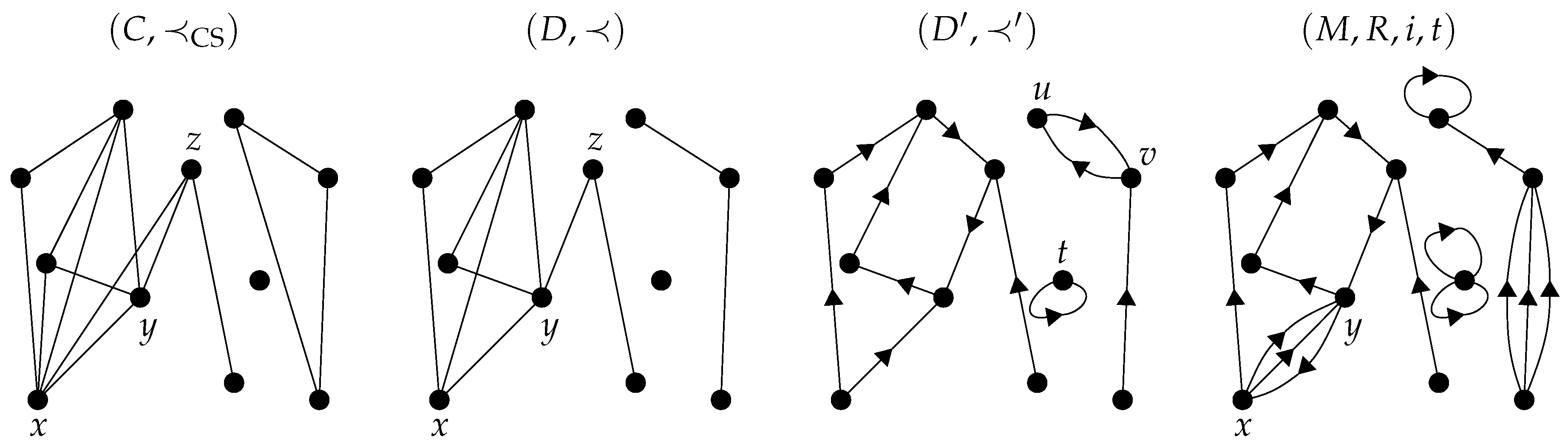
Figure 4.
Induced relation between relations and in a directed set D; global view of .

Figure 5.
Cauchy surface in a globally hyperbolic manifold X, intersected by two causal curves; maximal antichain in a directed set D, permeated by two chains.
Figure 5.
Cauchy surface in a globally hyperbolic manifold X, intersected by two causal curves; maximal antichain in a directed set D, permeated by two chains.

Figure 6.
Four co-relative histories sharing a common cobase with two elements x and y and one relation ; morphisms (transitions) representing these co-relative histories.
Figure 6.
Four co-relative histories sharing a common cobase with two elements x and y and one relation ; morphisms (transitions) representing these co-relative histories.
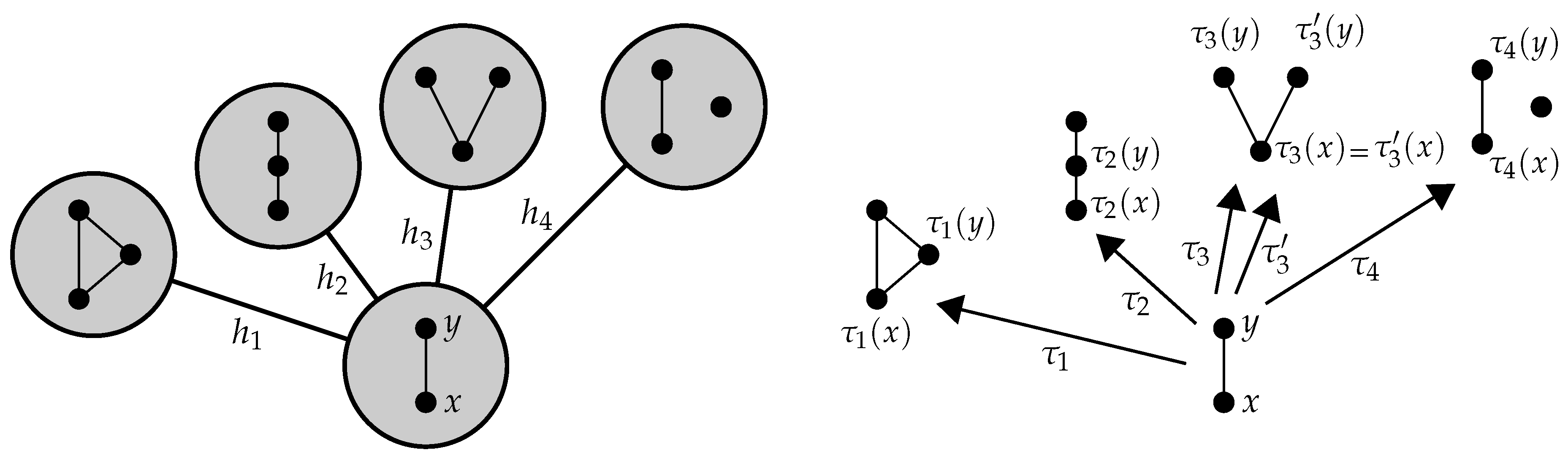
Figure 7.
Positive sequential kinematic scheme (first four generations); gray nodes show the four co-relative histories from Figure 6; thickened edges illustrate a co-relative kinematics.
Figure 7.
Positive sequential kinematic scheme (first four generations); gray nodes show the four co-relative histories from Figure 6; thickened edges illustrate a co-relative kinematics.

Figure 8.
Portion of illustrating the permeability problem; corresponding portion of showing an impermeable maximal antichain.
Figure 8.
Portion of illustrating the permeability problem; corresponding portion of showing an impermeable maximal antichain.
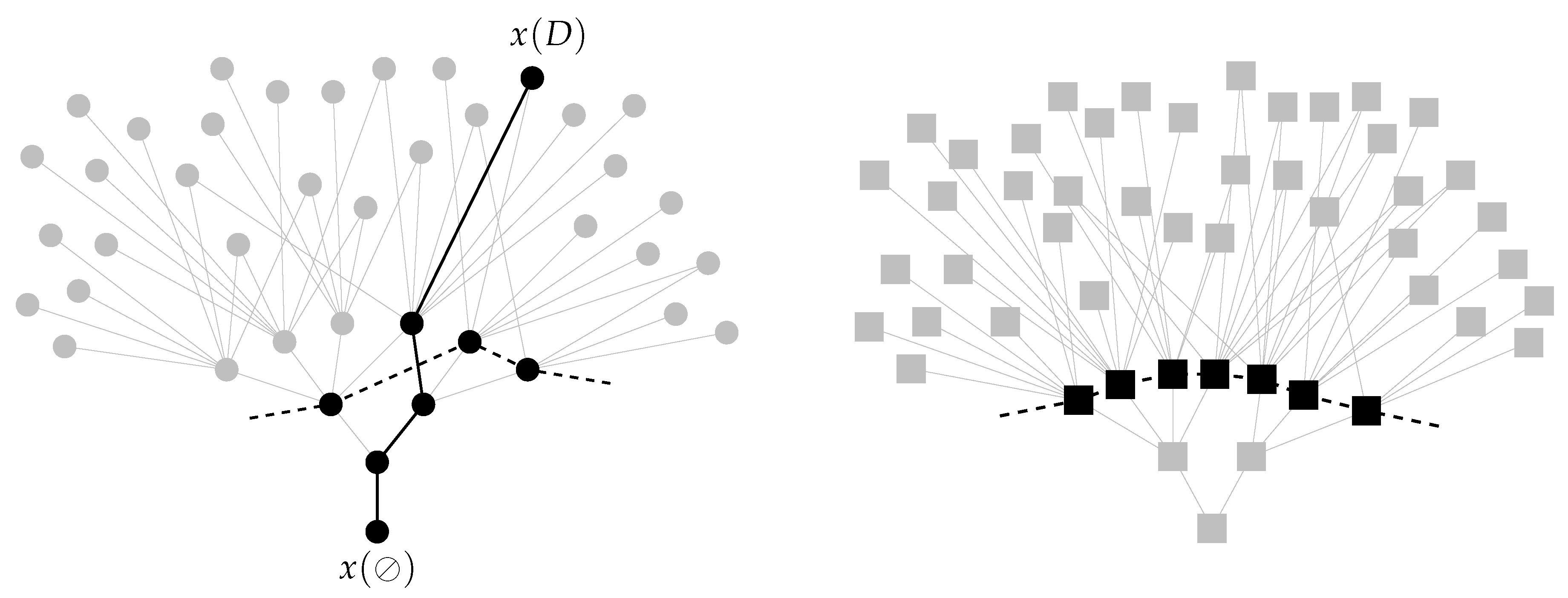
Figure 9.
Setup for deriving Equation (4): and .
Figure 9.
Setup for deriving Equation (4): and .

Figure 10.
Sequence of co-relative histories in ; terminal states indicated by dark nodes and edges; “new elements” added by each co-relative history indicated by arrows.
Figure 10.
Sequence of co-relative histories in ; terminal states indicated by dark nodes and edges; “new elements” added by each co-relative history indicated by arrows.
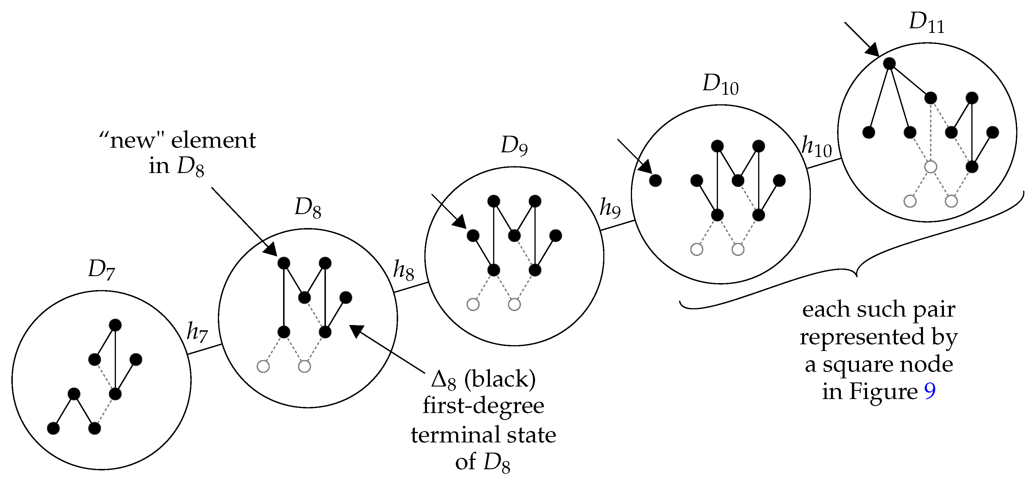
Figure 11.
Partitions of state space; conventional state spaces exhibit regions of very different sizes; state space inducing an “inverse second law of thermodynamics”.
Figure 11.
Partitions of state space; conventional state spaces exhibit regions of very different sizes; state space inducing an “inverse second law of thermodynamics”.
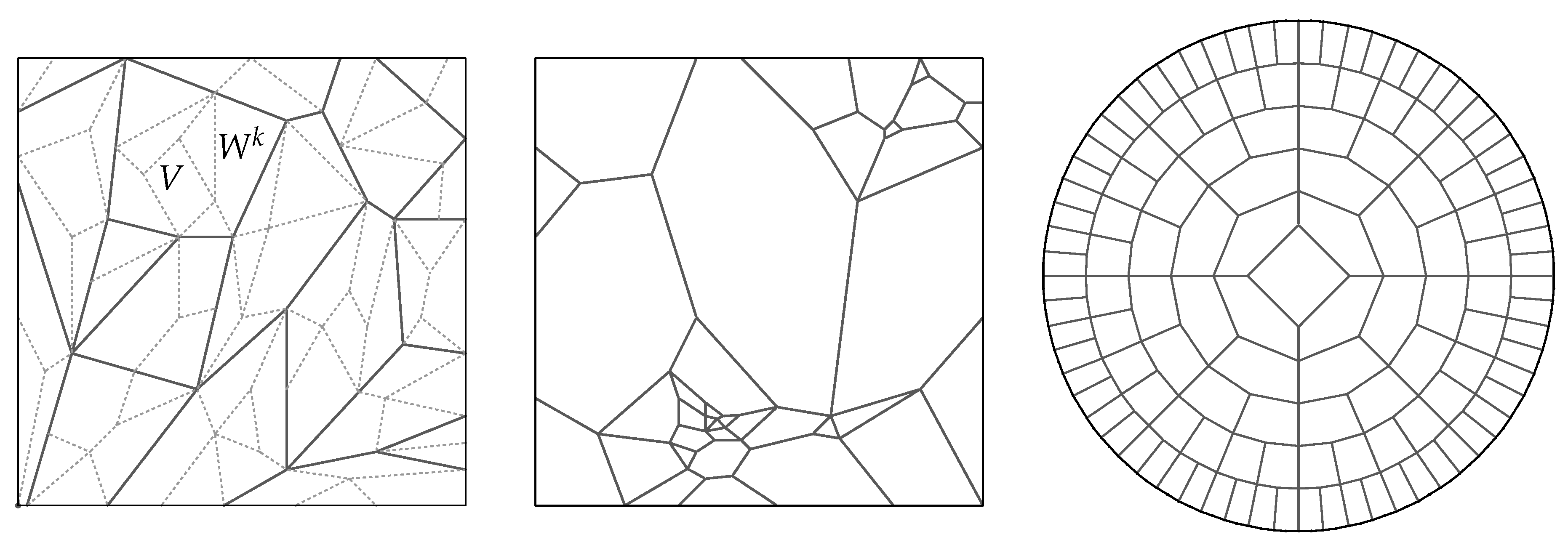
Figure 12.
A simple entropy system on the unit interval .
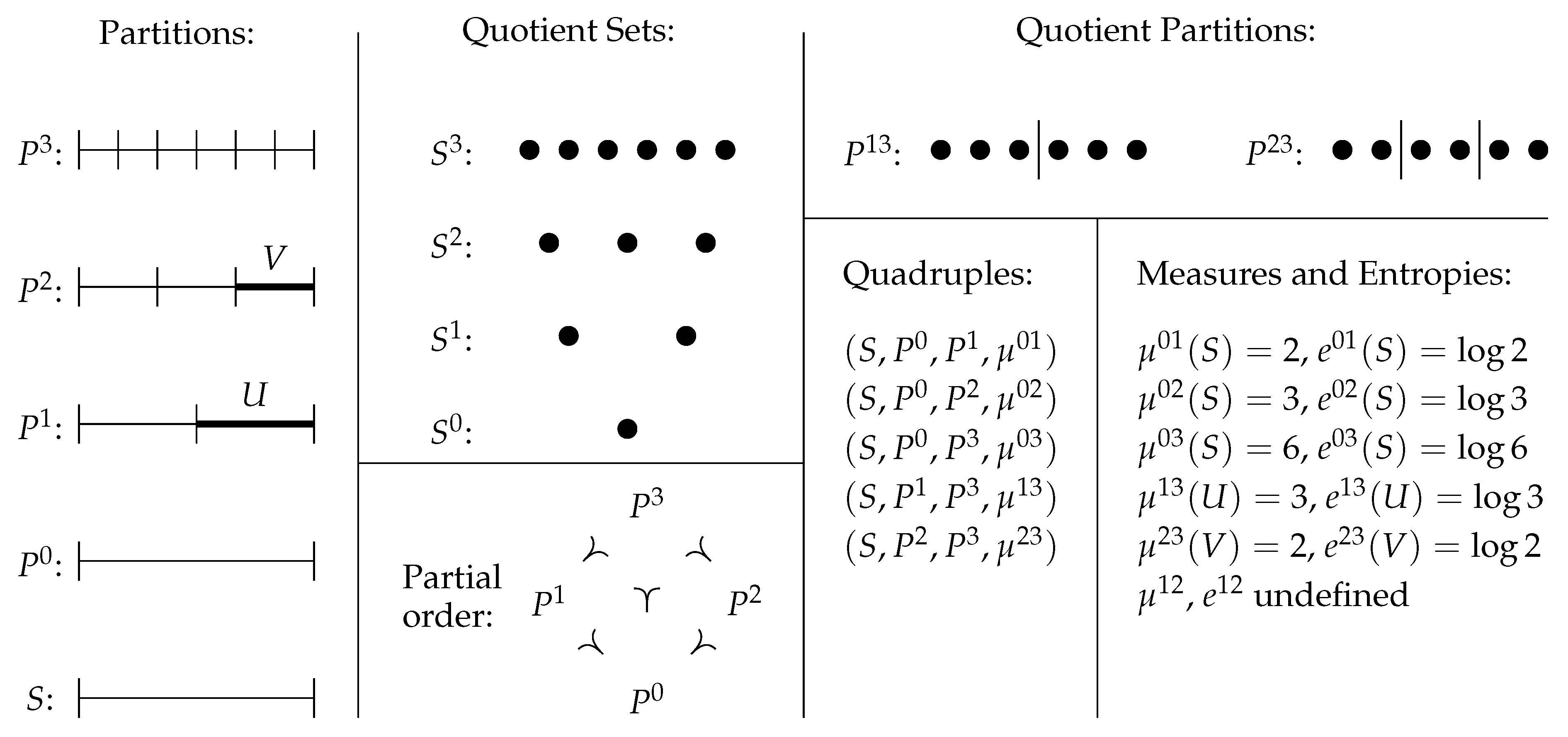
Figure 13.
Curve in state space along which entropy increases; map from a linearly ordered set into an entropy quadruple, showing no discernible second law.
Figure 13.
Curve in state space along which entropy increases; map from a linearly ordered set into an entropy quadruple, showing no discernible second law.
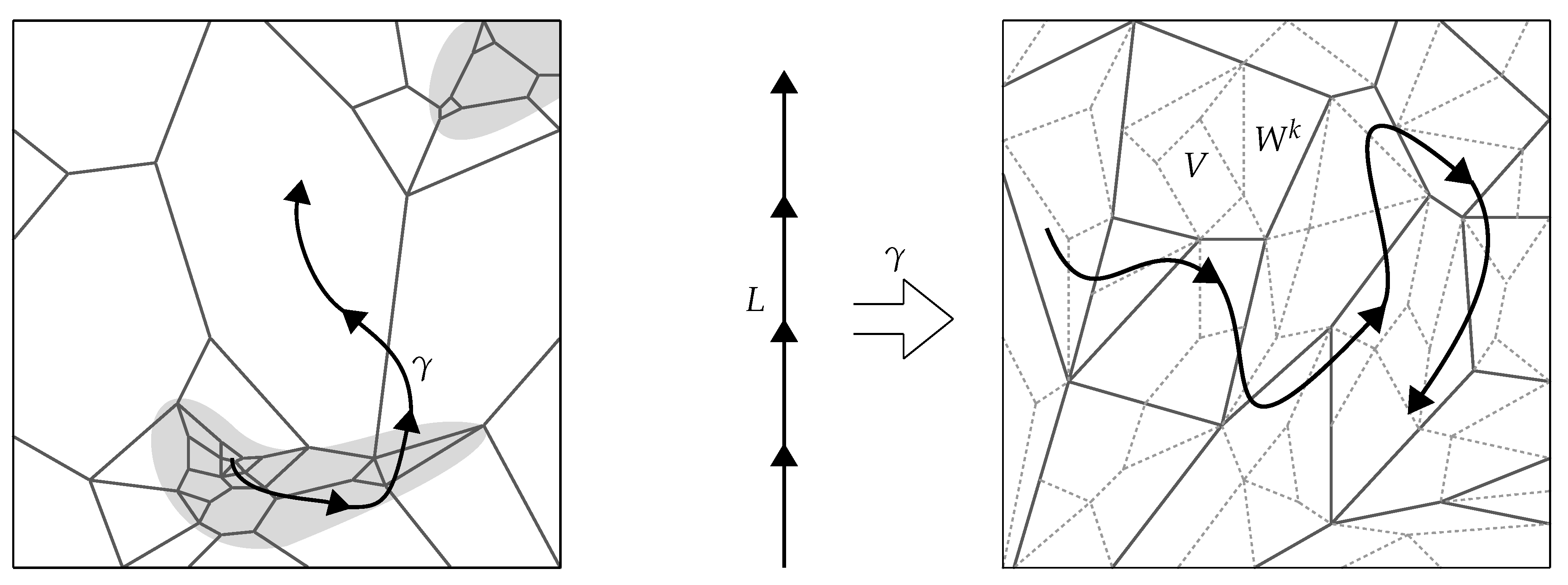
Figure 14.
History D and terminal state ; causal atomic resolution of ; superset microstate of ; labeled microstate of ; symmetry microstate of .
Figure 14.
History D and terminal state ; causal atomic resolution of ; superset microstate of ; labeled microstate of ; symmetry microstate of .
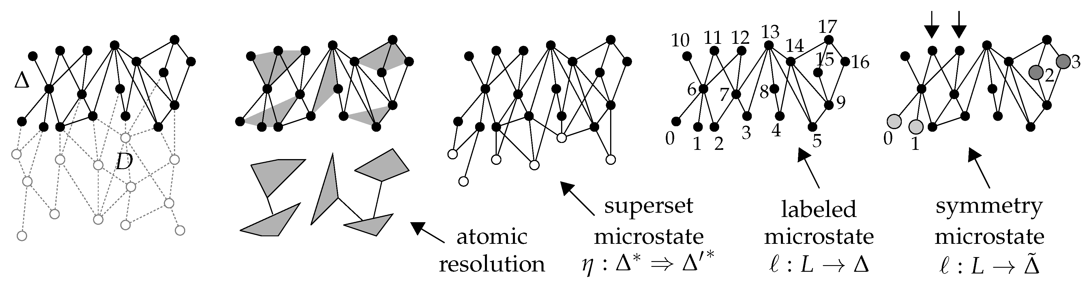
Figure 15.
22 of the 96 superset microstates of given by adding one prehistorical element.
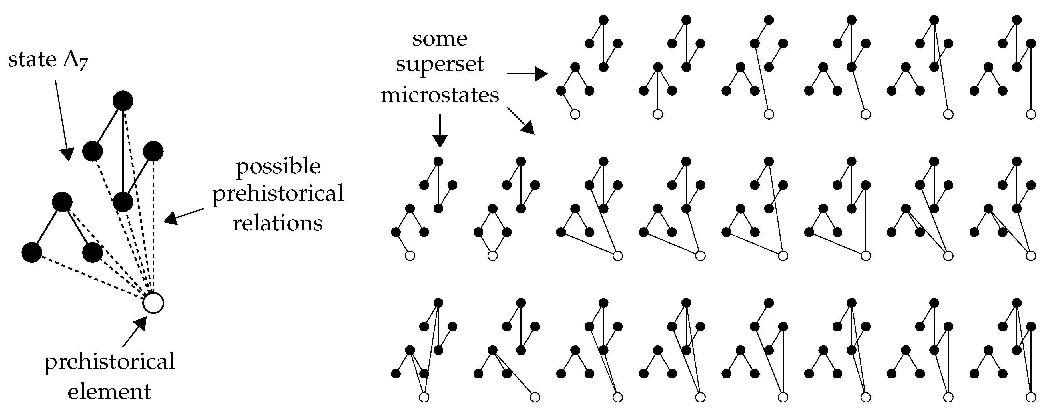
Figure 16.
McKay’s example: a superset may induce multiple microstates via pseudosimilarity.
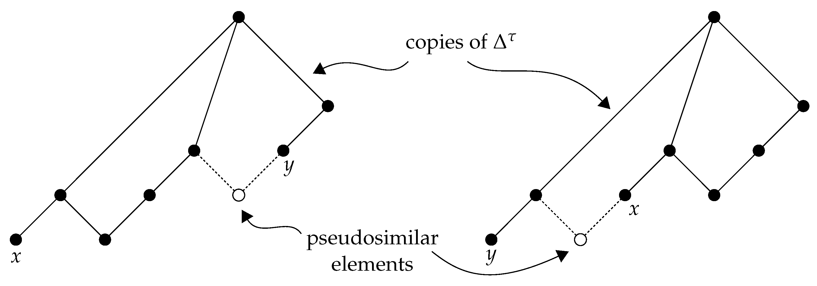
Figure 17.
Sequential growth process from Figure 10; region of through which this process moves; abstract view of the process.
Figure 17.
Sequential growth process from Figure 10; region of through which this process moves; abstract view of the process.
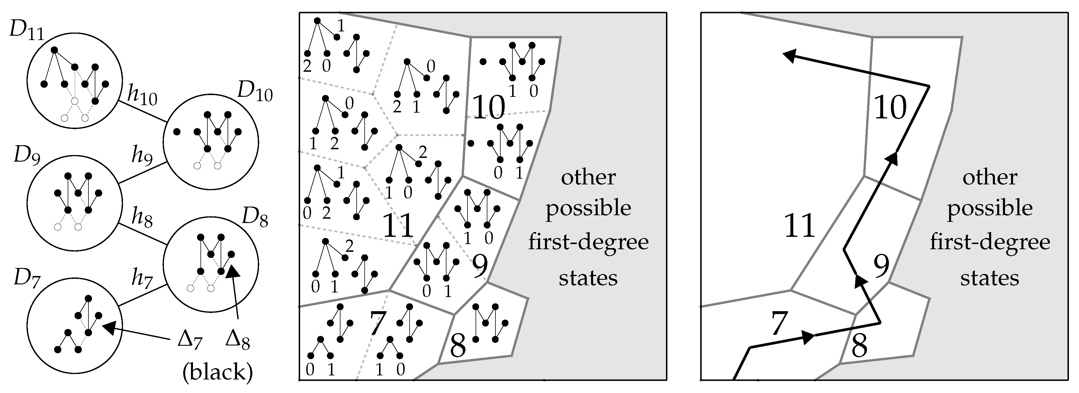
Figure 18.
Sequence of co-relative histories suggestive of gravitational collapse.
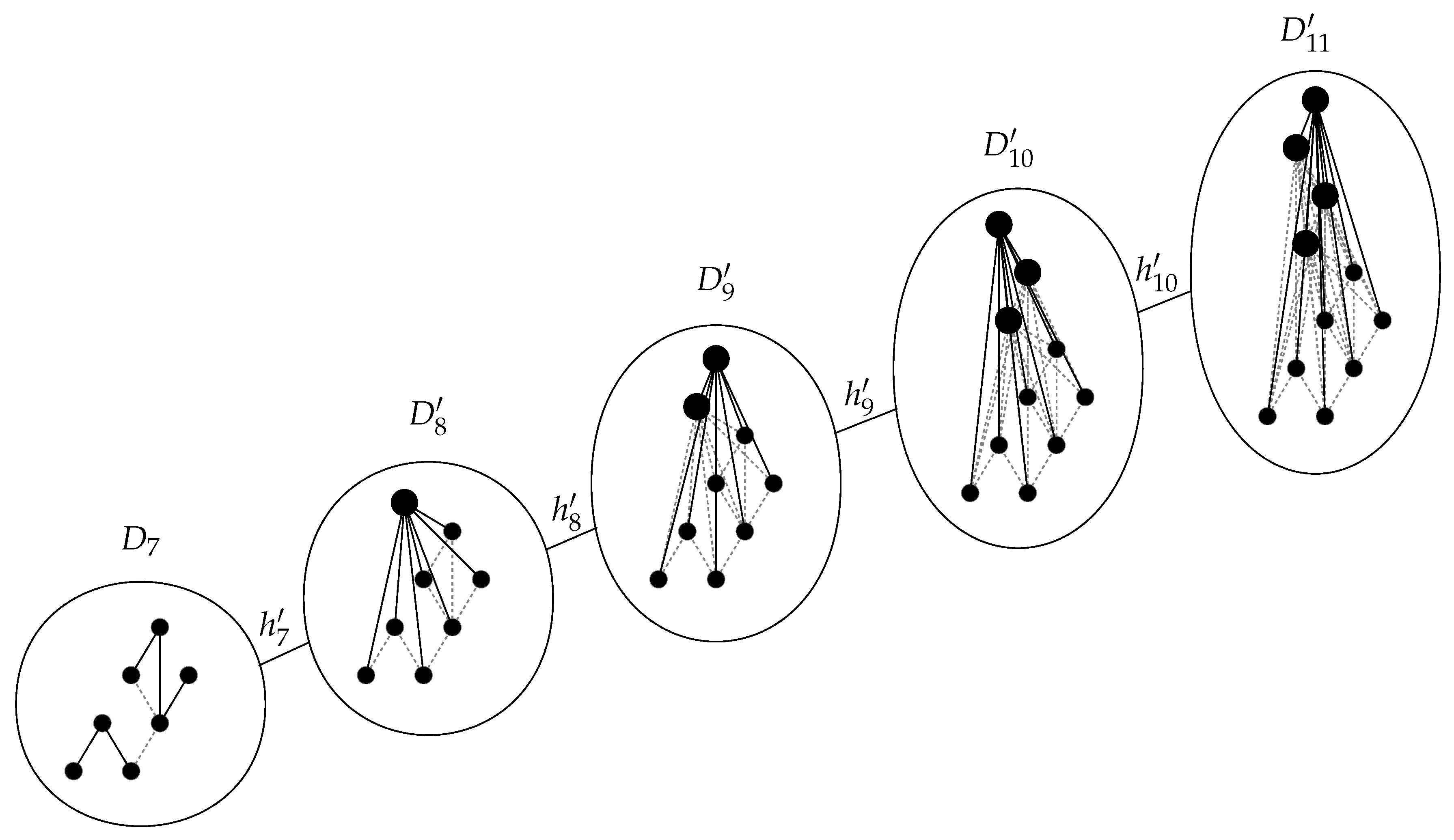
© 2017 by the author. Licensee MDPI, Basel, Switzerland. This article is an open access article distributed under the terms and conditions of the Creative Commons Attribution (CC BY) license (http://creativecommons.org/licenses/by/4.0/).
Share and Cite
MDPI and ACS Style
Dribus, B.F. Entropic Phase Maps in Discrete Quantum Gravity. Entropy 2017, 19, 322. https://doi.org/10.3390/e19070322
AMA Style
Dribus BF. Entropic Phase Maps in Discrete Quantum Gravity. Entropy. 2017; 19(7):322. https://doi.org/10.3390/e19070322
Chicago/Turabian StyleDribus, Benjamin F. 2017. "Entropic Phase Maps in Discrete Quantum Gravity" Entropy 19, no. 7: 322. https://doi.org/10.3390/e19070322
Note that from the first issue of 2016, this journal uses article numbers instead of page numbers. See further details here.