An Entropic Approach for Pair Trading

Abstract

In this paper, we derive the optimal boundary for pair trading. This boundary defines the points of entry into or exit from the market for a given stock pair. However, if the assumed model contains uncertainty, the resulting boundary could result in large losses. To avoid this, we develop a more robust strategy by accounting for the model uncertainty. To incorporate the model uncertainty, we use the relative entropy as a penalty function in the expected profit from pair trading.

1. Introduction

Pair trading is a method developed by Nunzio Tartaglia’s trading group at Morgan Stanley. This trading method is characterized by the use of a pair of stocks that have the property of mean reversion. In practice, the investor sets the position by purchasing (or short selling) a unit of one stock and short selling (or purchasing) units of another stock when the difference between these stocks diverts from the mean. The investor makes a profit by liquidating the position when the difference between the pair converges to the mean. Of course, it is also possible for an investor to take a position when the value of the pair touches the mean and to liquidate it when the value of the pair diverges sufficiently. This trading rule is the essence of pair trading.

Tartaglia’s group were hugely successful in their execution of pair trading; e.g., it is reported that they made a $50 million profit in 1987. However, the most important feature of this method is not making a big profit but stably making a profit. It is thus considered one of the most popular “market-neutral” trading methods.

The method has undergone considerable development since its introduction. Reference [1] is one of the most cited papers in this context. A good review of this context was written by [2]. Pair trading has been extended from a pair of two stocks to a more flexible portfolio showing mean reversion; e.g., statistical arbitrage [3,4]. As a first step, the pair trading was applied to the stock market. However, it can be applied to other securities. Indeed, Caporale et al. [5] apply pair trading to the foreign exchange market.

Pair trading has the appearance of being very simple. However, in practical applications of pair trading, we have two problems. First, how do we derive the mean-reverted point at which the value of the pair will converge? Second, how can we identify the entry and exit points of the trade?

The first problem is related to model risk or model uncertainty. This is caused by the misspecification of the model assumptions or the incorrect estimation of the model parameters.

Regarding the second problem, the optimal entry or exit points for pair trading are often derived by considering the optimal stopping problem (statistical analysis is also conducted to derive optimal exit or entry points [6,7]). Indeed, the solution to this problem derives an optimal boundary such that, when the value of the pair touches the boundary, it is optimal to lengthen or shorten the position of the pair. However, the second problem is strongly related to the first, because the optimal stopping problem is formulated based on parameters including the mean-reverted points derived in the first problem. Thus, any misspecification of the model results in the failure of the optimal stopping solution.

To overcome this, Ekström et al. [8] suggested that investors should identify the loss cut line and derive a strategy with regard to the optimal stopping problem that takes this line into account.

This is an intuitive and straightforward approach to overcome the problems encountered in deriving optimal stopping criteria. However, in this paper, we overcome the problems by directly addressing the misspecification of the model, because such a strategy may provide a more robust solution (similar trials have been reported by [9,10,11], although these studies did not focus on pair trading). That is, we derive the optimal strategy for pair trading in regard to the optimal stopping criteria by taking into account the model misspecification.

One candidate method of tackling the above problem is introducing fuzzy logic, which is built on the notion of fuzzy sets. The standing characteristic of the fuzzy set is the incorporation of the idea of partial membership. This feature of fuzzy sets makes it possible to discriminate elements with borderline importance that involve imprecision and uncertainty. Thus, the introduction of fuzzy logic in deriving an optimal strategy may lead to a sophisticated transaction flag, such as “strong sell (buy)”, “sell (buy)”, “weak sell (buy)” and “hold”, when the pair value touches exit or entry points (see [12] for more details on fuzzy sets and [13,14,15] on the application of fuzzy logic for finance).

Another candidate is to introduce the entropy as a penalty function for the misspecification of the model. In this paper, we focus on this. Note that the essence of the model uncertainty is that we are not sure whether the reference measure P, which is often estimated by statistical methods like maximum likelihood estimation, represents the true probability measure. Thus, we solve the optimal stopping problem by embedding the relative entropy as a penalty function.

We can see the wide applicability of entropy for finance. Indeed, entropy may be applied to risk management; e.g., Bowden [16] suggest a method of using entropy to inspect the tail risk. An entropic risk measure may signal a financial crisis [17,18,19]. As another measure related to entropy, Yang and Qiu [20] suggest the expected utility-entropy measure. Furthermore, the entropic approach with the Black–Scholes option pricing model [21] and with the estimation problem of a stochastic discount factor [22] is known to be consistent. In addition, an entropy-based approach assists time series analysis; e.g., Bekiros [23] shows application of the entropy-based approach for timescale analysis.

The introduction of the relative entropy as a penalty function is a robust approach in the sense that we construct a trading strategy based on maximizing the profit via pair trading and minimizing the relative entropy with respect to the reference measure P, even if this measure is incorrectly specified. In this paper, we describe an explicit strategy with regards to this approach. Note that, while fuzzy logic may give us information that is more sophisticated, leaving the exit or entry points as estimated by the reference measure, the penalty function based on entropy will correct the exit or entry points themselves. This is the main difference between these approaches.

This paper is organized as follows. The next section describes the model and the basic results from the optimal stopping problem for pair trading without taking into account the model uncertainty. Section 3 presents the optimal strategy for pair trading taking into account the model uncertainty and numerical examples. Section 4 is devoted to show the proof of Theorem 1. Finally, we conclude the paper with some remarks.

2. Model

The probability space is given by $(\mathsf{\Omega },\mathcal{F},\mathbb{F},P)$, where $\mathbb{F}:={\left({\mathcal{F}}_t\right)}_{t\in [0,\infty )}$. We assume that ${\mathcal{F}}_0$ is the trivial $\sigma$-field and that $\mathcal{F}$ is the $\sigma$-field generated by the union of all ${\mathcal{F}}_t,t\in [0,\infty )$.

The essence of pair trading is to use the mean-reversion of the composite process of two stock processes. As in [1], we consider an Ornstein–Uhlenbeck process ${\widehat{X}}_t$ such that

$$\begin{array}{c}\hfill d{\widehat{X}}_t=-\mu ({\widehat{X}}_t-\alpha )dt+\sigma d{W}_t,{\widehat{X}}_0=\alpha ,\end{array}$$

(1)

where $\mu ,\sigma$ are positive constants and $\alpha$ is the mean-reverted point. Further, $W_t$ is a P-Brownian motion. For simplicity, we define $X_t:={\widehat{X}}_t-\alpha$. Then, it holds that

$$\begin{array}{c}\hfill d{X}_t=-\mu X_{t}dt+\sigma d{W}_t,X_0=0.\end{array}$$

(2)

For the process $X_t$, we consider the following optimal stopping problem:

$$\begin{array}{c}\hfill v^0\left(x\right)=\underset{\tau \in \mathcal{T}}{sup}{\mathbb{E}}_x\left[e^{-\rho \tau }{X}_{\tau }\right],\end{array}$$

(3)

where $\mathcal{T}$ is a set of all stopping times of W and $\rho$ is the discount rate. We also assume that $\mathbb{E}\tau <\infty$ for all $\tau \in \mathcal{T}$. The solution of problem (3) implies a trading strategy in which we short pair X when X attains the highest value specified by the solution of (3) and liquidate this when X attains a value of zero. The other implied strategy is that we take a long position on pair X when X is zero and liquidate this when X reaches its highest point.

Let us consider the condition that we are now at time t, and at this time $x=X_t$. Then, our problem is to solve $e^{-\rho t}{v}^0\left(x\right)$. According to Itô’s lemma, it follows that

$$\begin{array}{cc}\hfill d\left(e^{-\rho t}{v}^0\left(x\right)\right)& =-\rho e^{-\rho t}{v}^0\left(x\right)dt+\frac{\partial e^{-\rho t}{v}^0\left(x\right)}{\partial x}d{X}_t+\frac{1}{2}\frac{\partial e^{-\rho t}{v}^0\left(x\right)}{\partial x^2}d{\langle X\rangle }_t\hfill \\ & =\left(-\rho e^{-\rho t}{v}^0\left(x\right)-e^{-\rho t}\mu x{v}_x^0\left(x\right)+\frac{1}{2}{e}^{-\rho t}{\sigma }^2{v}_{xx}^0\left(x\right)\right)dt+e^{-\rho t}\sigma d{W}_t.\hfill \end{array}$$

Theorems 2.4 and 2.7 of [24] imply that the optimal solution of problem (3) requires the existence of a boundary b such that $v^0\left(b\right)=b$ if $x\ge b$, otherwise $v^0\left(x\right)>x$ and the martingale property; i.e.,

$$\begin{array}{c}\hfill \frac{1}{2}{\sigma }^2{v}_{xx}^0\left(x\right)-\mu x{v}_x^0\left(x\right)-\rho v^0\left(x\right)=0.\end{array}$$

Further, according to Theorem 9.5 of [24], the smooth fit condition holds; i.e., $v_x^0\left(b\right)=1$ for $x=b$.

Summarizing the above, we have to solve the following free-boundary problem:

$$\begin{array}{c}\hfill -\mu x{v}_x^0+\frac{1}{2}{\sigma }^2{v}_{xx}^0=\rho v^0\mathrm{for}x<b,\end{array}$$

(4)

$$\begin{array}{c}\hfill v^0\left(b\right)=b\mathrm{for}x\ge b,\end{array}$$

(5)

$$\begin{array}{c}\hfill v_x^0\left(b\right)=1\mathrm{for}x=b.\end{array}$$

(6)

From these expressions, we can easily derive

$$\begin{array}{c}\hfill v^0\left(x\right)=\frac{\sigma }{\sqrt{2\mu }}\frac{{\int }_0^{\infty }{u}^{\frac{\rho }{\mu }-1}{e}^{\frac{\sqrt{2\mu }}{\sigma }ux-\frac{u^2}{2}}du}{{\int }_0^{\infty }{u}^{\frac{\rho }{\mu }}{e}^{\frac{\sqrt{2\mu }}{\sigma }ub-\frac{u^2}{2}}du}.\end{array}$$

Further, the boundary $b^{*}$ satisfies the following:

$$\begin{array}{c}\hfill \frac{\sigma }{\sqrt{2\mu }}\frac{{\int }_0^{\infty }{u}^{\frac{\rho }{\mu }-1}{e}^{\frac{\sqrt{2\mu }}{\sigma }u{b}^{*}-\frac{u^2}{2}}du}{{\int }_0^{\infty }{u}^{\frac{\rho }{\mu }}{e}^{\frac{\sqrt{2\mu }}{\sigma }u{b}^{*}-\frac{u^2}{2}}du}=b^{*}.\end{array}$$

(7)

In the following section, we derive the optimal boundary when the model uncertainty is taken into account.

3. Main Results

The essence of the model uncertainty is that we are not sure whether the reference measure P represents the true probability measure. We use a class $\mathcal{Q}$ of probability measures on $(\mathsf{\Omega },\mathcal{F})$. Then, the most intuitive way to derive the multiple-prior expected optimal reward is given by

$$\begin{array}{c}\hfill \underset{\tau \in \mathcal{T}}{sup}\underset{Q\in \mathcal{Q}}{inf}{\mathbb{E}}_x^Q\left[e^{-\rho (\tau -t)}{X}_{\tau }\right].\end{array}$$

(8)

This is called the maxmin expected utility, and is often used to derive robust strategies. However, the strategy given by this approach often implies that the investor should not participate in the market. Although robust, this strategy is meaningless for investors who wish to make a profit by entering the market.

Thus, we consider a more flexible trading strategy, i.e., we consider the following optimal stopping problem conditioned on $x=X_t$ at time t:

$$\begin{array}{c}\hfill v(t,x):=\underset{\tau \in \mathcal{T}}{sup}{\mathbb{E}}_x^Q\left[e^{-\rho (\tau -t)}{X}_{\tau }\right],\end{array}$$

(9)

where Q is the solution to the following:

$$\begin{array}{c}\hfill \underset{Q\in \mathcal{Q}}{inf}\left\{{\mathbb{E}}_x^Q\left[e^{-\rho (\tau -t)}{X}_{\tau }\right]+\lambda e^{-\rho (\tau -t)}{H}_x\left[Q\right|P]\right\}.\end{array}$$

(10)

Here, $\lambda$ is a positive constant and $H(·)$ is the relative entropy defined by

$$\begin{array}{c}\hfill H_x\left(Q\right|P):=\left\{\begin{array}{cc}{\mathbb{E}}_x^Q\left[ln\left(\frac{dQ}{dP}\right)\right],\hfill & Q\in \mathcal{Q}\hfill \\ \infty ,\hfill & \mathrm{otherwise}\hfill \end{array}\right.\end{array}$$

(11)

The constant $\lambda$ reflects how accurate the agent believes the reference measure P to be, i.e., when $\lambda \uparrow \infty$, the agent has complete trust in the reference measure P, whereas when $\lambda \downarrow 0$, the agent has no confidence in P. Further, we assume the optimal boundary $b\left(t\right)$ for (9) coincides with $b^{*}$ at $t=0$; i.e., $b\left(0\right)=b^{*}$.

Theorem 1.

For $t\in [0,\infty )$, the optimal boundary $b\left(t\right)$ for (9) is given by

$$\begin{array}{cc}\hfill {\displaystyle ln}\left(b\left(t\right)\right)+\frac{1}{{\sigma }^2}\frac{\rho }{\mu -\rho }& {(g\left(t\right)-b\left(t\right))}^2\hfill \\ & =ln{b}^{*}+\frac{1}{{\sigma }^2}\frac{\rho }{\mu -\rho }{\left(b^{*}\right)}^2,\hfill \end{array}$$

where $g\left(t\right)=-\frac{{\sigma }^2}{\lambda }t{e}^{-\mu t}$.

Theorem 1 implies a strategy in which investors holding pair $X_t$ should liquidate their position when $X_t$ touches $b\left(t\right)$, while those not holding $X_t$ should short the position when X touches $b\left(t\right)$ and liquidate it when it reverts to the mean 0.

Numerical Example

Finally, we present a numerical example using market data of stocks listed on the Tokyo Stock Exchange. We choose 20 names of stocks with relatively low PERs (Price Earnings Ratio) around 1 to 5, noting that the average PER of stocks on the Tokyo Stock Exchange is about 15; i.e., Fullcast Holdings Co., Ltd. (code: 4848), Daiichi Commodities Co., Ltd. (8746), Fuji Oil Co., Ltd. (5017), FIDEA Holdings Co., Ltd. (8713), Yoshicon Co., Ltd. (5280), PADO Corporation (4833), Sado Steam Ship Co., Ltd. (9176), Joban Kaihatsu Co., Ltd. (1782), Meiwa Estate Company Limited (8869), Oi Electric Co., Ltd. (6822), Takata Corporation (7312), Toei Reefer Line Ltd. (9133), Nihon House Holdings Co., Ltd. (1873), Sanei Architecture Planning Co., Ltd. (3228), Shinhoku Steel Corporation (5542), Daiko Denshi Tsushin Ltd. (8023), Shinnihon Corporation (1879), Asahi Industries Co., Ltd. (5456), Seiwa Electric MFG. Co., Ltd. (6748), and Daisue Construction Co., Ltd. (1814).

We sampled historical data of these names from 26 March 2015 to 25 May 2015 and applied the Phillips–Ouliaris cointegration test with a p-value 0.05. We then found six pairs of cointegration from 190 ($=20!/2!18!$) pairs; i.e., (Daiichi Commodities Co., Ltd. (8746), Asahi Industries Co., Ltd. (5456)), (Fuji Oil Co., Ltd. (5017), Sado Steam Ship Co., Ltd. (9176)), (Fuji Oil Co., Ltd. (5017), Takata Corporation (7312)), (PADO Corporation (4833), Oi Electric Co., Ltd. (6822)), (PADO Corporation (4833), Seiwa Electric MFG. Co., Ltd. (6748)), and (Sado Steam Ship Co., Ltd. (9176), Daiko Denshi Tsushin Ltd (8023)).

Having found the pairs, we can estimate parameters of Ornstein–Uhlenbeck processes, $\mu ,\alpha$, and $\sigma$, via maximum likelihood estimation; e.g., the parameter of the pair value of Daiichi Commodities Co., Ltd. (8746) and Asahi Industries Co., Ltd. (5456) is given by

$$\begin{array}{c}\hfill \mu =0.99,\sigma =5.19,\alpha =231.73.\end{array}$$

To calculate the optimal boundary, we further need parameters $\rho$ and $\lambda$. Here we set $\rho =0.004$, according to the Monthly Report of the Bank of Japan issued in May 2015, where it was reported that yields on 10-year government bonds were moving in the range of 0.40–0.45 percent.

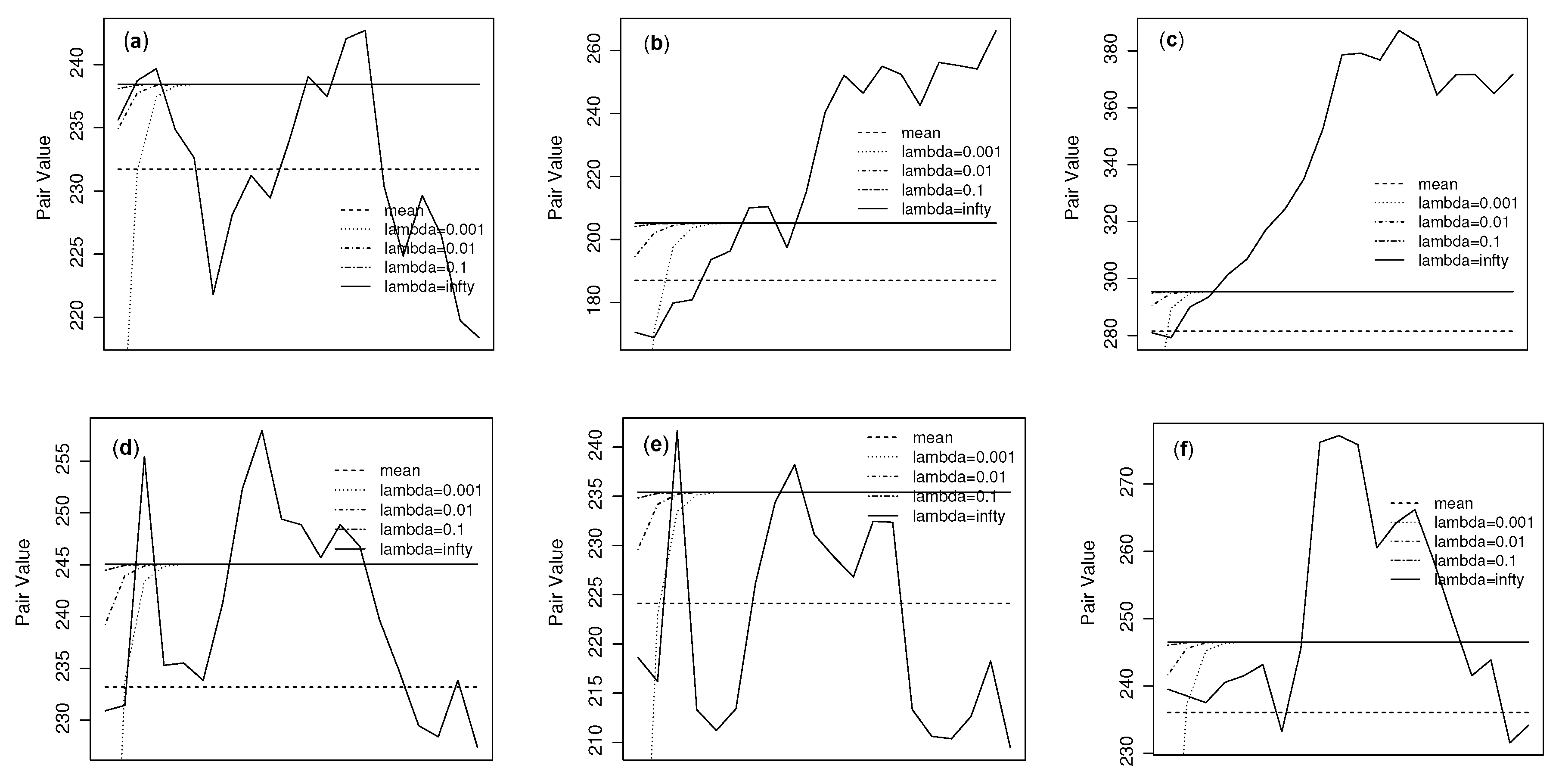
The parameter $\lambda$ depends on the investors’ trustfulness for the model. Low $\lambda$ implies low confidence while high $\lambda$ implies high confidence. Here, we consider four cases; i.e., $\lambda =0.001,0.01,0.1$ and $+\infty$. Note that the case $\lambda =+\infty$ is consistent with the case of the boundary $b^{*}$. Using these parameters, we calculate boundaries $b\left(t\right)$ for $\lambda =0.001,0.01,0.1,+\infty$ and show them in Figure 1 together with pair values of stocks from 25 May 2015 to 26 June 2015 that are outside the sample. The figure reveals that the boundary $b\left(t\right)$ with finite $\lambda$ converges to $b\left(t\right)$ with infinite $\lambda$; i.e., to $b^{*}$. Furthermore, the distance from $b\left(t\right)$ to $b^{*}$ increases as $\lambda$ decreases. This is consistent with the theory.

Furthermore, we consider the performance of our pair trading strategy using real market data. The trading policy is set as follows. The position is set when the pair value touches either the boundary $b\left(t\right)$ or the mean-reverted point $\alpha$. If the position is set for the case that the pair value touches $b\left(t\right)$, the position is liquidated when the pair value touches the mean-reverted point, and vice versa. After the liquidation, the next position is set when the pair value touches either $b\left(t\right)$ or $\alpha$ and this position is liquidated by the same rule, and so forth. According to this trading policy, we simulate the rate of return for pair trading, using a sample from 25 May 2015 to 2 September 2015. The rate of return of this trading policy is presented in

Table 1. The rate of return for different $\lambda$. Pair 1 is Daiichi Commodities Co., Ltd. (8746) and Asahi Industries Co., Ltd. (5456); Pair 2 is Fuji Oil Co., Ltd. (5017) and Sado Steam Ship Co., Ltd. (9176); Pair 3 is Fuji Oil Co., Ltd. (5017) and Takata Corporation (7312); Pair 4 is PADO Corporation (4833) and Oi Electric Co., Ltd. (6822); Pair 5 is PADO Corporation (4833) and Seiwa Electric MFG. Co., Ltd. (6748); Pair 6 is Sado Steam Ship Co., Ltd. (9176), Daiko Denshi Tsushin Ltd. (8023).

	$\mathit{\lambda }=0.001$	$\mathit{\lambda }=0.01$	$\mathit{\lambda }=0.1$	$\mathit{\lambda }=+\mathbf{\infty }$
Pair 1	0.152	0.152	0.165	0.165
Pair 2	0.321	0.170	0.170	0.170
Pair 3	0.071	0.028	0.028	0.028
Pair 4	0.189	0.076	0.076	0.076
Pair 5	0.097	0.088	0.088	0.088
Pair 6	0.093	0.133	0.133	0.133

.

As [2,3] pointed out, an important obstacle for the pair trading to make a profit is the transaction fee. One transaction of pair trading requires transaction fees to be charged twice, owing to the requirement of two stocks. Furthermore, there may be frequent transactions for pair trading if the investor often determines profits for the movement of the pair value. We thus discounted the loss due to the transaction fee from the rate of return. The results given in Table 1 are these discounted returns. Although the transaction fee depends on the market maker, 0.1% for one transaction may be used in the Japanese market. We discounted 0.2% for one transaction because our trading policy is based on pair trading.

For the evaluation of the above result, we compare the result with the rate of return of another trading policy. We here consider the buy-and-hold strategy. Because all stocks used in this numerical example have small PERs, they may be good candidates for the buy-and-hold strategy.

Similarly for the trading policy of pair trading discussed above, we used the sample ranging from 25 May 2015 to 2 September 2015. The buy-and-hold strategy requires only the buying of a stock on 25 May 2015 and the liquidation of the stock on 2 September 2015. For this simple strategy, the rate of return is summarized in

Table 2. Return of buy-and-hold strategy for low PER stocks.

Names	Return
Fullcast Holdings Co., Ltd. (code: 4848)	0.099
Daiichi Commodities Co., Ltd. (8746)	−0.113
Fuji Oil Co., Ltd. (5017)	−0.091
FIDEA Holdings Co., Ltd. (8713)	−0.125
Yoshicon Co., Ltd. (5280)	0.016
PADO Corporation (4833)	−0.157
Sado Steam Ship Co., Ltd. (9176)	−0.016
Joban Kaihatsu Co., Ltd. (1782)	−0.047
Meiwa Estate Company Limited (8869)	−0.026
Oi Electric Co., Ltd. (6822)	−0.059
Takata Corporation (7312)	−0.034
Toei Reefer Line Ltd. (9133)	−0.147
Nihon House Holdings Co., Ltd. (1873)	−0.076
Sanei Architecture Planning Co., Ltd. (3228)	0.521
Shinhoku Steel Corporation (5542)	−0.275
Daiko Denshi Tsushin Ltd. (8023)	−0.226
Shinnihon Corporation (1879)	0.193
Asahi Industries Co., Ltd. (5456)	−0.121
Seiwa Electric MFG. Co., Ltd. (6748)	−0.050
Daisue Construction Co., Ltd. (1814)	−0.129

.

Except for a few stocks, almost all stocks make a loss for this strategy, at least in the term considered. We note that even if we choose the group of stocks using criteria other than the PER and the buy-and-hold strategy makes a big profit, it may not be stable. Table 1 gives the stability of pair trading. This is why we suggest the trading strategy of pair trading while taking model uncertainty into account.

4. Proof of Theorem 1

Proof of Theorem 1.

For the argument of (10), it holds

$$\begin{array}{cc}\hfill \int \left(e^{-\rho (\tau -t)}{X}_{\tau }+\lambda e^{-\rho (\tau -t)}ln\left(\frac{dQ}{dP}\right)\right)dQ& =\lambda e^{-\rho (\tau -t)}\int ln\left(e^{X_{\tau }/\lambda }\frac{dQ}{dP}\right)dQ.\hfill \end{array}$$

Noting that the relative entropy $H\left[Q\right|P]$ is minimized when $Q=P$, the above implies that the optimality of (10) is attained by the following (the more detailed process is supported by [25,26]):

$$\begin{array}{c}\hfill \frac{dQ}{dP}{|}_{{\mathcal{F}}_t}=\frac{e^{-X_t/\lambda }}{{\mathbb{E}}_x\left[e^{-X_t/\lambda }\right]}.\end{array}$$

(12)

Since $d{X}_t=-\mu X_{t}dt+\sigma d{W}_t$, $X_t=e^{-\mu t}\left(X_0+{\int }_0^t\sigma e^{\mu s}d{W}_s\right)$. Hence,

$$\begin{array}{cc}\hfill \frac{dQ}{dP}{|}_{{\mathcal{F}}_t}=& \frac{e^{-X_t/\lambda }}{{\mathbb{E}}_x\left[e^{-X_t/\lambda }\right]}=\frac{e^{-\frac{1}{\lambda }{e}^{-\mu t}\left(X_0+{\int }_0^t\sigma e^{\mu s}d{W}_s\right)}}{{\mathbb{E}}_x\left[e^{-\frac{1}{\lambda }{e}^{-\mu t}\left(X_0+{\int }_0^t\sigma e^{\mu s}d{W}_s\right)}\right]}\hfill \\ \hfill =& \frac{e^{-\frac{1}{\lambda }{\int }_0^t\sigma e^{\mu (s-t)}d{W}_s}}{{\mathbb{E}}_x\left[e^{-\frac{1}{\lambda }{\int }_0^t\sigma e^{\mu (s-t)}d{W}_s}\right]}.\hfill \end{array}$$

From this and Girsanov, Cameron and Martin theorem, Q-Brownian motion $W^{*}$ is given by

$$\begin{array}{cc}\hfill W_t^{*}& =W_t+\frac{\sigma }{\lambda \mu }\left(1-e^{-\mu t}\right).\hfill \end{array}$$

Then, the dynamics of X is given by

$$\begin{array}{cc}\hfill d{X}_t& =-\left(\mu X_t+\frac{{\sigma }^2}{\lambda }{e}^{-\mu t}\right)dt+\sigma d{W}_t^{*}.\hfill \end{array}$$

(13)

Set the problem conditioned on $x=X_t$:

$$\begin{array}{c}\hfill v^1(t,x)=\underset{\tau \in \mathcal{T}}{sup}{\mathbb{E}}_x^Q\left[e^{-\rho \tau }{X}_{\tau }\right]\end{array}$$

Further, when $t\uparrow \infty$, the structure of X in (13) is same as in (2). Hence, it follows ${lim}_{t\uparrow \infty }{v}^1(t,x)=v^0\left(x\right)$.

We apply Itô’s lemma for $v(t,x)=e^{-\rho t}{v}^1(t,x)$ as follows:

$$\begin{array}{cc}\hfill d& \left(e^{-\rho t}{v}^1(t,x)\right)=-\rho e^{-\rho t}{v}^{1}dt+e^{-\rho t}{v}_t^{1}dt+e^{-\rho t}{v}_z^{1}d{X}_t+\frac{1}{2}{e}^{-\rho t}{v}_{xx}^{1}d{\langle X\rangle }_t\hfill \\ & =-\rho e^{-\rho t}{v}^{1}dt+e^{-\rho t}{v}_t^{1}dt+e^{-\rho t}{v}_x^1\left(-\left(\mu X_t+\frac{{\sigma }^2}{\lambda }{e}^{-\mu t}\right)dt+\sigma d{W}_t^{*}\right)+\frac{1}{2}{e}^{-\rho t}{v}_{xx}^1{\sigma }^{2}dt\hfill \\ & =\left(-\rho e^{-\rho t}{v}^1+e^{-\rho t}{v}_t^1-e^{-\rho t}{v}_x^1\left(\mu X_t+\frac{{\sigma }^2}{\lambda }{e}^{-\mu t}\right)+\frac{1}{2}{e}^{-\rho t}{v}_{xx}^1{\sigma }^2\right)dt+e^{-\rho t}{v}_x^1\sigma d{W}_t^{*}.\hfill \end{array}$$

According to Theorems 2.4 and 2.7 of [24], the optimal solution of problem (3) requires the existence of a boundary $b\left(t\right)$ such that $v^1(t,b\left(t\right))=b\left(t\right)$ if $x\ge b\left(t\right)$, otherwise $v^1(t,x)>x$ and the martingale property; i.e.,

$$\begin{array}{c}\hfill -\rho v^1+v_t^1-\left(\mu X_t+\frac{{\sigma }^2}{\lambda }{e}^{-\mu t}\right)v_x^1+\frac{1}{2}{\sigma }^2{v}_{xx}^1=0.\end{array}$$

Further, Theorem 9.5 of [24] implies that $v_x^1(t,b\left(t\right))=b^{\prime }\left(t\right)$ for $x=b\left(t\right)$.

Therefore, our free boundary problem is deduced as follows:

$$\begin{array}{c}\hfill -\rho v^1+v_t^1-\left(\mu X_t+\frac{{\sigma }^2}{\lambda }{e}^{-\mu t}\right)v_x^1+\frac{1}{2}{\sigma }^2{v}_{xx}^1=0\mathrm{for}x<b\left(t\right),\end{array}$$

(14)

$$\begin{array}{c}\hfill v^1(t,b\left(t\right))=b\left(t\right)\mathrm{for}x\ge b\left(t\right),\end{array}$$

(15)

$$\begin{array}{c}\hfill \partial v^1(t,b\left(t\right))/\partial t=b^{\prime }\left(t\right)\mathrm{for}x=b\left(t\right).\end{array}$$

(16)

Let $v^1(t,x)=c_1{\int }_0^{\infty }{u}^{\frac{\rho }{\mu }-1}{e}^{\frac{\sqrt{2\mu }}{\sigma }\left(x-g\left(t\right)\right)u-\frac{u^2}{2}}du+c_2$, where $g\left(t\right)=-\frac{{\sigma }^2}{\lambda }t{e}^{-\mu t}+c_3{e}^{-\mu t}$. By applying this for (14), it follows $c_2=0$. Note that ${lim}_{t\to \infty }{v}^1(t,x)=c_1{\int }_0^{\infty }{u}^{\frac{\rho }{\mu }-1}{e}^{\frac{\sqrt{2\mu }}{\sigma }xu-\frac{u^2}{2}}du$, where we used ${lim}_{t\to \infty }g\left(t\right)=0$. Then, it holds

$$\begin{array}{c}\hfill c_1{\int }_0^{\infty }{u}^{\frac{\rho }{\mu }-1}{e}^{\frac{\sqrt{2\mu }}{\sigma }xu-\frac{u^2}{2}}du=v^0\left(x\right)=\frac{\sigma }{\sqrt{2\mu }}\frac{{\int }_0^{\infty }{u}^{\frac{\rho }{\mu }-1}{e}^{\frac{\sqrt{2\mu }}{\sigma }ux-\frac{u^2}{2}}du}{{\int }_0^{\infty }{u}^{\frac{\rho }{\mu }}{e}^{\frac{\sqrt{2\mu }}{\sigma }u{b}^{*}-\frac{u^2}{2}}du}.\end{array}$$

This implies that $c_1=\frac{\sigma }{\sqrt{2\mu }}\frac{1}{{\int }_0^{\infty }{u}^{\frac{\rho }{\mu }}{e}^{\frac{\sqrt{2\mu }}{\sigma }u{b}^{*}-\frac{u^2}{2}}du}$. Finally, we attain the form of $v^1(t,x)$ as follows:

$$\begin{array}{c}\hfill v^1(t,x)=\frac{\sigma }{\sqrt{2\mu }}\frac{{\int }_0^{\infty }{u}^{\frac{\rho }{\mu }-1}{e}^{\frac{\sqrt{2\mu }}{\sigma }\left(x-g\left(t\right)\right)u-\frac{u^2}{2}}du}{{\int }_0^{\infty }{u}^{\frac{\rho }{\mu }}{e}^{\frac{\sqrt{2\mu }}{\sigma }u{b}^{*}-\frac{u^2}{2}}du}.\end{array}$$

As regard with (15),

$$\begin{array}{c}\hfill v^1(t,b\left(t\right))=\frac{\sigma }{\sqrt{2\mu }}\frac{{\int }_0^{\infty }{u}^{\frac{\rho }{\mu }-1}{e}^{\frac{\sqrt{2\mu }}{\sigma }\left(b\left(t\right)-g\left(t\right)\right)u-\frac{u^2}{2}}du}{{\int }_0^{\infty }{u}^{\frac{\rho }{\mu }}{e}^{\frac{\sqrt{2\mu }}{\sigma }u{b}^{*}-\frac{u^2}{2}}du}=b\left(t\right).\end{array}$$

(17)

Further, according to (16),

$$\begin{array}{c}{\displaystyle v_t^1(t,b\left(t\right))+v_x^1(t,b\left(t\right))b^{\prime }\left(t\right)}\hfill \\ =-g^{\prime }\left(t\right)\frac{{\int }_0^{\infty }{u}^{\frac{\rho }{\mu }}{e}^{\frac{\sqrt{2\mu }}{\sigma }u\left(b\left(t\right)-g\left(t\right)\right)-\frac{u^2}{2}}du}{{\int }_0^{\infty }{u}^{\frac{\rho }{\mu }}{e}^{\frac{\sqrt{2\mu }}{\sigma }u{b}^{*}-\frac{u^2}{2}}du}+\frac{{\int }_0^{\infty }{u}^{\frac{\rho }{\mu }}{e}^{\frac{\sqrt{2\mu }}{\sigma }u\left(b\left(t\right)-g\left(t\right)\right)-\frac{u^2}{2}}du}{{\int }_0^{\infty }{u}^{\frac{\rho }{\mu }}{e}^{\frac{\sqrt{2\mu }}{\sigma }u{b}^{*}-\frac{u^2}{2}}du}{b}^{\prime }\left(t\right)=b^{\prime }\left(t\right).\hfill \end{array}$$

That is,

$$\begin{array}{cc}\hfill b^{\prime }\left(t\right)& =(b^{\prime }\left(t\right)-g^{\prime }\left(t\right))\frac{{\int }_0^{\infty }{u}^{\frac{\rho }{\mu }}{e}^{\frac{\sqrt{2\mu }}{\sigma }u\left(b\left(t\right)-g\left(t\right)\right)-\frac{u^2}{2}}du}{{\int }_0^{\infty }{u}^{\frac{\rho }{\mu }}{e}^{\frac{\sqrt{2\mu }}{\sigma }u{b}^{*}-\frac{u^2}{2}}du}\hfill \\ & =(b^{\prime }\left(t\right)-g^{\prime }\left(t\right))\frac{-\frac{\rho /\mu }{1-\rho /\mu }\left(\frac{\sqrt{2\mu }}{\sigma }(b\left(t\right)-g\left(t\right))\right){\int }_0^{\infty }{u}^{\frac{\rho }{\mu }-1}{e}^{\frac{\sqrt{2\mu }}{\sigma }u\left(b\left(t\right)-g\left(t\right)\right)-\frac{u^2}{2}}du}{{\int }_0^{\infty }{u}^{\frac{\rho }{\mu }}{e}^{\frac{\sqrt{2\mu }}{\sigma }u{b}^{*}-\frac{u^2}{2}}du},\hfill \end{array}$$

(18)

where we used the following fact:

$$\begin{array}{cc}\hfill {\int }_0^{\infty }{u}^{\frac{\rho }{\mu }}{e}^{\frac{\sqrt{2\mu }}{\sigma }u\left(b\left(t\right)-g\left(t\right)\right)-\frac{u^2}{2}}du& =-\frac{\rho /\mu }{1-\rho /\mu }\left(\frac{\sqrt{2\mu }}{\sigma }(b\left(t\right)-g\left(t\right))\right){\int }_0^{\infty }{u}^{\frac{\rho }{\mu }-1}{e}^{\frac{\sqrt{2\mu }}{\sigma }u\left(b\left(t\right)-g\left(t\right)\right)-\frac{u^2}{2}}du.\hfill \end{array}$$

Substituting (17) into (18), it holds

$$\begin{array}{cc}\hfill \frac{b^{\prime }\left(t\right)}{b^{\prime }\left(t\right)-g^{\prime }\left(t\right)}& =-\frac{2\mu }{{\sigma }^2}\frac{\rho /\mu }{1-\rho /\mu }(b\left(t\right)-g\left(t\right))b\left(t\right).\hfill \end{array}$$

Then, $b\left(t\right)$ is given such that

$$\begin{array}{c}\hfill ln\left(b\left(t\right)\right)+\frac{1}{{\sigma }^2}\frac{\rho }{\mu -\rho }{(g\left(t\right)-b\left(t\right))}^2=a_4,\end{array}$$

where $a_4=ln{b}^{*}+\frac{1}{{\sigma }^2}\frac{\rho }{\mu -\rho }{\left(b^{*}\right)}^2$ due to ${lim}_{t\to \infty }g\left(t\right)=0$.

When $t\to 0$, it holds $g\left(t\right)\to c_3$. Thus, it follows:

$$\begin{array}{c}\hfill ln\left(b^{*}\right)+\frac{1}{{\sigma }^2}\frac{\rho }{\mu -\rho }{(c_3-b^{*})}^2=ln{b}^{*}+\frac{1}{{\sigma }^2}\frac{\rho }{\mu -\rho }{\left(b^{*}\right)}^2.\end{array}$$

This implies that $c_3=0$ and the proof is completed. ☐

5. Concluding Remarks

In this paper, we have derived the optimal boundary for pair trading taking into account the model uncertainty. To derive a meaningful boundary, we focused on a penalty function represented by the relative entropy with regard to the reference measure P. We also presented a numerical example using sample data from the Tokyo Stock Exchange.

References

- Elliott, R.; Van Der Hoek, J.; Malcolm, W. Pairs trading. Quant. Financ. 2005, 5, 271–276. [Google Scholar] [CrossRef]
- Gatev, E.; Goetzman, W.; Rouwenhorst, K. Pairs trading: Performance of a relative-value arbitrage rule. Rev. Financ. Stud. 2006, 19, 787–827. [Google Scholar] [CrossRef]
- Avellaneda, M.; Lee, J. Statistical arbitrage in the US equities market. Quant. Financ. 2010, 10, 761–782. [Google Scholar] [CrossRef]
- Kakushadze, Z. Mean-reversion and optimization. J. Asset Manag. 2015, 16, 14–40. [Google Scholar] [CrossRef]
- Caporale, G.; Gil-Alana, L.; Plastun, A. Searching for inefficiencies in exchange rate dynamics. Comput. Econ. 2017, 49, 405–432. [Google Scholar] [CrossRef]
- Chen, C.; Lin, T. Nonparametric tolerance limits for pair trading. Financ. Res. Lett. 2017, 21, 1–9. [Google Scholar] [CrossRef]
- Chen, C.; Wang, Z.; Sriboonchitta, S.; Lee, S. Pair trading based on quantile forecasting of smooth transition GARCH models. N. Am. J. Econ. Financ. 2017, 39, 38–55. [Google Scholar] [CrossRef]
- Ekström, E.; Lindberg, C.; Tysk, J. Optimal liquidation of a pairs trade. In Advanced Mathematical Methods for Finance; Nunno, G., Øksendal, B., Eds.; Springer: Berlin, Germany, 2011. [Google Scholar]
- Riedel, F. Optimal stopping with multiple priors. Econometrica 2009, 77, 857–908. [Google Scholar]
- Krätschmer, V.; Schoenmakers, J. Representations for optimal stopping under dynamic monetary utility functionals. SIAM J. Financ. Math. 2010, 1, 811–832. [Google Scholar] [CrossRef]
- Krätschmer, V.; Ladkau, M.; Laeven, R.; Schoenmakers, J.; Stadje, M. Robust Optimal Stopping. Available online: http://www.uni-ulm.de/fileadmin/websiteuniulm/mawi.inst.140/Team/MStadje/KLLSS-StoppingAmbiguity-041715-a.pdf (accessed on 30 June 2017).
- Zadeh, L. Fuzzy sets. Inf. Control 1965, 8, 338–353. [Google Scholar] [CrossRef]
- Serguieva, A.; Hunter, J. Fuzzy interval methods in investment risk appraisal. Fuzzy Sets Syst. 2004, 142, 443–466. [Google Scholar]
- Zhou, X.; Dong, M. Can fuzzy logic make technical analysis 20/20? Financ. Anal. J. 2004, 60, 54–75. [Google Scholar] [CrossRef]
- Gradojevic, N.; Gencay, R. Fuzzy logic, trading uncertainty and technical trading. J. Bank. Financ. 2013, 37, 578–586. [Google Scholar] [CrossRef]
- Bowden, R. Directional entropy and tail uncertainty, with applications to financial hazard. Quant. Financ. 2011, 11, 437–446. [Google Scholar] [CrossRef]
- Gradojevic, N.; Gencay, R. Overnight interest rates and aggregate market expectations. Econ. Lett. 2008, 100, 27–30. [Google Scholar] [CrossRef]
- Gencay, R.; Gradojevic, N. Crash of ’87—was it expected? Aggregate market fears and long range dependence. J. Empir. Financ. 2010, 17, 270–282. [Google Scholar] [CrossRef]
- Gradojevic, N.; Caric, M. Predicting systemic risk with entropic indicators. J. Forecast. 2017, 36, 16–25. [Google Scholar] [CrossRef]
- Yang, J.; Qiu, W. A measure of risk and a decision-making model based on expected utility and entropy. Eur. J. Oper. Res. 2005, 164, 792–799. [Google Scholar] [CrossRef]
- Stutzer, M.J. Simple entropic derivation of a generalized Black-Scholes option pricing model. Entropy 2000, 2, 70–77. [Google Scholar] [CrossRef]
- Kitamura, Y.; Stutzer, M.J. Connections between entropic and linear projections in asset pricing estimation. J. Econ. 2002, 107, 159–174. [Google Scholar] [CrossRef]
- Bekiros, S. Timescale analysis with an entropy-based shift-invariant discrete wavelet transform. Comput. Econ. 2014, 44, 231–251. [Google Scholar] [CrossRef]
- Peskir, G.; Shiryaev, A. Optimal Stopping and Free-Boundary Problems; Birkhäuser Verlag: Basel, Switzerland, 2006. [Google Scholar]
- Detlefsen, K.; Scandolo, G. Conditional and dynamic convex risk measures. Financ. Stoch. 2005, 9, 539–561. [Google Scholar] [CrossRef]
- Föllmer, H.; Penner, I. Convex risk measures and the dynamics of their penalty functions. Stat. Decis. 2006, 24, 61–96. [Google Scholar] [CrossRef]
Figure 1.
Pair values, means and boundaries. (a) shows the pair of Daiichi Commodities Co., Ltd. (8746) and Asahi Industries Co., Ltd. (5456), (b) is Fuji Oil Co., Ltd. (5017) and Sado Steam Ship Co., Ltd. (9176), (c) is Fuji Oil Co., Ltd. (5017) and Takata Corporation (7312), (d) is PADO Corporation (4833) and Oi Electric Co., Ltd. (6822), (e) is PADO Corporation (4833) and Seiwa Electric MFG. Co., Ltd. (6748), and (f) is Sado Steam Ship Co., Ltd. (9176), Daiko Denshi Tsushin Ltd. (8023).