The Expected Missing Mass under an Entropy Constraint

Abstract

In Berend and Kontorovich (2012), the following problem was studied: A random sample of size t is taken from a world (i.e., probability space) of size n; bound the expected value of the probability of the set of elements not appearing in the sample (unseen mass) in terms of t and n. Here we study the same problem, where the world may be countably infinite, and the probability measure on it is restricted to have an entropy of at most h. We provide tight bounds on the maximum of the expected unseen mass, along with a characterization of the measures attaining this maximum.

1. Introduction

Let S be a finite probability space. Without loss of generality, suppose that $S=\{1,2,\dots ,n\}$. Let $\mathbf{p}=(p_1,p_2,\dots ,p_n)$ be a probability measure on S. Suppose that a random sample $X_1,X_2,\dots ,X_t$ is drawn from S according to $\mathbf{p}$. The missing mass is the random variable $U_t$, defined by:

$$U_t=\sum _{i=1}^n{p}_i{\mathbf{1}}_{\{X_1\ne i\bigwedge \dots \bigwedge X_t\ne i\}}.$$

In words, $U_t$ is the total probability mass of the set of those elements of S not observed at all in the sample. According to the definition of $U_t$, it is easy to verify that $\mathbb{E}{U}_t={\sum }_{i=1}^n{p}_i{(1-p_i)}^t$. When we wish to make the dependence on the measure $\mathbf{p}$ explicit, we will write ${\mathbb{E}}_{\mathbf{p}}{U}_t$ instead of $\mathbb{E}{U}_t$.

One of the earliest mentions of the missing mass is in Good–Turing frequency estimation [1]. The latter is a statistical technique for estimating the probability of encountering an object of a hitherto unseen species, given a set of past observations of objects from different species. This estimator has been used extensively in many machine learning tasks. For example, in the field of natural language modeling, for any sample of words, there is a set of words not occurring in that sample. The total probability mass of the words not in the sample is the so-called missing mass [2]. Another example of using Good–Turing missing mass estimation is in [3], where the total summed probability of all patterns not observed in the training data is estimated. In [4], Berend and Kontorovich showed that the expectation of the missing mass is bounded above as follows:

$$\mathbb{E}{U}_t\le \left\{\begin{array}{cc}{e}^{-\frac{t}{n}},\hfill & t\le n,\hfill \\ \frac{n}{et},\hfill & t>n.\hfill \end{array}\right.$$

(Additionally, deviation bounds were provided in [5].)

Moreover, they have shown that:

• Every local maximum $\mathbf{p}$ of $\mathbb{E}{U}_t$ is of the form

  $$p_1=p_2=\dots =p_{n-1}\le p_n,$$

  (where without loss of generality we consider only vectors $\mathbf{p}$ with $p_1\le p_2\le \dots \le p_n$). That is, $\mathbf{p}$ consists of one “heavy” atom and $n-1$ “light” ones of identical size, where the possibility of “heavy” = “light” is not excluded.
• There exists a threshold $\tau =\tau \left(n\right)>n$ such that:

  (a)

  For $t\le \tau$, there is a unique global maximum:

  $$p_1=p_2=\dots =p_{n-1}=p_n=\frac{1}{n}.$$

  (b)

  For $t>\tau$, there is a unique global maximum, and it has the form:

  $$p_1=p_2=\dots =p_{n-1}<p_n.$$

For an infinitely countable set S, one cannot generally provide a non-trivial upper bound on $\mathbb{E}{U}_t$ in terms of t only. Indeed, for each n, consider the probability measure on $\mathbb{N}$ supported on $\{1,2,\dots ,n\}$, giving equal probabilities to these n atoms. Clearly, $\mathbb{E}{U}_t\ge 1-\frac{t}{n}$ in this case, and the right-hand side becomes arbitrarily close to 1 as n grows. In [4] it was shown that

$$\mathbb{E}{U}_t\le \frac{l\left(\mathbf{p}\right)}{ct},$$

(1)

where $l\left(\mathbf{p}\right)$ roughly measures the size of sets of atoms of comparable mass and c is a universal constant (for an exact definition, we refer to [4]). The bound given in (1) is non-trivial only if the sequence ${\left(p_i\right)}_{i=1}^{\infty }$ decreases “sufficiently fast”. Such results may be useful, as shown in [6,7,8,9]. Another possible restriction that makes the problem interesting is that the entropy of $\mathbf{p}$ is bounded above by some given value. A similar restriction can be found in [10] in the context of discrete distribution estimation under ${\ell }_1$ loss. In this work, we study the possibility of providing tight bounds on $\mathbb{E}{U}_t$ under the restriction of some bound on the entropy. Thus, we can formulate our problem as follows:

$$\begin{array}{cc}\hfill \underset{\mathbf{p}}{\sup }& \sum _{i\in S}{p}_i{(1-p_i)}^t\hfill \end{array}$$

(2)

subject to

$$\begin{array}{}\mathrm{(3)}& \sum _{i\in S}{p}_i=1,\hfill \mathrm{(4)}& \sum _{i\in S}{p}_i\ln \frac{1}{p_i}\le h,\hfill \end{array}$$

where $h\ge 0$ is the maximal allowed entropy.

In the case of distributions over countably infinite spaces we set $S=\mathbb{N}$; otherwise, $S=\{1,2,\dots ,n\}$, or in short, $S=\left[n\right]$. Note that we are looking for the supremum, since in the case $S=\mathbb{N}$ it is not a priori clear that the maximum exists (in fact, it turns out that the maximum does exist—see Theorem 2). Additionally, we will show that the maximum is obtained for a measure with finite support, which leads us to study the problem for the case of distributions over finite spaces. We also study the structure of local and global maxima and obtain some results analogous to [4].

2. Main Results

Our first result is that in the case of $S=\mathbb{N}$, an optimal solution exploits all the available entropy. Denote the entropy of a probability measure $\mathbf{p}$ by $H\left(\mathbf{p}\right)$:

$$H\left(\mathbf{p}\right)=\sum _{i\in S}{p}_i\ln \frac{1}{p_i}.$$

Proposition 1.

Let $S=\mathbb{N}$, and let $\mathbf{p}=(p_1,p_2,\dots )$ be a probability measure on S. If $H\left(\mathbf{p}\right)<h$, then there exists a probability measure ${\mathbf{p}}^{\prime }=(p_1^{\prime },p_2^{\prime },\dots )$ on S for which $H\left({\mathbf{p}}^{\prime }\right)=h$ and ${\mathbb{E}}_{{\mathbf{p}}^{\prime }}{U}_t>{\mathbb{E}}_{\mathbf{p}}{U}_t$.

Corollary 1.

In the problem given by (2)–(4), we may replace (4) by

$$\sum _{i=1}^{\infty }{p}_i\ln \frac{1}{p_i}=h.$$

In Theorem 1, we refer to the case $S=\left[n\right]$ and show that an optimal solution of (2)–(4) cannot assume more than four distinct non-zero values.

Theorem 1.

Let $S=\left[n\right]$, and $\mathbf{p}=(p_1,p_2,\dots ,p_n)$ be any locally optimal solution. Then, the $p_i$’s assume at most four non-zero values; i.e., if the $p_i$’s are sorted, then for some indices $j,k,l$ and m, we have $p_1=\dots =p_j=0<p_{j+1}=\dots =p_k\le p_{k+1}=\dots =p_l\le p_{l+1}=\dots =p_m\le p_{m+1}=\dots =p_n$.

We do not know whether in some cases there are indeed atoms of four distinct sizes in the optimal solution.

In the case $S=\left[n\right]$, it is easy to see that ${\mathbb{E}}_{\mathbf{p}}{U}_t$ is continuous with respect to $\mathbf{p}$, and thus $\mathbb{E}{U}_t$ attains its maximum. On the other hand, when $S=\mathbb{N}$, it is not a priori clear. Our next result shows that $\mathbb{E}{U}_t$ attains its maximum in this case as well.

Theorem 2.

Let $S=\mathbb{N}$.

(i)

For each $h>0$, the function $\mathbb{E}{U}_t$ attains its maximum.

(ii)

If $\mathbf{p}$ is a global maximum point of $\mathbb{E}{U}_t$, then $\mathbf{p}$ has a finite support.

Denote $H_t=1+\frac{1}{2}+\frac{1}{3}+\dots +\frac{1}{t}$. Recall that $\ln t\le H_t\le \ln t+1$ for each t.

Theorem 3.

For all $t\ge 1$, we have $\mathbb{E}{U}_t\le$${\displaystyle \frac{h}{H_{2t-1}}}$.

In particular, $\mathbb{E}{U}_t\le$${\displaystyle \frac{h}{\ln t}}$.

In Theorem 4 we show that given a fixed h, we cannot significantly improve the upper bound from Theorem 3.

Theorem 4.

For fixed h and every $\alpha >1$, if t is large enough then there exists a distribution $\mathbf{p}$ with $H\left(\mathbf{p}\right)\le h$, for which ${\displaystyle {\mathbb{E}}_{\mathbf{p}}{U}_t\ge \frac{h}{\alpha \ln t}}$.

As mentioned earlier, the parameter t represents the size of the sample. It appears that the optimization problem cannot be solved analytically for any fixed arbitrary t. The following results relate to the case $t=1$. Obviously, this case is not typical, as one would hardly try to learn much from a sample of size 1. Yet, it may be instructive, as in this case we obtain almost the best possible results.

Proposition 2.

$\mathbb{E}{U}_1\le 1-e^{-h},h>0.$

Next, we describe the structure of an optimal solution for the case $S=\left[n\right]$ with $t=1$.

Proposition 3.

Let $S=\left[n\right]$, and let $\mathbf{p}=(p_1,p_2,\dots ,p_n)$ be an optimal solution of the problem

$$\begin{array}{cc}\hfill \max & \sum _{i=1}^n{p}_i(1-p_i)\hfill \end{array}$$

subject to

$$\begin{array}{}\mathrm{(6)}& \sum _{i=1}^n{p}_i=1,\hfill \mathrm{(7)}& \sum _{i=1}^n{p}_i\ln \frac{1}{p_i}=h,\hfill \end{array}$$

where $\ln \left(k-1\right)<h\le \ln k,k\le n$. Then (after sorting), $\mathbf{p}$ is of the form

$$p_1=p_2=\dots =p_{n-k}=0,p_{n-k+1}\le p_{n-k+2}=\dots =p_n.$$

That is, the non-zero atoms of $\mathbf{p}$ consist of one “light” atom and $k-1$ “heavy” ones.

Denote the mass $p_{n-k+1}$ of the light atom in the proposition by p and that of the heavy ones by q. In view of Proposition 3, it suffices to consider the case $k=n$, namely $\ln (n-1)<h\le \ln n$. For $\ln (n-1)<h\le \ln n$, the following proposition gives a tight upper bound on $\mathbb{E}{U}_1$:

Proposition 4.

$\mathbb{E}{U}_1\le 1-e^{-h}-\left|e^{-h}\left(2p-1+2p\ln p+2ph\right)+\left(n-1\right)q^2-p^2\right|$.

Remark 1.

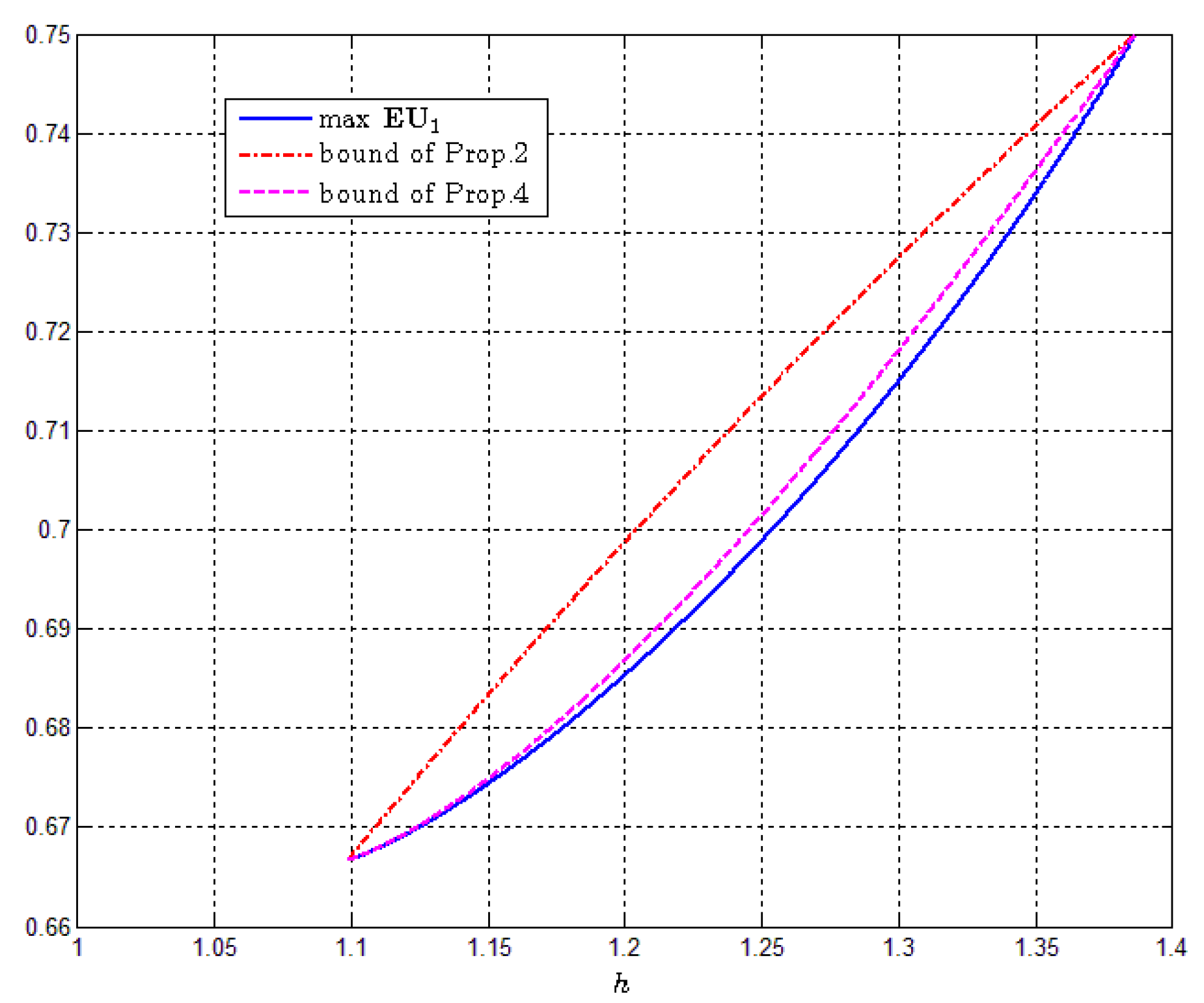
When $h=\ln n$ (or $k=\ln (n-1)$), there is an equality without the last term (see the proof of Proposition 3). At these points, the last term indeed vanishes. Inside the interval $\left(\ln \right(n-1),\ln n)$, Proposition 4 provides an improvement over Proposition 2. In Figure 1, we plot the exact value of max $\mathbb{E}{U}_1$ (calculated numerically using MATLAB) against the bounds of Propositions 2 and 4 for $h\in [\ln 3,\ln 4]$. It appears that the additional term in Proposition 4 captures most of the error in Proposition 2.

3. Proofs

Proof of Proposition 1.

Change the measure $\mathbf{p}$ by splitting some atom i into two atoms of sizes $p_i^{\prime }$ and $p_i^{\prime \prime }$ where $0<p_i^{\prime }<p_i$ and $p_i^{\prime \prime }=p_i-p_i^{\prime }$. Let $\tilde{\mathbf{p}}=(p_1,...,p_{i-1},p_i^{\prime },p_i^{\prime \prime },p_{i+1},...)$ be the new measure. The entropy of $\mathbf{p}$ is smaller than that of $\tilde{\mathbf{p}}$ since

$$\begin{array}{ccc}\hfill p_i\ln {\displaystyle \frac{1}{p_i}}& =& [p_i^{\prime }+p_i^{\prime \prime }]\ln {\displaystyle \frac{1}{p_i}}\hfill \\ & <& p_i^{\prime }\ln {\displaystyle \frac{1}{p_i^{\prime }}}+p_i^{\prime \prime }\ln {\displaystyle \frac{1}{p_i^{\prime \prime }}}.\hfill \end{array}$$

Now

$$\begin{array}{ccc}\hfill p_i{(1-p_i)}^t& =& [p_i^{\prime }+p_i^{\prime \prime }]{(1-p_i)}^t\hfill \\ & <& p_i^{\prime }{(1-p_i^{\prime })}^t+p_i^{\prime \prime }{(1-p_i^{\prime \prime })}^t,\hfill \end{array}$$

which implies that ${\mathbb{E}}_{\mathbf{p}}{U}_t<{\mathbb{E}}_{\tilde{\mathbf{p}}}{U}_t$. Similarly, splitting any number of atoms, we increase both the entropy and $\mathbb{E}{U}_t$.

Now, take the first atom, for example, and split it into k sub-atoms, the first $k-1$ of which are of size p each and the k-th of size $p^{\prime }$, where $0\le p\le \frac{p_1}{k}$ and $p^{\prime }=p_1-(k-1)p$, and k is still to be determined. The entropy of the new measure is

$$(k-1)p\ln \frac{1}{p}+(p_1-(k-1)p)\ln \frac{1}{p_1-(k-1)p}+\sum _{i=2}^{\infty }{p}_i\ln \frac{1}{p_i}.$$

For sufficiently large k and $p=\frac{p_1}{k}$, this entropy becomes arbitrarily large, and in particular exceeds h. Take such a k, and consider the entropy of the obtained measure as p grows continuously from 0 to $\frac{p_1}{k}$. For $p=0$, we have basically the original measure (and thus an entropy less than h), while for $p=\frac{p_1}{k}$ the entropy is larger than h. Hence for an appropriate intermediate value of p, the entropy is exactly h. The measure obtained for this p proves our claim. ☐

Proof of Theorem 1.

Write down the Lagrangian:

$$L(\mathbf{p},{\lambda }_1,{\lambda }_2)=\sum _{i=1}^n{p}_i{(1-p_i)}^t+{\lambda }_1\left(\sum _{i=1}^n{p}_i-1\right)+{\lambda }_2\left(\sum _{i=1}^n{p}_i\ln \frac{1}{p_i}-h\right).$$

The first-order conditions yield:

$$\frac{\partial L}{\partial p_i}={(1-p_i)}^t-t{p}_i{(1-p_i)}^{t-1}+{\lambda }_1-{\lambda }_2(\ln p_i+1)=0.$$

Denote:

$$f\left(x\right)={(1-x)}^t-tx{(1-x)}^{t-1}+{\lambda }_1-{\lambda }_2(\ln x+1),0<x<1.$$

We have:

$$f^{\prime }\left(x\right)=t{(1-x)}^{t-2}[x(t+1)-2]-\frac{{\lambda }_2}{x}.$$

We claim that $f^{\prime }$ vanishes at most three times in $(0,1)$. Indeed, $f^{\prime }\left(x\right)=0$ when

$$xt{(1-x)}^{t-2}[x(t+1)-2]={\lambda }_2.$$

(8)

Denote the left-hand side of (8) by $g\left(x\right)$. Then:

$$g^{\prime }\left(x\right)=-t{(1-x)}^{t-3}[t^2{x}^2+t(x-4)x+2].$$

For every two points $x_1,$$x_2$ for which (8) holds, there is an intermediate point $x_1<\xi <x_2$ such that $g^{\prime }\left(\xi \right)=0$. Now, $g^{\prime }$ clearly vanishes at no more than two points, so that (8) holds for at most three values of x. It follows that each $p_i$ assumes one of up to (the same) four values. ☐

Before we prove Theorem 2 we need two auxiliary lemmas. For $h\ge 0$, let $X_h$ be the subset of ${\ell }_1$ consisting of all non-increasing sequences $(p_1,p_2,\dots )$ satisfying the following properties:

• $p_i\ge 0$ for each i and ${\displaystyle \sum _{i=1}^{\infty }{p}_i=1.}$
• $H\left(\mathbf{p}\right)\le h.$

Lemma 1.

$X_h$ is compact under the ${\ell }_1$ metric.

Proof of Lemma 1.

Let ${\left({\mathbf{p}}_n\right)}_{n=1}^{\infty }$ be a sequence in $X_h$, say ${\mathbf{p}}_n=(p_{n1},p_{n2},\dots )$ for $n\ge 1$. We want to show that it has a convergent subsequence in $X_h$. Employing the diagonal method, we may assume that ${\mathbf{p}}_n$ converges component-wise. Let $\mathbf{p}=(p_1,p_2,\dots )$ be the limit. It is clear that $\mathbf{p}$ has non-negative and non-increasing entries, so we only need to show that ${\displaystyle \sum _{i=1}^{\infty }{p}_i=1}$, that $H\left(\mathbf{p}\right)\le h$, and that ${\mathbf{p}}_n\underset{n\to \infty }{⟶}\mathbf{p}$ in ${\ell }_1$.

Assume first that ${\displaystyle \sum _{i=1}^{\infty }{p}_i>1}$. Then, there exists an index $i_0$ such that ${\displaystyle \sum _{i=1}^{i_0}{p}_i>1}$. Hence for sufficiently large n, we have ${\displaystyle \sum _{i=1}^{i_0}{p}_{ni}>1}$, which is a contradiction. Hence ${\displaystyle \sum _{i=1}^{\infty }{p}_i\le 1}$. Now assume that ${\displaystyle \sum _{i=1}^{\infty }{p}_i<1}$. Put ${\displaystyle \epsilon =1-\sum _{i=1}^{\infty }{p}_i}$. Let $i_0$ be an integer, to be determined later. We have ${\displaystyle {\displaystyle \sum _{i=1}^{i_0}{p}_{ni}}<1-\frac{\epsilon }{2}}$ for all sufficiently large n. Note that for every $\mathbf{q}=(q_1,q_2,\dots )\in X_h$ we have $q_i\le {\displaystyle \frac{1}{i}}(q_1+q_2+\dots +q_i)\le {\displaystyle \frac{1}{i}}$. Now we can bound from below the tail entropy of ${\mathbf{p}}_n$:

$${\displaystyle {\displaystyle \sum _{i=i_0+1}^{\infty }{p}_{ni}\ln \frac{1}{p_{ni}}>\sum _{i=i_0+1}^{\infty }{p}_{ni}\ln i_0>\frac{\epsilon }{2}\ln i_0}}.$$

Taking $i_0$ large enough, we can make the right-hand side larger than h, which is impossible. Hence ${\displaystyle \sum _{i=1}^{\infty }{p}_i=1}$.

We now show similarly that $H\left(\mathbf{p}\right)\le h$. Assume that ${\displaystyle \sum _{i=1}^{\infty }{p}_i\ln \frac{1}{p_i}>h}$. Then there exists an $i_0$ such that ${\displaystyle \sum _{i=1}^{i_0}{p}_i\ln \frac{1}{p_i}>h}$. Then, however, ${\displaystyle \sum _{i=1}^{i_0}{p}_{ni}\ln \frac{1}{p_{ni}}>h}$ for sufficiently large n, which yields a contradiction.

To prove convergence in ${\ell }_1$, we estimate ${\displaystyle {∥{\mathbf{p}}_n-\mathbf{p}∥}_1=\sum _{i=1}^{\infty }|p_{ni}-p_i|}$. Let $\epsilon >0$. Since ${\displaystyle \sum _{i=1}^{\infty }{p}_i=1}$, we can find an $i_0$ such that ${\displaystyle \sum _{i=i_0+1}^{\infty }{p}_i<\frac{\epsilon }{6}}$. Due to the component-wise convergence, for sufficiently large n we have ${\displaystyle \sum _{i=1}^{i_0}|p_{ni}-p_i|<\frac{\epsilon }{6}}$. For such n we also have ${\displaystyle \sum _{i=i_0+1}^{\infty }{p}_{ni}<\frac{\epsilon }{3}}$ since

$$\begin{array}{lll}{\displaystyle \sum _{i=1}^{i_0}|p_{ni}-p_i|<\frac{\epsilon }{6}}& \Rightarrow & \left|\sum _{i=1}^{i_0}\left(p_{ni}-p_i\right)\right|<\frac{\epsilon }{6}\hfill \\ & \Rightarrow & \sum _{i=1}^{i_0}{p}_{ni}>\sum _{i=1}^{i_0}{p}_i-\frac{\epsilon }{6}>1-\frac{\epsilon }{3}\hfill \\ & \Rightarrow & {\displaystyle \sum _{i=i_0+1}^{\infty }{p}_{ni}<\frac{\epsilon }{3}}.\hfill \end{array}$$

Thus we have

$$\begin{array}{lll}{\displaystyle \sum _{i=1}^{\infty }|p_{ni}-p_i|}& =& {\displaystyle \sum _{i=1}^{i_0}|p_{ni}-p_i|}+\sum _{i=i_0+1}^{\infty }|p_{ni}-p_i|\hfill \\ & <& \frac{\epsilon }{6}+\sum _{i=i_0+1}^{\infty }|p_{ni}|+\sum _{i=i_0+1}^{\infty }\left|p_i\right|\hfill \\ & <& \frac{\epsilon }{6}+\frac{\epsilon }{3}+\frac{\epsilon }{6}<\epsilon .\hfill \end{array}$$

Hence we have convergence in ${\ell }_1$. This proves the lemma. ☐

Example 1.

Note that the subset of $X_h$ consisting of all those vectors whose entropy is exactly h is not compact. Let us demonstrate this fact, say, for $h=\ln 2$. We choose ${\displaystyle {\mathbf{p}}_n=(x_n,\underset{n\mathrm{times}}{\underbrace{\frac{1-x_n}{n},\frac{1-x_n}{n},\frac{1-x_n}{n},\dots ,\frac{1-x_n}{n}}})}$, $n\ge 3,$ where $x_n$ will be defined momentarily. For arbitrary fixed $n\ge 3$, put:

$$f_n\left(x\right)=-x\ln x-(1-x)\ln \frac{1-x}{n},0\le x\le 1.$$

We claim that there exists a unique solution $x_n$ to the equation $f_n\left(x\right)=\ln 2$. Indeed, this follows readily from the fact that $f_n\left(x\right)$ is concave and $f_n\left(1\right)=0<\ln 2<\ln n=f_n\left(0\right)$. Denoting $t_n=1-x_n$, we have

$$-(1-t_n)\ln \left(1-t_n\right)-t_n\ln t_n+t_n\ln n=\ln 2.$$

Hence

$$\begin{array}{ccc}\hfill t_n& =& \frac{1}{\ln n}\left(\ln 2+t_n\ln t_n+(1-t_n)\ln \left(1-t_n\right)\right)\le \frac{\ln 2}{\ln n},\hfill \end{array}$$

so that

$$x_n\ge 1-\frac{\ln 2}{\ln n},n\ge 3,$$

and in particular $x_n\underset{n\to \infty }{⟶}1$. Thus, ${\mathbf{p}}_n\underset{n\to \infty }{⟶}(1,0,0,0,\dots )$ while $H\left({\mathbf{p}}_n\right)=\ln 2$ and $H\left(\right(1,0,0,0,\dots \left)\right)=0$, which completes the example.

For arbitrary fixed t, the quantity $\mathbb{E}{U}_t$ assigns to each point in $X_h$ a real number. We will denote this function by $\mathbb{E}{U}_t$.

Lemma 2.

The mapping $\mathbb{E}{U}_t$: $X_h⟶\mathbb{R}$ is Lipschitz with constant 1 with respect to the ${\ell }_1$ metric.

Proof of Lemma 2.

Consider the function $f:[0,1]⟶\mathbb{R}$ given by $f\left(x\right)=x{(1-x)}^t,0\le x\le 1$. Let M be the Lipschitz constant for $f\left(x\right)$. According to Lemma 7 from [4], the candidates for assuming the maximum of $|f^{\prime }\left(x\right)|$ are the points $x_1=0$ and $x_2=\frac{2}{1+t}$. Now $|f^{\prime }\left(x_1\right)|=1$ and $|f^{\prime }\left(x_2\right)|={(1-\frac{2}{1+t})}^{t-1}\le 1$. Hence the Lipschitz constant for $f\left(x\right)$ is 1. It follows that if $\mathbf{p},{\mathbf{p}}^{\prime }\in X_h$, then:

$$\begin{array}{lll}\left|{\displaystyle \sum _{i=1}^{\infty }{p}_i{(1-p_i)}^t-\sum _{i=1}^{\infty }{p}_i^{\prime }{(1-p_i^{\prime })}^t}\right|& =& \left|{\displaystyle \sum _{i=1}^{\infty }\left(p_i{(1-p_i)}^t-p_i^{\prime }{(1-p_i^{\prime })}^t\right)}\right|\hfill \\ & \le & \sum _{i=1}^{\infty }\left|p_i-p_i^{\prime }\right|.\hfill \end{array}$$

 ☐

Proof of Theorem 2.

(i) 

Follows from Lemma 1 and Lemma 2.

(ii) 

Suppose that $\mathbf{p}=(p_1,p_2,\dots )$ does not have a finite support. Then, we can find an $n_0$ such that the first $n_0$ entries $p_1,p_2,\dots ,p_{n_0}$ of $\mathbf{p}$ assume more than four different values. Put $\tilde{\mathbf{p}}=(p_1,p_2,\dots ,p_{n_0})$ and let $c=p_1+p_2+\dots +p_{n_0}$ and $\tilde{h}=H\left(\tilde{\mathbf{p}}\right)$. Consider the optimization problem

$$\begin{array}{cc}\hfill \underset{\mathbf{p}}{\max }& \sum _{i=1}^{n_0}{p}_i{(1-p_i)}^t\hfill \end{array}$$

(9)

subject to

$$\begin{array}{}\mathrm{(10)}& \sum _{i=1}^{n_0}{p}_i\ln \frac{1}{p_i}\le \tilde{h},\hfill \mathrm{(11)}& \sum _{i=1}^{n_0}{p}_i=c.\hfill \end{array}$$

Theorem 1 is still applicable to (9)–(11) with a minor variation. In the beginning of the proof, replace the Lagrangian by

$$L(\mathbf{p},{\lambda }_1,{\lambda }_2)=\sum _{i=1}^n{p}_i{(1-p_i)}^t+{\lambda }_1\left(\sum _{i=1}^n{p}_i-c\right)+{\lambda }_2\left(\sum _{i=1}^n{p}_i\ln \frac{1}{p_i}-\tilde{h}\right)$$

and proceed as previously. Since $\mathbf{p}\in X_h$ maximizes $\mathbb{E}{U}_t$, the vector $\tilde{\mathbf{p}}$ is a global optimum of this finite-dimensional problem. By Theorem 1, $\tilde{\mathbf{p}}$ cannot assume more than four distinct values.

 ☐

Proof of Theorem 3.

For $0<x<1:$

$$\begin{array}{lll}\ln (1-x)& =& -x-\frac{x^2}{2}-\dots -\frac{x^{2t-1}}{2t-1}-\dots \hfill \\ & <& -x-\frac{x^2}{2}-\dots -\frac{x^{2t-1}}{2t-1}\hfill \\ & =& \left(-x-\frac{x^{2t-1}}{2t-1}\right)+\dots +\left(-\frac{x^{t-k}}{t-k}-\frac{x^{t+k}}{t+k}\right)\hfill \\ & & +\dots +\left(-\frac{x^{t-1}}{t-1}-\frac{x^{t+1}}{t+1}\right)-\frac{x^t}{t}.\hfill \end{array}$$

(12)

For each term on the right-hand side of (12) and for $1\le k\le t-1$, we have

$$-\frac{x^{t-k}}{t-k}-\frac{x^{t+k}}{t+k}<-\frac{x^t}{t-k}-\frac{x^t}{t+k}.$$

Indeed,

$$-\frac{x^{t-k}}{t-k}-\frac{x^{t+k}}{t+k}+\frac{x^t}{t-k}+\frac{x^t}{t+k}=-x^{t-k}(1-x^k)(\frac{1}{t-k}-\frac{x^k}{t+k})<0.$$

This gives us

$$-x-\frac{x^2}{2}-\dots -\frac{x^{2t-1}}{2t-1}-\dots <-x^t-\frac{x^t}{2}-\dots -\frac{x^t}{t}-\dots -\frac{x^t}{2t-1}<-x^t{H}_{2t-1}.$$

Hence

$$\ln p<-{(1-p)}^t{H}_{2t-1},$$

and therefore

$${(1-p)}^t<-\frac{\ln p}{H_{2t-1}}.$$

Finally,

$$\mathbb{E}{U}_t=\sum _{i=1}^{\infty }{p}_i{(1-p_i)}^t\le {\displaystyle \frac{h}{H_{2t-1}}}.$$

 ☐

Proof of Theorem 4.

Let $t>1$ be an integer and $\alpha >1$. Define $\mathbf{p}$ by:

$$p_1=p_2=\dots =p_t=\frac{h}{\sqrt{\alpha }t\ln t},p_{t+1}=1-\frac{h}{\sqrt{\alpha }\ln t}.$$

For such t:

$$\begin{array}{lll}{\mathbb{E}}_{\mathbf{p}}{U}_t& =& \left(1-\frac{h}{\sqrt{\alpha }\ln t}\right){\left(\frac{h}{\sqrt{\alpha }\ln t}\right)}^t+\frac{h}{\sqrt{\alpha }\ln t}{\left(1-\frac{h}{\sqrt{\alpha }t\ln t}\right)}^t\hfill \\ & \ge & \frac{h}{\sqrt{\alpha }\ln t}{\left(1-\frac{h}{\sqrt{\alpha }t\ln t}\right)}^t.\hfill \end{array}$$

Now:

$${\left(1-\frac{h}{\sqrt{\alpha }t\ln t}\right)}^t={\left({\left(1-\frac{h}{\sqrt{\alpha }t\ln t}\right)}^{t\ln t}\right)}^{1/\ln t}\underset{t\to \infty }{⟶}{\left(e^{-h/\sqrt{\alpha }}\right)}^0=1.$$

 ☐

Proof of Proposition 2.

Let P be the random variable assigning to each atom $i\in S$ its probability:

$$P\left(i\right)=p_i,i\in S.$$

Denote $I=-\ln P$. Then:

$$\mathbb{E}{U}_1=\sum _{i\in S}{p}_i(1-p_i)=\mathbb{E}[1-P]=\mathbb{E}[1-e^{-I}].$$

The function $f\left(x\right)=1-e^{-x}$ is concave, so by Jensen’s inequality:

$$\begin{array}{lll}\mathbb{E}{U}_1& =& \mathbb{E}[1-e^{-I}]\hfill \\ & \le & 1-e^{-\mathbb{E}\left[I\right]}\hfill \\ & =& 1-e^{-\mathbb{E}[-\ln P]}\hfill \\ & =& 1-e^{{\sum }_{i\in S}{p}_i\ln p_i}\hfill \\ & =& 1-e^{-h}.\hfill \end{array}$$

 ☐

Remark 2.

If $h=\ln k$ for some positive integer k, then the bound is attained for the uniform distribution on a space of k points.

Proof of Proposition 3.

First, in the case where $h=\ln k$ we have a unique optimal solution, which is $p_1^{*}=p_2^{*}=\dots =p_{n-k}^{*}=0<p_{n-k+1}^{*}=p_{n-k+2}^{*}=\dots =p_n^{*}={\displaystyle \frac{1}{k}}$. It is straightforward to check that ${\mathbf{p}}^{*}$ is feasible and attains the upper bound in Proposition 2, and is optimal. Moreover, ${\mathbf{p}}^{*}$ is unique because any feasible non-uniform choice of ${\mathbf{p}}^{*}$ leads to a strict inequality in Jensen’s inequality that was used in Proposition 2.

Thus, we deal with the case of strict inequalities, $\ln (k-1)<h<\ln k$. We start by showing that any optimal solution $(p_1^{*},p_2^{*},\dots ,p_n^{*})$ assumes at most two non-zero distinct values. Write down the Lagrangian:

$$L(p_1,p_2,\dots ,p_n,{\lambda }_1,{\lambda }_2)=\sum _{i=1}^n{p}_i(1-p_i)+{\lambda }_1\left(\sum _{i=1}^n{p}_i-1\right)+{\lambda }_2\left(\sum _{i=1}^n{p}_i\ln \frac{1}{p_i}-h\right).$$

The first-order conditions yield, at any optimal point,

$$\frac{\partial L}{\partial p_i}=1-2p_i+{\lambda }_1-{\lambda }_2\left(\ln p_i+1\right)=0,$$

for every i with $p_i^{*}>0$. Define the function f by $f\left(x\right)=1-2x+{\lambda }_1-{\lambda }_2-{\lambda }_2\ln x$. The function vanishes at most twice in $(0,1)$ because its derivative $f^{\prime }\left(x\right)=-2-{\displaystyle \frac{{\lambda }_2}{x}}$ vanishes at most once. Thus, the non-zero $p_i^{*}$s assume at most two distinct values. In fact, if all were equal, we would have $k=\ln k$, where k is the number of non-zero $p_i^{*}$s, so that we would have exactly two distinct values for the $p_i^{*}$s. Disposing of the points of mass 0, we may assume that all n points of S have positive mass. Denote the number of “light” atoms by ℓ. We will show that $\mathbb{E}{U}_1$ decreases as we increase ℓ. Denote the mass of a “light” atom by p and write down the entropy constraint with ℓ “light” atoms and $n-\ell$ “heavy” ones:

$$-\ell p\ln p-(1-\ell p)\ln \left(\frac{1-\ell p}{n-\ell }\right)=h.$$

Now, define the function $F(\ell ,p)$ by:

$$F(\ell ,p)=-\ell p\ln p-(1-\ell p)\ln \left(\frac{1-\ell p}{n-\ell }\right)-h.$$

Note that we treat ℓ as a continuous variable. The equation $F(\ell ,p)=0$ implicitly defines the function $p\left(\ell \right)$. Using the implicit function theorem, we can write an analytic expression for ${\displaystyle \frac{dp}{d\ell }}$:

$${\displaystyle \frac{dp}{d\ell }}=-\frac{p\left(\ell \right)}{\ell }+\frac{{\displaystyle \frac{1-\ell p\left(\ell \right)}{n-\ell }}-p\left(\ell \right)}{\ell \left[\ln \left({\displaystyle \frac{1-\ell p\left(\ell \right)}{n-\ell }}\right)-\ln p\left(\ell \right)\right]}.$$

Now write down $\mathbb{E}{U}_1$ as a function of ℓ and take the derivative with respect to ℓ:

$$\mathbb{E}{U}_1=\ell p\left(\ell \right)(1-p\left(\ell \right))+(1-\ell p\left(\ell \right))\left(1-\frac{1-\ell p\left(\ell \right)}{n-\ell }\right).$$

$$\begin{array}{lll}\frac{d\mathbb{E}{U}_1}{d\ell }& =& \left(p\left(\ell \right)+\ell p^{\prime }\left)\right(\ell \right)\left(1-p\left(\ell \right)\right)-\ell p\left(\ell \right)p^{\prime }\left(\ell \right)\hfill \\ & & -\left(p\left(\ell \right)+\ell p^{\prime }\left(\ell \right)\right)\left(1-\frac{1-\ell p\left(\ell \right)}{n-\ell }\right)\hfill \\ & & -\frac{\left(1-\ell p\left(\ell \right)\right)}{{\left(n-\ell \right)}^2}\left(-np\left(\ell \right)-n\ell p^{\prime }\left(\ell \right)+{\ell }^2{p}^{\prime }\left(\ell \right)+1\right).\hfill \end{array}$$

(13)

Notice that the term ${\displaystyle \frac{1-\ell p\left(\ell \right)}{n-\ell }}$ is actually the mass of the “heavy” atom, so to simplify notation we put $q\left(\ell \right)={\displaystyle \frac{1-\ell p\left(\ell \right)}{n-\ell }}$. Substituting the expression for ${\displaystyle \frac{dp}{d\ell }}$, we obtain:

$$\begin{array}{lll}\frac{\partial \mathbb{E}{U}_1}{\partial \ell }& =& {\left(q\left(\ell \right)-p\left(\ell \right)\right)}^2\left[\frac{2}{\ln \frac{q\left(\ell \right)}{p\left(\ell \right)}}-\frac{2p\left(\ell \right)}{q\left(\ell \right)-p\left(\ell \right)}-1\right]\hfill \\ & =& {\left(q\left(\ell \right)-p\left(\ell \right)\right)}^2\left[\frac{2}{\ln \frac{q\left(\ell \right)}{p\left(\ell \right)}}-\frac{2}{\frac{q\left(\ell \right)}{p\left(\ell \right)}-1}-1\right].\hfill \end{array}$$

(14)

To show that $\mathbb{E}{U}_1$ decreases as we increase ℓ, it is enough to check that $\frac{\partial \mathbb{E}{U}_1}{\partial \ell }<0$. It suffices to work out the second term in the product of (14). Using the change of variables $y=\frac{q\left(\ell \right)}{p\left(\ell \right)}-1$, we may write:

$$\frac{2}{\ln \frac{q\left(\ell \right)}{p\left(\ell \right)}}-\frac{2}{\frac{q\left(\ell \right)}{p\left(\ell \right)}-1}-1=\frac{2}{\ln \left(1+y\right)}-\frac{2}{y}-1.$$

It is straightforward to check that $\frac{2}{\ln \left(1+y\right)}-\frac{2}{y}-1\le 0$:

$$\begin{array}{ccc}\hfill \frac{2}{\ln \left(1+y\right)}-\frac{2}{y}-1& =& \frac{2y-2\ln \left(1+y\right)-y\ln \left(1+y\right)}{y\ln \left(1+y\right)}.\hfill \end{array}$$

Notice that $y\ln \left(1+y\right)>0$, and hence it is enough to check that the numerator is negative. Indeed,

$${\left[2y-2\ln \left(1+y\right)-y\ln \left(1+y\right)\right]}_{y=0}=0$$

and

$$\frac{d}{dy}\left[2y-2\ln \left(1+y\right)-y\ln \left(1+y\right)\right]=\frac{y}{1+y}-\ln \left(1+y\right).$$

Now ${[\frac{y}{1+y}-\ln \left(1+y\right)]}_{y=0}=0$ and $\frac{d}{dy}\left[\frac{y}{1+y}-\ln \left(1+y\right)\right]=\frac{1}{{\left(1+y\right)}^2}-\frac{1}{1+y}<0$. Thus, $\frac{\partial \mathbb{E}{U}_1}{\partial \ell }<0$.

It follows that ℓ should be as small as possible, which means (since there is at least one light atom) that $\ell =1$. Finally, as there is one light atom and $n-1$ heavy ones, the entropy h lies in the interval $\left(\ln \right(n-1),\ln n)$. Reverting to the original notations, we have $\ln (k-1)<h<\ln k$. ☐

Proof of Proposition 4.

We use the following refinement of Jensen’s inequality [11]: For any random variable X and concave function $\varphi$,

$$\begin{array}{cc}\hfill \varphi \left(\mathbb{E}\left(X\right)\right)-\mathbb{E}\left(\varphi \left(X\right)\right)\ge & \left|\mathbb{E}\left(\left|\varphi \left(X\right)-\varphi \left(\mathbb{E}\left(X\right)\right)\right|\right)-\left|{\varphi }_{+}^{{}^{\prime }}\left(\mathbb{E}\left(X\right)\right)\right|·\mathbb{E}\left(\left|X-\mathbb{E}\left(X\right)\right|\right)\right|,\hfill \end{array}$$

(15)

where ${\varphi }_{+}^{\prime }$ denotes the right-hand derivative of $\varphi$. For $I=-\ln P$ and $\varphi \left(x\right)=1-e^{-x}$, the left-hand side of (15) is

$$\varphi \left(\mathbb{E}\left[I\right]\right)-\mathbb{E}\left[\varphi \left(I\right)\right]=1-e^{-h}-\mathbb{E}{U}_1.$$

The right-hand side of (15) gives:

$$\begin{array}{c}\left|\mathbb{E}\left(\left|\varphi \left(I\right)-\varphi \left(\mathbb{E}\right[I\left]\right)\right|\right)-\left|{\varphi }_{+}^{{}^{\prime }}\left(\mathbb{E}\left[I\right]\right)\right|·\mathbb{E}\left(\left|I-E\left[I\right]\right|\right)\right|\hfill \\ =\left|\mathbb{E}\left(\left|1-e^{-I}-\left(1-e^{-h}\right)\right|\right)-e^{-h}\mathbb{E}\left(\left|-\ln P-h\right|\right)\right|\hfill \\ =|p·\left|e^{-h}-p\right|+\left(n-1\right)q·\left|e^{-h}-q\right|\hfill \\ -e^{-h}\left(p·\left|-\ln p-h\right|+\left(n-1\right)q·\left|-\ln q-h\right|\right)|\hfill \\ =|p\left(e^{-h}-p\right)-\left(n-1\right)q\left(e^{-h}-q\right)\hfill \\ -e^{-h}\left(p\left(-\ln p-h\right)-\left(n-1\right)q\left(-\ln q-h\right)\right)|\hfill \\ =\left|p{e}^{-h}-p^2-\left(n-1\right)q{e}^{-h}+\left(n-1\right)q^2-e^{-h}\left(-2p\ln p-h-2ph+h\right)\right|\hfill \\ =\left|e^{-h}\left(2p-1+2p\ln p+2ph\right)+\left(n-1\right)q^2-p^2\right|.\hfill \end{array}$$

 ☐

References

- Good, I.J. The Population Frequencies of Species and the Estimation of Population Parameters. Biometrika 1953, 40, 237–264. [Google Scholar] [CrossRef]
- McAllester, D.; McAllester, R.E. On The Convergence Rate of Good-Turing Estimators. In Proceedings of the Thirteenth Annual Conference on Computational Learning Theory, Stanford, CA, USA, 28 June–1 July 2000; pp. 1–6. [Google Scholar]
- Haslinger, R.; Pipa, G.; Lewis, L.D.; Nikolić, D.; Williams, Z.; Brown, E. Encoding through Patterns: Regression Tree-Based Neuronal Population Models. Neural Comput. 2013, 25, 1953–1993. [Google Scholar] [CrossRef] [PubMed]
- Berend, D.; Kontorovich, A. The Missing Mass Problem. Stat. Probab. Lett. 2012, 82, 1102–1110. [Google Scholar] [CrossRef]
- Berend, D.; Kontorovich, A. On The Concentration of the Missing Mass. Electron. Commun. Probab. 2013, 18, 1–7. [Google Scholar] [CrossRef]
- Kontorovich, A.; Hendler, D.; Menahem, E. Metric Anomaly Detection via Asymmetric Risk Minimization. In SIMBAD 2011. Lecture Notes in Computer Science; Springer: Berlin/Heidelberg, Germany, 2011; Volume 7005, pp. 17–30. [Google Scholar]
- Luo, H.P.; Schapire, R. Towards Minimax Online Learning with Unknown Time Horizon. In Proceedings of the 31st International Conference on International Conference on Machine Learning, Beijing, China, 21–26 June 2014. [Google Scholar]
- Sadeqi, M.; Holte, R.C.; Zilles, S. Detecting Mutex Pairs in State Spaces by Sampling. In Australasian Conference on Artificial Intelligence (2013); Lecture Notes in Computer Science; Springer: Cham, Switzerland; Volume 8272, pp. 490–501.
- Ben-Hamou, A.; Boucheron, S.; Ohannessian, M.I. Concentration Inequalities in the Infinite Urn Scheme for Occupancy Counts and the Missing Mass, with Applications. Bernoulli 2017, 23, 249–287. [Google Scholar] [CrossRef]
- Han, Y.J.; Jiao, J.T.; Weissman, T. Minimax Estimation of Discrete Distributions under ℓ1 Loss. IEEE Trans. Inf. Theory 2015, 61, 6343–6354. [Google Scholar] [CrossRef]
- Hussain, S.; Pečarić, J. An Improvement of Jensen’s Inequality with Some Applications. Asian Eur. J. Math. 2009, 2, 85–94. [Google Scholar] [CrossRef]
Figure 1.
Max vs. the bounds provided by Propositions 2 and 4.
© 2017 by the authors. Licensee MDPI, Basel, Switzerland. This article is an open access article distributed under the terms and conditions of the Creative Commons Attribution (CC BY) license (http://creativecommons.org/licenses/by/4.0/).
Share and Cite
MDPI and ACS Style
Berend, D.; Kontorovich, A.; Zagdanski, G. The Expected Missing Mass under an Entropy Constraint. Entropy 2017, 19, 315. https://doi.org/10.3390/e19070315
AMA Style
Berend D, Kontorovich A, Zagdanski G. The Expected Missing Mass under an Entropy Constraint. Entropy. 2017; 19(7):315. https://doi.org/10.3390/e19070315
Chicago/Turabian StyleBerend, Daniel, Aryeh Kontorovich, and Gil Zagdanski. 2017. "The Expected Missing Mass under an Entropy Constraint" Entropy 19, no. 7: 315. https://doi.org/10.3390/e19070315
Note that from the first issue of 2016, this journal uses article numbers instead of page numbers. See further details here.