On Unsteady Three-Dimensional Axisymmetric MHD Nanofluid Flow with Entropy Generation and Thermo-Diffusion Effects on a Non-Linear Stretching Sheet

Abstract

The entropy generation in unsteady three-dimensional axisymmetric magnetohydrodynamics (MHD) nanofluid flow over a non-linearly stretching sheet is investigated. The flow is subject to thermal radiation and a chemical reaction. The conservation equations are solved using the spectral quasi-linearization method. The novelty of the work is in the study of entropy generation in three-dimensional axisymmetric MHD nanofluid and the choice of the spectral quasi-linearization method as the solution method. The effects of Brownian motion and thermophoresis are also taken into account. The nanofluid particle volume fraction on the boundary is passively controlled. The results show that as the Hartmann number increases, both the Nusselt number and the Sherwood number decrease, whereas the skin friction increases. It is further shown that an increase in the thermal radiation parameter corresponds to a decrease in the Nusselt number. Moreover, entropy generation increases with respect to some physical parameters.

1. Introduction

The study of unsteady nanofluid flow, heat and mass transfers along a nonlinear stretching surface has received considerable attention during the last few years because of several applications in engineering processes, such as in materials manufacturing through extrusion, glass-fiber and paper production. Similarly, unsteady mixed convection in boundary layer flows have received attention with a large number of studies focusing on heat and mass transfer characteristics in nanofluids (Dessie et al. [1]). Nanofluids have increased thermal conductivity and convective heat transfer performance as compared to base fluids such as water and oils. The notion of a nanofluid was introduced by Choi [2] when he proposed the suspension of nanoparticles in a base fluid like water, oil or an ethylene-glycol mixture. These common base fluids have lower thermal conductivity, which is increased when nanoparticles are added. The increase in the thermal conductivity was explained by Buongiorno [3] in terms of the effect of particle Brownian motion and thermophoresis. Nanofluids have several applications due to the unique chemical and physical properties of the constituent nanoparticles. For instance, nanofluids have been used in applications that require high-performance cooling systems such as hot rolling, glass fiber production, rubber and the manufacture of metallic sheets [4].

Heat transfers due to free and mixed convection have several applications, for instance in electronic cooling, heat exchangers, etc. The study of axisymmetric magnetohydrodynamics (MHD) flow and heat transfer of power law fluid along an unsteady radially-stretching sheet was carried out by Ahmed et al. [5]. The conservation equations are solved analytically and numerically. Mohammadiun et al. [6] derived an exact solution of axisymmetric stagnation-point flow and heat transfer along a stationary infinite circular cylinder of a steady viscous compressible fluid with constant heat flux. The general self-similar solution was obtained with constant wall heat flux. The solutions of the system were obtained for different Reynolds numbers, compressibility factors and Prandtl numbers. Xiao et al. [7] proposed a mathematical model for heat convection in the presence of Brownian motion of nanoparticles where the physical properties of the fluid are predicted by the mean of fractal geometry. Thermal conductivity was found to have a positive and negative relation with concentration and the size of nanoparticles, respectively. The model output was found to be in good agreement with experimental data. Cai et al. [8] presented a review of research conducted on thermal conductivity and convective heat transfer in nanofluids by using fractal models and fractal-based techniques. Cai et al. [8] presented a model that considered the fractal distribution of nanoparticle sizes and heat convection between the fluid and the nanoparticles. Additionally, the heat transfer in nanofluids was modeled using three fractal-based models. The models were used to derive formulas for predicting the heat flux for boiling heat transfer. The predictions were found to be in a good agreement with the experimental data.

Shankar et al. [9] studied MHD flow, heat and mass transfer in a nanofluid flow along a stretching boundary with a non-uniform heat source/sink. The system of equations was solved using the Keller-box method. MHD effects in heat transfer have applications in science and technology. In MHD flow, the induced currents in the fluid generate forces, which in turn modify the flow field. Shahzad et al. [10] presented the exact solution for the MHD flow and heat transfer for a viscous incompressible fluid and a nonlinear sheet stretching radially in a porous medium.

Thermal radiation is important in the flow of a fluid, and consequently, the effects of thermal radiation on heat and mass transfer have been extensively studied. Ahmad et al. [11] considered the effect of thermal radiation on the steady MHD axisymmetric stagnation point flow of a viscous incompressible micropolar fluid along a shrinking sheet. The system of equations was solved numerically using an algorithm based on finite difference approximations. They found that the thickness of the thermal boundary layer becomes thinner as the thermal radiation parameter increased. The effect of melting heat transfer and second order slip with thermal radiation for a stagnation point flow was examined by Mabood et al. [12]. Singh et al. [13] analyzed unsteady MHD flow of a viscous incompressible fluid over a permeable stretching sheet and took into account the effect of thermal radiation.

In practical applications, mass transfer occurs due to molecular diffusion of species in homogeneous and heterogeneous chemical reactions (Sarada et al. [14]). The properties of the fluid can be affected by the diffusion of the species, which can either be generated or absorbed by the fluid. For this reason, the study of a chemical reaction in a fluid flow has attracted many researchers. Sarada et al. [14] analyzed the influence of a chemical reaction on unsteady MHD flow of a viscous incompressible fluid passing through an infinite vertical porous plate with varying suction.

The study of the unsteady flow of a viscous incompressible fluid along a linear stretching with a chemical reaction was investigated by Hunegnaw et al. [15]. They used a shooting technique and a fourth-order Runge–Kutta integration scheme combined with the Newton–Raphson method to solve the conservation equations. Barik [16] presented a study of the effects of a chemical reaction on unsteady rotating MHD flow in a porous medium with a heat source.

Entropy generation plays a vital role in the study of heat transfer processes. Entropy is a measure of the randomness or molecular disorder of a system. In accordance with the second law of thermodynamics, the entropy of a system always increases during an irreversible process and remains constant during a reversible process, that is entropy generation $\left(E_{gen}\right)$ is always positive for an irreversible process and zero for reversible process. The performance of any engineering system is degraded by irreversibility, and entropy generation is a measure of the magnitude of the irreversibility of the process.

Entropy generation is disregarded in most of the studies reviewed earlier. In this work, the mechanisms for generating entropy are connected to heat transfer, fluid friction irreversibility, magnetic field and mass transfer. The pioneering work in the analysis of entropy generation was done by Bejan [17]. Subsequently, entropy generation in MHD Casson nanofluid flow in the proximity of a stagnation point was investigated by Qing et al. [18]. The findings suggested a positive correlation between entropy generation and an increase in the Brinkman number, Reynolds number, Hartmann number and porosity. The study of entropy generation with MHD flow peristaltic blood of nanofluid across a porous medium was considered by Rashidi et al. [19]. The system was solved numerically using the homotopy perturbation method (HPM). The entropy generation of MHD an Eyring–Powell nanofluid flow towards a permeable stretching surface in the presence of nonlinear thermal radiation was investigated by Bhatti et al. [20]. The successive linearization method (SLM) and Chebyshev spectral collocation method are used. Rashidi et al. [21] studied entropy generation in nanofluid flow along a permeable stretching surface near the stagnation point with heat generation/absorption and a convective boundary condition. Bhatti et al. [22] used the successive linearization method (SLM) to study the entropy generation on non-Newtonian Carreau nanofluid over a shrinking sheet. The thermal radiation and magnetohydrodynamics (MHD) are taken into account. The idea of entropy generation in nanofluids is a growing area of research, and recent studies have examined different source terms and flow geometries [23].

The spectral quasi-linearization method (SQLM) has not been previously used to solve equations for three-dimensional axisymmetric MHD nanofluid flow. Moreover, to the best of the authors’ knowledge, entropy generation in this type of fluid flow has not been previously studied. The aim of the study is to analyze thermo-diffusion effects in three-dimensional axisymmetric MHD nanofluid flow, heat and mass transfers over a nonlinearly circular stretching sheet with entropy generation. The flow is subjected to thermal radiation and a chemical reaction. The conservation equations are solved numerically using the spectral quasi-linearization method [24]. The SQLM combines fast convergence with accuracy. The method has been used in recent boundary layer flow and heat transfer studies, such as [24,25]. In addition, the nanofluid boundary condition suggested by Nield and Kuznetsov [26] is adopted where it is assumed that the nanoparticle mass flux at the wall vanishes. The results are found to be in good agreement with previously published work, such as Mustafa et al. [27].

2. Problem Formulation

Consider the unsteady three-dimensional MHD flow of an incompressible viscous flow of nanofluid. A cylindrical coordinate system $(r,\theta ,z)$ is used. The velocity of the stretching sheet is assumed to be nonlinear along the radial direction. It is assumed that there is no nanoparticle flux across the wall, and the surface is stretching along the z-direction. In the ambient fluid, the temperature, solute concentration and nanoparticle concentration are denoted by $T_{\infty },C_{\infty }$ and ${\psi }_{\infty }$, respectively (see Figure 1). Here, $C_w$, $T_w$ and ${\psi }_w$ represent the solute concentration, constant temperature and nanoparticle concentration respectively on the wall. The variable magnetic field intensity is denoted by $B(r,t)$ where t represents time. The magnetic field acts in the positive z-direction normal to the sheet. In this study, $B(r,t)$ generalizes the magnetic field term provided previously in [9,10] to:

$$\begin{array}{c}\hfill B(r,t)=\frac{B_0{r}^{(n-1)/2}}{\sqrt{1-\lambda t}},\end{array}$$

(1)

where $B_0$ is the uniform magnetic field strength, $n>0$ is the power-law index or stretching sheet parameter and $\lambda$ represents the unsteadiness parameter.

The equations for the conservation of momentum, energy, mass and nanoparticle volume fraction, considering the boundary layer assumptions presented above, can be obtained [27,28] as:

$$\begin{array}{cc}\hfill & \frac{\partial u}{\partial r}+\frac{u}{r}+\frac{\partial w}{\partial z}=0,\hfill \end{array}$$

(2)

$$\begin{array}{cc}\hfill & \frac{\partial u}{\partial t}+u\frac{\partial u}{\partial r}+w\frac{\partial u}{\partial z}={\nu }_f\frac{{\partial }^{2}u}{\partial z^2}-\frac{\sigma B^2(r,t)u}{{\rho }_f},\hfill \end{array}$$

(3)

$$\begin{array}{cc}\hfill & \frac{\partial T}{\partial t}+u\frac{\partial T}{\partial r}+w\frac{\partial T}{\partial z}={\alpha }_f\frac{{\partial }^{2}T}{\partial z^2}+\tau \left[D_B\frac{\partial \psi }{\partial z}\frac{\partial T}{\partial z}+\frac{D_T}{T_{\infty }}{\left(\frac{\partial T}{\partial z}\right)}^2\right]+D_{TC}\frac{{\partial }^{2}C}{\partial z}-\frac{1}{{\rho }_f{c}_p}\frac{\partial q_r}{\partial z},\hfill \end{array}$$

(4)

$$\begin{array}{c}\frac{\partial C}{\partial t}+u\frac{\partial C}{\partial r}+w\frac{\partial C}{\partial z}=D_s\frac{{\partial }^{2}C}{\partial z^2}+D_{CT}\frac{{\partial }^{2}T}{\partial z}-R(r,t)(C-C_{\infty }),\hfill \end{array}$$

(5)

$$\begin{array}{c}\frac{\partial \psi }{\partial t}+u\frac{\partial \psi }{\partial r}+w\frac{\partial \psi }{\partial z}=D_B\frac{{\partial }^2\psi }{\partial z^2}+\frac{D_T}{T_{\infty }}\frac{{\partial }^{2}T}{\partial z^2},\hfill \end{array}$$

(6)

where u and w represent the fluid velocity components in r and z directions, respectively; ${\nu }_f$, $\sigma$ and ${\rho }_f$ are the kinematic viscosity, electrical conductivity and the density of the fluid, respectively; ${\alpha }_f=k_f/{\left(\rho c_p\right)}_f$ is the thermal diffusivity, $c_p$ is the heat capacity, $D_B$ is the Brownian diffusion coefficient, $D_T$ is the thermophoretic diffusion coefficient; $\tau ={\left(\rho c_p\right)}_s/{\left(\rho c_p\right)}_f$ the ratio of effective heat capacity of the nanoparticle material to heat capacity of the fluid; $D_{CT}$ and $D_{TC}$ are the Soret and Dufour diffusivities, $D_s$ is the solute diffusivity and $R(r,t)$ is the chemical reaction.

The quantity $q_r$ is the relative heat flux. Applying the Rosseland approximation, [29], $q_r$ can be expressed as:

$$\begin{array}{c}\hfill q_r=-\frac{4{\sigma }^{\ast }}{3K^{\ast }}\frac{\partial T^4}{\partial z},\end{array}$$

(7)

In Equation (7), ${\sigma }^{\ast }$ is the Stefan–Boltzmann constant while $K^{\ast }$ is the Rosseland mean spectral absorption coefficient. If the variation in temperature across the flow is small, $T^4$ may be expanded using the Taylor series about $T_{\infty }$, which yields:

$$\begin{array}{c}\hfill T^4\approxeq 4T_{\infty }^{3}T-3T_{\infty }^4.\end{array}$$

(8)

Substituting Equation (8) in Equation (7), the relative heat flux becomes:

$$\begin{array}{c}\hfill q_r=-\frac{16{\sigma }^{\ast }{T}_{\infty }^3}{3K^{\ast }}\frac{\partial T}{\partial z}.\end{array}$$

(9)

To simplify the mass equation, the chemical reaction $R(r,t)$ must be a constant. This condition holds if $R(r,t)$ has the following form:

$$\begin{array}{c}\hfill R(r,t)=R_0\frac{a{r}^{n-1}}{1-\lambda t},\end{array}$$

(10)

where $R_0$ is constant and $a>0$ is the stretching constant.

The boundary conditions considered (see [27]) are:

$$\begin{array}{c}\hfill u=u_w\left(r\right)=\frac{a{r}^n}{1-\lambda t},-k_f\frac{\partial T}{\partial z}=h_f(T_w-T),\\ \hfill D_B\frac{\partial \psi }{\partial z}+\frac{D_T}{T_{\infty }}\frac{\partial T}{\partial z}=0,C=C_{w}atz=0,\\ \hfill u\to 0,T\to T_{\infty },C\to C_{\infty }\mathrm{and}\\ \hfill \psi \to {\psi }_{\infty }\mathrm{as}z\to \infty ,\end{array}$$

(11)

where $k_f=k_0\sqrt{1-\lambda t}$ is the thermal conductivity of the base fluid where $k_0$ is a constant. A similarity solution of the energy equation can be obtained if the Biot number,

$$\begin{array}{c}Bi=\frac{h_f}{k_0}\sqrt{\frac{{\nu }_f}{a{r}^{(n-1)}}},\hfill \end{array}$$

(12)

is a constant. This condition is satisfied if the heat transfer coefficient, $h_f$, is proportional to $r^{(n-1)/2}$. Thus, the heat transfer coefficient is expressed as $h_f=b_0{r}^{(n-1)/2}$, where $b_0$ is a constant. The Biot number can be obtained as $Bi=h_0\sqrt{({\nu }_f/a)}/k_0$.

Equations (2)–(6) are converted into coupled ordinary differential equations by using the following similarity variables (see [27]):

$$\begin{array}{cc}\hfill & \eta =\sqrt{\frac{a}{{\nu }_f(1-\lambda t)}}{r}^{(n-1)/2}z,\theta \left(\eta \right)=\frac{T-T_{\infty }}{T_w-T_{\infty }},\hfill \\ \hfill & S\left(\eta \right)=\frac{C-C_{\infty }}{C_w-C_{\infty }},\varphi \left(\eta \right)=\frac{\psi -{\psi }_{\infty }}{{\psi }_{\infty }}.\hfill \end{array}$$

(13)

The system of Equations (2)–(6) is transformed to:

$$\begin{array}{cc}\hfill & f^{\prime \prime \prime }+\frac{(n+3)}{2}f{f}^{\prime \prime }-n{f}^{{\prime }^2}-A\left(f^{\prime }+\frac{1}{2}\eta f^{\prime \prime }\right)-Ha{f}^{\prime }=0,\hfill \end{array}$$

(14)

$$\begin{array}{c}\left(1+Nr\right)\frac{1}{Pr}{\theta }^{\prime \prime }-\frac{A}{2}\eta {\theta }^{\prime }+\frac{n+3}{2}f{\theta }^{\prime }+Nb{\varphi }^{\prime }{\theta }^{\prime }+Nt{\theta }^{{\prime }^2}+Nd{S}^{\prime \prime }=0,\hfill \end{array}$$

(15)

$$\begin{array}{c}\frac{1}{Sc}{S}^{\prime \prime }-\frac{A}{2}\eta S^{\prime }+\frac{(n+3)}{2}f{S}^{\prime }-R_{0}S+Ld{\theta }^{\prime \prime }=0,\hfill \end{array}$$

(16)

$$\begin{array}{c}{\varphi }^{\prime \prime }-\frac{A}{2}Sc\eta {\varphi }^{\prime }+\frac{n+3}{2}Scf{\varphi }^{\prime }+\frac{Nt}{Nb}{\theta }^{\prime \prime }=0,\hfill \end{array}$$

(17)

subject to the boundary conditions:

$$\begin{array}{c}f\left(0\right)=0,f^{\prime }\left(0\right)=1\mathrm{and}{f}^{\prime }(\infty )\to 0,\hfill \\ {\theta }^{\prime }\left(0\right)=-Bi(1-\theta \left(0\right)),\theta (\infty )\to 0,\hfill \\ S\left(0\right)=1,S(\infty )\to 0,\hfill \\ Nb{\varphi }^{\prime }\left(0\right)+Nt{\theta }^{\prime }\left(0\right)=0\mathrm{and}\varphi (\infty )\to 0.\hfill \end{array}$$

(18)

The parameters in Equations (14)–(17) are given by:

$$\begin{array}{c}A=\frac{\lambda }{a{r}^{n-1}},Ha=\frac{\sigma B_0^2}{a{\rho }_f},Pr=\frac{{\nu }_f}{\alpha },Nr=\frac{16{\sigma }^{\ast }{T}_{\infty }^3}{3k_f{K}^{\ast }},\hfill \\ Nb=\frac{\tau D_B{\varphi }_{\infty }}{{\nu }_f},Nt=\frac{\tau (T_w-T_{\infty })D_T}{{\nu }_f{T}_{\infty }},\hfill \\ Nd=\frac{D_{TC}(C_w-C_{\infty })}{{\nu }_f(T_w-T_{\infty })},Sc=\frac{{\nu }_f}{D_B},\hfill \\ R_0=\frac{(1-\lambda t)R(x,t)}{a{r}^{n-1}}\mathrm{and}Ld=\frac{D_{CT}(T_w-T_{\infty })}{{\nu }_f(C_w-C_{\infty })},\hfill \end{array}$$

(19)

where A is the unsteadiness parameter, $Ha$ is the Hartmann number, $Pr$ is the Prandtl number, $Nr$ is the thermal radiation parameter, $Nb$ is the Brownian motion parameter, $Nt$ is the thermophoresis parameter, $Nd$ is the modified Dufour parameter, $Sc$ is the Schmidt number, $R_0$ is a constant and $Ld$ is the modified Soret parameter.

The skin friction coefficient $C_f$, the Nusselt number $N{u}_r$ and the Sherwood number $S{h}_r$ can be expressed as:

(i)

Skin-fraction coefficient:

$$\begin{array}{c}{C}_{f}R{e}^{1/2}=f^{\prime \prime }\left(0\right),\hfill \end{array}$$

(20)

where $Re=\frac{u_w\left(r\right)r}{{\nu }_f}$ is the Reynolds number.

(ii)

Nusselt number:

$$\begin{array}{c}\hfill Nu=\frac{r{h}_w}{k_f(T_w-T_{\infty })},\end{array}$$

(21)

where $h_w$ represents surface heat flux, which can be obtained by:

$$\begin{array}{c}\hfill h_w=-\left[k_f+\frac{16{\sigma }^{\ast }{T}_{\infty }^3}{3K^{\ast }}\right]{\left(\frac{\partial T}{\partial z}\right)}_{z=0}.\end{array}$$

(22)

Equation (21) becomes:

$$\begin{array}{c}\hfill -\left(1+Nr\right){\theta }^{\prime }\left(0\right)=R{e}^{-1/2}N{u}_r\end{array}$$

(23)

(iii)

The Sherwood number for solute concentration equation is:

$$\begin{array}{cc}\hfill & S{h}_r=\frac{r{h}_m}{D_s(C_w-C_{\infty })},\hfill \end{array}$$

(24)

where:

$$\begin{array}{cc}\hfill & h_m=-D_s{\left(\frac{\partial C}{\partial z}\right)}_{z=0},\hfill \end{array}$$

(25)

where $h_m$ is the surface mass flux. Equation (24) can be written as:

$$\begin{array}{c}\hfill -S^{\prime }\left(0\right)=R{e}_r^{-(1/2)}S{h}_r\end{array}$$

(26)

The mass flux is zero due to the nanoparticle boundary condition used, and for this reason, it is not possible to define the Sherwood number for nanoparticle concentration at the wall.

3. Entropy Generation Analysis

Entropy generation suggests a wastage of energy; thus, minimization of entropy production is often a major objective. Entropy generation analysis can be used as an effective tool for the identification of causes of inefficiency in any system and offers scope for the improvement in the design of any device or process. The limitation of global energy resources provides an impetus for re-examining energy production systems and consumption patterns (Arikoglu et al. [30]). From a theoretical perspective, the second law of thermodynamics is utilized to study energy producing, converting and consuming systems. The volumetric rate of local entropy generation for a nanofluid along with thermal radiation and a magnetic field can be expressed as (see [18,22,23]:

$$\begin{array}{c}\hfill E_{gen}=\underset{1^{\mathrm{st}} \mathrm{part}}{\underbrace{\frac{k}{{\tilde{T}}_{\infty }^2}\left({\left(\frac{\partial \tilde{T}}{\partial z}\right)}^2+\frac{16{\sigma }^{\ast }{\tilde{T}}_{\infty }^3}{3K^{\ast }}{\left(\frac{\partial \tilde{T}}{\partial z}\right)}^2\right)}}+\underset{2^{\mathrm{nd}} \mathrm{part}}{\underbrace{\frac{\mu }{{\tilde{T}}_{\infty }}{\left(\frac{\partial \tilde{u}}{\partial z}\right)}^2}}+\underset{3^{\mathrm{rd}} \mathrm{part}}{\underbrace{\frac{\sigma B_0^2}{{\tilde{T}}_{\infty }}{\tilde{u}}^2}}+\underset{4^{\mathrm{th}} \mathrm{part}}{\underbrace{\frac{R{D}_B}{{\psi }_{\infty }}{\left(\frac{\partial \psi }{\partial z}\right)}^2+\frac{R{D}_B}{{\tilde{T}}_{\infty }}\left(\frac{\partial T}{\partial z}\right)\left(\frac{\partial \psi }{\partial z}\right)}}\end{array}$$

(27)

In Equation (27), the entropy generation is stated in four parts. The first part is entropy generation due to heat transfer irreversibility; the second part is the entropy generation due to the viscous dissipation irreversibility; the third part is the entropy generation due to the applied magnetic field irreversibility; and the fourth part is due to the diffusive irreversibility.

We define the entropy generation number as the ratio of the local volumetric entropy generation rate $E_{gen}$ to a characteristic rate of entropy generation $E_0$, that is,

$$\begin{array}{c}\hfill N_G=\frac{E_{gen}}{E_0},\end{array}$$

(28)

where:

$$\begin{array}{c}\hfill E_0=\frac{k_f{(T_w-T_{\infty })}^2}{T_{\infty }^2{r}^2}.\end{array}$$

(29)

Using Equations (27)–(29), the non-dimensional entropy generation can be represented as:

$$\begin{array}{cc}\hfill N_G& =Re\left(1+Nr\right){\theta }^{\prime 2}\left(\eta \right)+\frac{BrRe}{\Omega }{f}^{\prime \prime 2}+\frac{Br{\left(Ha\right)}^2}{\Omega }{f}^{\prime 2}\hfill \\ & +\frac{Re\mathsf{\Sigma }}{{\Omega }^2}{\varphi }^{\prime 2}\left(\eta \right)+\frac{Re\mathsf{\Sigma }}{\Omega }{\theta }^{\prime }\left(\eta \right){\varphi }^{\prime }\left(\eta \right),\hfill \end{array}$$

(30)

where $Re,Nr,Br,\Omega ,Ha,\mathsf{\Sigma }$ are the Reynolds number, the thermal radiation parameter, Brinkman number, dimensionless temperature difference, Hartmann number and the diffusive parameter, respectively. These parameters are expressed by the following relations:

$$Br=\frac{\mu u_w^2\left(r\right)}{k_f\Delta T},\Omega =\frac{\Delta T}{T_{\infty }}=\frac{T_w-T_{\infty }}{T_{\infty }},\mathsf{\Sigma }=\frac{R{D}_B{\psi }_{\infty }}{k_f}.$$

(31)

4. Method of Solution

The quasi-linearization method (QLM) is a generalization of the Newton–Raphson method (Bellman and Kalaba [31]). The derivation of the QLM is based on the linearization of the nonlinear components of the governing equations using the Taylor series assuming that the difference between the value of the unknown function is negligible between the current iteration, $r+1$, and the previous iteration, r.

Applying the quasi-linearization scheme to Equations (14)–(17) with the boundary conditions, Equation (18), yields the following iterative schemes:

$$\begin{array}{cc}\hfill & a_{0,r}{f}_{r+1}^{\prime \prime \prime }+a_{1,r}{f}_{r+1}^{\prime \prime }+a_{2,r}{f}_{r+1}^{\prime }+a_{3,r}{f}_{r+1}=R_f,\hfill \end{array}$$

(32)

$$\begin{array}{c}{b}_{0,r}{\theta }_{r+1}^{\prime \prime }+b_{1,r}{\theta }_{r+1}^{\prime }+b_{2,r}{\theta }_{r+1}+b_{3,r}{f}_{r+1}+b_{4,r}{S}_{r+1}^{\prime \prime }+b_{5,r}{\varphi }_{r+1}^{\prime }=R_{\theta },\hfill \end{array}$$

(33)

$$\begin{array}{c}{c}_{0,r}{S}_{r+1}^{\prime \prime }+c_{1,r}{S}_{r+1}^{\prime }+c_{2,r}{S}_{r+1}+c_{3,r}{f}_{r+1}+c_{4,r}{\theta }_{r+1}^{\prime \prime }=R_S,\hfill \end{array}$$

(34)

$$\begin{array}{c}{d}_{0,r}{\varphi }_{r+1}^{\prime \prime }+d_{1,r}{\varphi }_{r+1}^{\prime }+d_{2,r}{f}_{r+1}+d_{3,r}{\theta }_{r+1}^{\prime \prime }=R_{\varphi },\hfill \end{array}$$

(35)

subject to

$$\begin{array}{c}{f}_{r+1}\left(0\right)=0,f_{r+1}^{\prime }\left(0\right)=1,f_{r+1}^{\prime }(\infty )\to 0,\hfill \\ {\theta }_{r+1}^{\prime }\left(0\right)=-Bi(1-{\theta }_{r+1}\left(0\right)),{\theta }_{r+1}(\infty )\to 0,\hfill \\ S_{r+1}\left(0\right)=1,S_{r+1}(\infty )\to 0,\hfill \\ Nb{\varphi }_{r+1}^{\prime }\left(0\right)+Nt{\theta }_{r+1}^{\prime }\left(0\right)=0,\mathrm{and}{\varphi }_{r+1}(\infty )\to 0,\hfill \end{array}$$

(36)

where the coefficients in Equations (32)–(35) are obtained as:

$$\begin{array}{c}{a}_{0,r}=1,a_{1,r}=\left(\frac{n+3}{2}\right)f_r-\frac{A}{2}\eta ,\hfill \end{array}$$

$$\begin{array}{c}{a}_{2,r}=-2n{f}_r^{\prime }-A-Ha,a_{3,r}=\left(\frac{n+3}{2}\right)f_r^{\prime \prime },\hfill \\ b_{0,r}=\left(1+Nr\right)\frac{1}{Pr},\hfill \\ b_{1,r}=\left(\frac{n+3}{2}\right)f_r-\frac{A}{2}\eta +Nb{\varphi }_r^{\prime }+2Nt{\theta }_r^{\prime },\hfill \\ b_{2,r}=0,b_{3,r}=\left(\frac{n+3}{2}\right){\theta }_r^{\prime },\hfill \end{array}$$

(37)

$$\begin{array}{c}{b}_{4,r}=Nd,b_{5,r}=Nb{\theta }_r^{\prime },\hfill \\ c_{0,r}=\frac{1}{Sc},c_{1,r}=\left(\frac{n+3}{2}\right)f_r-\frac{A}{2}\eta ,c_{2,r}=-R_0,\hfill \end{array}$$

(38)

$$\begin{array}{c}{c}_{3,r}=\left(\frac{n+3}{2}\right)S_r^{\prime },c_{4,r}=Ld,\hfill \\ d_{0,r}=1,d_{1,r}=\left(\frac{n+3}{2}\right)Sc{f}_r-\frac{A}{2}Sc\eta ,\hfill \end{array}$$

(39)

$$\begin{array}{c}{d}_{2,r}=\left(\frac{n+3}{2}\right)Sc{\varphi }_r^{\prime },d_{3,r}=\frac{Nt}{Nb}.\hfill \end{array}$$

(40)

A Chebyshev pseudo-spectral method [24] was used to solve Equations (32)–(35). The Chebyshev interpolating polynomial defined by Equation (41) is used with Gauss–Lobatto points [32,33] to define the unknown functions where:

$$x_i=\cos \left(\frac{\pi i}{N}\right),i=0,1,...,N;-1\le x_i\le 1.$$

(41)

The variable N in Equation (41) is the number of collocation points. A truncated domain $[0,L]$ is used to approximate the semi-infinite domain to facilitate computations. The parameter L represents the boundary condition at infinity. In order to model the behavior of the flow at infinity, the parameter L should be a large number. The domain $[0,L]$ is transformed into $[-1,1]$ using the linear transformation $\eta =\frac{L(x+1)}{2}.$

The spectral collocation method is used to construct a differentiation matrix to approximate the derivative of unknown variables at the collocation points as a matrix vector product:

$$\begin{array}{c}\hfill \frac{d{F}_r^{\left(1\right)}}{d\eta }\left({\eta }_j\right)=\sum _{k=0}^N{\mathbf{D}}_{jk}f\left({\eta }_k\right)=\mathbf{D}{F}_m,j=0,1,2,...,N,\end{array}$$

(42)

where $\mathbf{D}=2D/L\mathrm{and}F={\left[f\left({\eta }_0\right),f\left({\eta }_1\right),f\left({\eta }_1\right),...,f\left({\eta }_N\right)\right]}^T$ represent the vector function at the collocation points. The high order derivatives are given as powers of D, such as:

$$\begin{array}{c}\hfill F_r^{\left(p\right)}={\mathbf{D}}^p{F}_r,\end{array}$$

(43)

where p is the order of the derivative. Spectral collocation is applied at r using the differentiation matrix D in order to approximate derivatives of unknown functions in Equations(32)–(35) with Equation (36), which yields:

$$\begin{array}{cc}\hfill & {\mathbf{A}}_{1,1}\mathbf{f}+{\mathbf{A}}_{1,2}\mathit{\theta }+{\mathbf{A}}_{1,3}\mathbf{S}+{\mathbf{A}}_{1,4}\mathit{\varphi }=R_f,\hfill \end{array}$$

(44)

$$\begin{array}{c}{\mathbf{A}}_{1,2}\mathbf{f}+{\mathbf{A}}_{2,2}\mathit{\theta }+{\mathbf{A}}_{2,3}\mathbf{S}+{\mathbf{A}}_{2,4}\mathit{\varphi }=R_{\theta },\hfill \end{array}$$

(45)

$$\begin{array}{c}{\mathbf{A}}_{1,3}\mathbf{f}+{\mathbf{A}}_{2,3}\mathit{\theta }+{\mathbf{A}}_{3,3}\mathbf{S}+{\mathbf{A}}_{3,4}\mathit{\varphi }=R_S,\hfill \end{array}$$

(46)

$$\begin{array}{c}{\mathbf{A}}_{1,4}\mathbf{f}+{\mathbf{A}}_{2,4}\mathit{\theta }+{\mathbf{A}}_{3,4}\mathbf{S}+{\mathbf{A}}_{4,4}\mathit{\varphi }=R_{\varphi }.\hfill \end{array}$$

(47)

Here:

$$\begin{array}{c}{\mathbf{A}}_{1,1}=a_{0,r}{\mathbf{D}}^3+\mathbf{diag}\left(a_{1,r}\right){\mathbf{D}}^2+\mathbf{diag}\left(a_{2,r}\right)\mathbf{D}+\mathbf{diag}\left(a_{3,r}\right)\mathbf{I},\hfill \\ {\mathbf{A}}_{1,2}=0,{\mathbf{A}}_{1,3}=0,{\mathbf{A}}_{1,4}=0,\hfill \end{array}$$

(48)

$$\begin{array}{c}{\mathbf{A}}_{2,1}=\mathbf{diag}\left(b_{3,1}\right)\mathbf{I},\hfill \\ {\mathbf{A}}_{2,2}=\mathbf{diag}\left(b_{0,r}\right){\mathbf{D}}^2+\mathbf{diag}\left(b_{1,r}\right)\mathbf{D}+\mathbf{diag}\left(b_{2,r}\right)\mathbf{I},\hfill \\ {\mathbf{A}}_{2,3}=\mathbf{diag}\left(b_{4,r}\right){\mathbf{D}}^2,{\mathbf{A}}_{2,4}=\mathbf{diag}\left(b_{5,r}\right)\mathbf{D},\hfill \end{array}$$

(49)

$$\begin{array}{c}{\mathbf{A}}_{3,1}=\mathbf{diag}\left(c_{3,r}\right)\mathbf{I},{\mathbf{A}}_{3,2}=\mathbf{diag}\left(c_{4,r}\right){\mathbf{D}}^2,\hfill \\ {\mathbf{A}}_{3,3}=c_{0,r}{\mathbf{D}}^2+\mathbf{diag}\left(c_{1,r}\right)\mathbf{D}+\left(c_{2,r}\right)\mathbf{I}\mathrm{and}\hfill \\ {\mathbf{A}}_{3,4}=0,\hfill \end{array}$$

(50)

$$\begin{array}{c}{\mathbf{A}}_{4,1}=\mathbf{diag}\left(d_{2,r}\right)\mathbf{I},{\mathbf{A}}_{4,2}=\mathbf{diag}\left(d_{3,r}\right){\mathbf{D}}^2,\hfill \end{array}$$

(51)

$$\begin{array}{c}{\mathbf{A}}_{4,3}=0,{\mathbf{A}}_{4,4}=\mathbf{diag}\left(d_{0,r}\right)\mathbf{D}+\mathbf{diag}\left(d_{1,r}\right)\mathbf{D},\hfill \end{array}$$

$$\begin{array}{c}{\mathbf{R}}_f=\left(\frac{n+3}{2}\right){\mathbf{f}}_{\mathbf{r}}{\mathbf{f}}_{\mathbf{r}}^{\prime \prime }-n{\left({\mathbf{f}}_{\mathbf{r}}^{\prime }\right)}^2,{\mathbf{R}}_{\varphi }=\left(\frac{n+3}{2}\right)Sc{\mathbf{f}}_{\mathbf{r}}{\mathit{\varphi }}_{\mathbf{r}}^{\prime },\hfill \end{array}$$

(52)

$$\begin{array}{c}{\mathbf{R}}_s=\left(\frac{n+3}{2}\right){\mathbf{f}}_{\mathbf{r}}{\mathbf{S}}_{\mathbf{r}}^{\prime }and{\mathbf{R}}_{\varphi }=\left(\frac{n+3}{2}\right)Sc{\mathbf{f}}_{\mathbf{r}}{\mathit{\varphi }}_{\mathbf{r}}^{\prime },\hfill \end{array}$$

(53)

where $\mathbf{diag}\left(\right)$ represents diagonal matrices of order $(N+1)\times (N+1)$, $\mathbf{I}$ is an $(N+1)\times (N+1)$ identity matrix and $\mathbf{f},\theta ,\mathbf{S}\mathrm{and}\mathit{\varphi }$ are the values of functions $f,\theta ,S\mathrm{and}\varphi$, respectively. Equations (44)–(47) are solved as a matrix system using the SQLM scheme where the iteration is started with initial approximate solutions obtained as:

$$\begin{array}{c}{f}_0\left(\eta \right)=1-\exp (-\eta ),{\theta }_0\left(\eta \right)=\left(\frac{Bi}{1+Bi}\right)\exp (-\eta ),\hfill \\ S_0\left(\eta \right)=\exp (-\eta )\mathrm{and}\hfill \\ {\varphi }_0\left(\eta \right)=-\left(\frac{Nt}{Nb}\right)\left(\frac{Bi}{1+Bi}\right)\exp (-\eta ).\hfill \end{array}$$

(54)

The above equations can be expressed in matrix form as follows:

$$\begin{array}{c}\hfill \left[\begin{array}{cccc}{\mathbf{A}}_{11}& {\mathbf{A}}_{12}& {\mathbf{A}}_{13}& {\mathbf{A}}_{14}\\ {\mathbf{A}}_{21}& {\mathbf{A}}_{22}& {\mathbf{A}}_{23}& {\mathbf{A}}_{24}\\ {\mathbf{A}}_{31}& {\mathbf{A}}_{32}& {\mathbf{A}}_{33}& {\mathbf{A}}_{34}\\ {\mathbf{A}}_{41}& {\mathbf{A}}_{42}& {\mathbf{A}}_{43}& {\mathbf{A}}_{44}\end{array}\right]\left[\begin{array}{c}{F}_{r+1}\\ {\mathsf{\Theta }}_{r+1}\\ S_{r+1}\\ {\mathsf{\Phi }}_{r+1}\end{array}\right]=\left[\begin{array}{c}{\mathbf{R}}_f\\ {\mathbf{R}}_{\theta }\\ {\mathbf{R}}_s\\ {\mathbf{R}}_{\varphi }\end{array}\right]\end{array}$$

(55)

5. Results and Discussion

The study investigated entropy generation in an unsteady three-dimensional MHD nanofluid along a nonlinear stretching sheet and considered the influence of thermal radiation and a chemical reaction. The conservation equations are solved numerically using the spectral quasi-linearization method (SQLM). The SQLM has been used in a limited number of studies to solve boundary layer flow, heat and mass transfer problems [34]. The physical parameters in this paper are mostly chosen from the literature, for example in the papers [21,26,27,35].

A comparison with previously published results is shown in

Table 1. Current Nusselt number $-{\theta }^{\prime }\left(0\right)$ compared with Mustafa et al. [27].

n	$\mathit{N}\mathit{t}$	$\mathit{S}\mathit{c}$	$\mathit{P}\mathit{r}$	Mustafa et al. [27]	Present Results
0.5	0.1	20	5	$1.9112911$	$1.91068095$
	0.5			$1.2170065$	$1.21659065$
	0.7			$0.9815765$	$0.98122822$
1.0	0.5	5	5	$1.6914582$	$1.69104675$
		10		$1.4740787$	$1.47375172$
		20		$1.2861370$	$1.28590965$
2.5	0.5	20	0.7	$0.6619164$	$0.66986678$
			5	$1.4784288$	$1.47847763$
			7	$1.5758736$	$1.57604858$

when $A=0,Ha=0$, $\mathrm{Nr}=0,Nd=0$ and $Ld=0$ (i.e., in the absence of unsteadiness parameter, Hartmann number, the thermal radiation number, Dufour parameter and Soret parameter, respectively). These results are comparable to those of Mustafa et al. [27], which validates this numerical method.

To demonstrate further the convergence of the SQLM, Figure 2, Figure 3, Figure 4 and Figure 5 show the effect of the number of collocation points on the accuracy of the solutions obtained for the velocity, temperature, solute concentration and nanoparticle concentration profiles, respectively.

It was found that an increase in the number of collocation points results in a reduction of residual error. However, after a certain point (the point at which an optimal residual error is obtained), an increase in the number of collocation points does not have a significant effect on residual error.

In Figure 2, it is observed that the optimal residual error for the velocity profile is around ${10}^{-9}$, which is achieved when the number of the collocation points is within the range 30 and 40; beyond that range, the accuracy starts declining. From Figure 3 and Figure 5, it is noted that the optimal residual errors for the temperature and nanoparticle concentration profiles, respectively, are found around ${10}^{-12}$ when the number of collocation points is within 100 and 120. Figure 4 shows that the optimal residual of the solute concentration profile occurs approximately at ${10}^{-11}$ when the number of collocation points is between 80 and 100. It is interesting to note that there is no magic number of collocation points that induces the optimal residual errors for all of the physical properties. Additionally, there is variability in the behavior of the decline of the accuracy after the range at which the optimal residuals are obtained; for instance, in Figure 2, the accuracy of the solution of the velocity profile declines much faster as compared to the accuracy of the solution of temperature, solute concentration and nanoparticle concentration profiles respectively shown in Figure 3, Figure 4 and Figure 5. Overall, these results demonstrate the accuracy and convergence of the SQLM technique.

Table 2. Skin friction coefficient, heat transfer coefficient and mass transfer coefficient for $Nb=0.5$, $Nt=0.5,Nd=0.02,Ld=0.02,Sc=7,R_0=0.3,Bi=0.2.$

n	A	$\mathit{H}\mathit{a}$	$\mathit{N}\mathit{r}$	$\mathit{P}\mathit{r}$	$-{\mathit{f}}^{\prime \prime }\left(0\right)$	$-{\mathit{\theta }}^{\prime }\left(0\right)$	$-{\mathit{S}}^{\prime }\left(0\right)$
1					$1.43922866$	$-0.16417529$	$-2.89107257$
2	0.3	0.5	0.2	7	$1.70034047$	$-0.16661752$	$-3.16939593$
4					$2.12897896$	$-0.16969131$	$-3.66539915$
	−0.5				$1.77701012$	$-0.17085800$	$-3.72686482$
3	0	0.5	0.2	7	$1.87092985$	$-0.16944779$	$-3.54329048$
	0.5				$1.96353732$	$-0.16749470$	$-3.34434681$
		1.5			$2.17151786$	$-0.16755905$	$-3.37606776$
3	0.3	2.5	0.2	7	$2.39114443$	$-0.16678981$	$-3.33136800$
		5			$2.86708560$	$-0.16495200$	$-3.23526081$
			1		$1.92657387$	$-0.16615306$	$-3.42533294$
3	0.3	0.5	1.5	7	$1.92657387$	$-0.16464481$	$-3.42514164$
			2		$1.92657387$	$-0.16310964$	$-3.42504767$
				4	$1.92657387$	$-0.16585371$	$-3.42553409$
3	0.3	0.5	0.2	5	$1.92657387$	$-0.16708464$	$-3.42554096$
				9	$1.92657387$	$-0.16894896$	$-3.42668462$

shows the computed skin friction, heat transfer and the mass transfer coefficients, which are represented by $-f^{\prime \prime }\left(0\right),\left|-{\theta }^{\prime }\left(0\right)\right|$ and $\left|-S^{\prime }\left(0\right)\right|$, respectively, for various values of $n,A,$ $Ha,Nr$ and $Pr$. It is observed that the skin friction decreases as n increases, whereas the heat transfer coefficient and mass transfer increase with increasing n with other parameters fixed. It is also noted that the skin friction reduces as A increases while the heat and mass transfer rates decrease. The skin friction, heat and mass transfer rates vary inversely with $Ha$ and appear to be independent of changes in $Nr$, while the heat transfer rate decreases with the increase in $Nr$. The same result also holds for the skin friction and the mass transfer with respect to $Pr$. The heat transfer increases when $Pr$ increases.

In

Table 3. Effects of the Biot number on the maximum temperature.

Biot Number	Maximum Temperature	Change in Maximum Temperature
0.1	0.1264
0.9	0.3401	169.07
2	0.5218	53.43
5	0.7377	41.38
10	0.853	15.63
50	0.9678	13.46

it is noted that for small values of the Biot number, small changes in the Biot number correspond to a large changes in the maximum temperature. In contrast, with high values of the Biot number, a large change in the Biot number does not appear to affect the maximum temperature significantly.

The parameter n plays an important role in fluid flow. A fluid is called pseudoplastic fluid when $n<1$ and dilatant fluid when $n>1$. It is a Newtonian fluid when $n=1$. A fluid is shear-thinning or shear-thickening according as $n<1$ or $n>1$. The effect of n on the fluid velocity, temperature and solute concentration profiles, respectively, is shown in Figure 6, Figure 7 and Figure 8. Figure 6 illustrates the velocity profile ($f^{\prime }$) with the variation in the stretching sheet parameter keeping other parameters fixed. The magnitude of the radial component of the velocity decreases with increasing n. In contrast, n has a significant impact on $\eta$ and the velocity components u and w, respectively. Figure 7 shows that an increases in n leads to a decrease in the thickness of the thermal boundary layer. As a result, the temperature decreases with increasing n and an increase in the heat transfer rate from the sheet. Increasing n increases the deformation rate from the wall to the fluid. Figure 8 shows the effect of n on the solute concentration when the other parameters take fixed values. It is noticed that increases in the non-linear stretching lead to a decrease in the solutal concentration.

Figure 9 and Figure 10 describe the effects of unsteadiness parameter A on the temperature and the solute concentration profiles, respectively. Two cases have been studied, namely $A<0$ and $A>0$. From Figure 9, it is observed that the temperature increases with increasing values of $A>0$. A similar effect is observed for $A<0$. That the temperature decreases, as moving far away from the stretching sheet in the dynamics region due to the increase of the unsteadiness parameter. Physically, the decrease of temperature can be attributed to heat lostfrom the sheet as a result of the increase in the unsteadiness. Similar properties of solute concentration profiles are observed in Figure 10.

Figure 11 and Figure 12 demonstrate the behavior of several values of the Hartmann number on the velocity and temperature profiles when the other physical parameters are fixed. Figure 11 shows that the dimensionless radial component of the velocity decreases as the Hartmann number increases. This is an indication of a Lorentz force slowing the motion of the fluid in the radial direction. Consequently, the boundary layer thickness increases. The physical implication is that the momentum of the fluid flow may be controlled through an applied magnetic field. Figure 12 shows that the temperature increases with an increase in the Hartmann number due to the effect of the transverse magnetic field in the fluid. It is also worth noting that the application of the magnetic field affects the thermal boundary layer thickness positively in the sense that the thickness of the thermal boundary increases in the presence of a magnetic field.

Figure 13 shows how the temperature profiles vary with the thermal radiation parameter. The temperature increases with increased thermal radiation, which is in line with physical observations regarding the impact of increasing thermal radiation.

Figure 14 presents the influence of the Prandtl number on the temperature profiles. As the Prandtl number increases, the temperature decreases. Smaller Prandtl numbers suggest a fluid with higher thermal conductivities; hence, heat diffuses more rapidly from the heated surface than in the case of fluids with higher Prandtl numbers.

Figure 15 illustrates the behavior of the temperature profiles with different values of the thermophoresis parameter, $Nt$, when the other parameter are fixed. It is observed that the temperature increases as the thermophoresis parameter increases because the thermal boundary layer increases with increases in the thermophoresis parameter.

Figure 16 demonstrates the influence of the Schmidt number on the solute concentration profile with fixing the other parameters. It is noticed that the solute concentration decreases as the Schmidt number increases.

Figure 17 shows the relation between the Biot number $Bi$ and the temperature profiles. The Biot number can be perceived as the ratio of internal (conductive) resistance of solid to external (convective resistance). Here, it is found that temperature increases with the increase in the Biot number. An increase in the Biot number causes a stronger convection, and this leads to higher surface temperatures. Further, for sufficiently large values of the Biot number, the temperature approaches its maximum value.

Figure 18 shows that high values of the stretching sheet parameter n lead to a reduction in the thickness of the nanoparticle concentration boundary layer thickness up to a certain value of $\eta$. Beyond this critical distance, the opposite trend is observed. In Figure 19, we observe a similar pattern of nanoparticle concentration profiles as in Figure 9 and Figure 10. In Figure 20, the nanoparticle concentration profiles increase with the thermophoresis parameter. Similar results are shown in Figure 21 for the Brownian motion parameter. In Figure 22, it is observed that increasing the Schmidt number reduces the nanoparticle concentration profile. The Schmidt number $Sc$ has an opposite effect on the Brownian diffusion coefficient. When $D_B$ is small, the penetration depth of the nanoparticle concentration profiles becomes shorter. Thus, as the Schmidt number increases, the penetration depth becomes shorter. Moreover, the increase in $Sc$ results in a decrease in the concentration rate, as well as the heat transfer rate.

It is interesting to note that Figure 23, Figure 24, Figure 25, Figure 26 and Figure 27 suggest different ways of controlling the entropy generation. Figure 23 shows the effect of the Reynolds number on the entropy generation $N_G$. It is observed that entropy generation increases with the increase in the Reynolds number. This observation could be explained by the increase in random eddies, vortices and flow fluctuation in the fluid, which are associated with increasing $Re$. As a consequence, the heat transfer increases, which, in turn, enhances the entropy generation. The entropy generation number increases in the proximity of the sheet due to a decrease in the fluid friction. Reducing the Reynolds number induces a reduction in the entropy generation number.

Figure 24 shows entropy generation with the Brinkman number. The Brinkman number is a measure of the importance of heat produced by viscous heating relative to heat transported by molecular conduction. An increase in the Brinkman number causes an increase in the entropy generation in the vicinity of the sheet. Heat produced by viscous dissipation dominates over heat transported by molecular conduction in the proximity of the sheet. In the vicinity of the sheet, significant heat generation occurs within the layers of the moving fluid particles, which in turn increases the entropy generation number by enhancing the degree of disorder of the system. This gradually fades with the distance from the sheet.

The influence of the Hartmann number on the entropy generation number is given in Figure 25. In close proximity to the sheet, an increase in the Hartmann number corresponds to a noticeable increase in the entropy generation, whereas far from the sheet, the increase in the Hartmann number has rather negligible impact on entropy generation. This change in entropy generation number in response to the Hartmann number is related to the increase in the resistance of the fluid motion due to an increase in the Hartmann number. This variation in entropy generation with the Hartmann number can be attributed to higher heat transfer rates, which result in an increase of the entropy generation number. However, far from the sheet, the effect of the Hartmann number is insignificant, causing a corresponding insignificant entropy generation.

Figure 26 displays the entropy generation with the Brinkman parameter ($Br{\Omega }^{-1}$). An increase in $Br{\Omega }^{-1}$ results in a remarkable increase in the entropy generation number in the area surrounding the sheet. The increase in the entropy generation number around the sheet due to the increase in $Br{\Omega }^{-1}$ can be related to a decrease in the fluid friction caused by increasing $Br{\Omega }^{-1}$. Moreover, Equation (31) suggests that the increase in $Br{\Omega }^{-1}$ results in an increase in the sheet velocity, which affects the fluid in the surroundings of the sheet and that explains, in part, the noticeable effect of $Br{\Omega }^{-1}$ on the entropy generation proximity of the sheet and the negligible effect in the further region. Figure 27 demonstrates the relation between the Biot number and the entropy generation number. The entropy generation number increases prominently in the proximity of the sheet as the Biot number increases. On the contrary, the Biot number has an insignificant effect on the entropy generation number far away from the sheet.

Figure 28 demonstrates how the skin friction $-f^{\prime \prime }\left(0\right)$ varies according to different values of the magnetic field parameter $Ha$ and the stretching sheet parameter n. It is observed that $-f^{\prime \prime }\left(0\right)$ increases with increasing values of $Ha$ and n.

The variation in the Nusselt number $-{\theta }^{\prime }\left(0\right)$ due to the thermophoresis number $Nt$ and the stretching sheet parameter n is graphed in Figure 29. It is noticed that with increasing values of $Nt$ and n, $-{\theta }^{\prime }\left(0\right)$ decreases.

Figure 30 displays the change in the Sherwood number $-S^{\prime }\left(0\right)$ caused by the effect of the Schmidt number $Sc$ and the stretching sheet parameter n. It is observed that $-S^{\prime }\left(0\right)$ increases as $Sc$ and n increase.

The changing of the Nusselt number $-{\theta }^{\prime }\left(0\right)$ due to the effect of the Prandtl number $Pr$, and the thermal radiation parameter $Nr$ is exhibited in Figure 31. The figure depicts that the $-{\theta }^{\prime }\left(0\right)$ is an increasing function of $Pr$ and $Nr$.

6. Conclusions

A mathematical formulation and analysis of the entropy generation rate in an unsteady three-dimensional axisymmetric MHD nanofluid flow over a non-linear stretching sheet subject to thermal radiation and a chemical reaction has been presented. The influence of different physical parameters on the entropy generation number has been demonstrated and discussed in detail. From the discussion, the following outcomes may be inferred:

• The heat transfer rate increases with increasing sheet stretching.
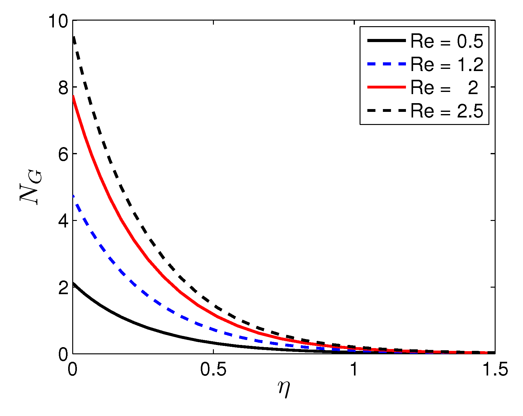
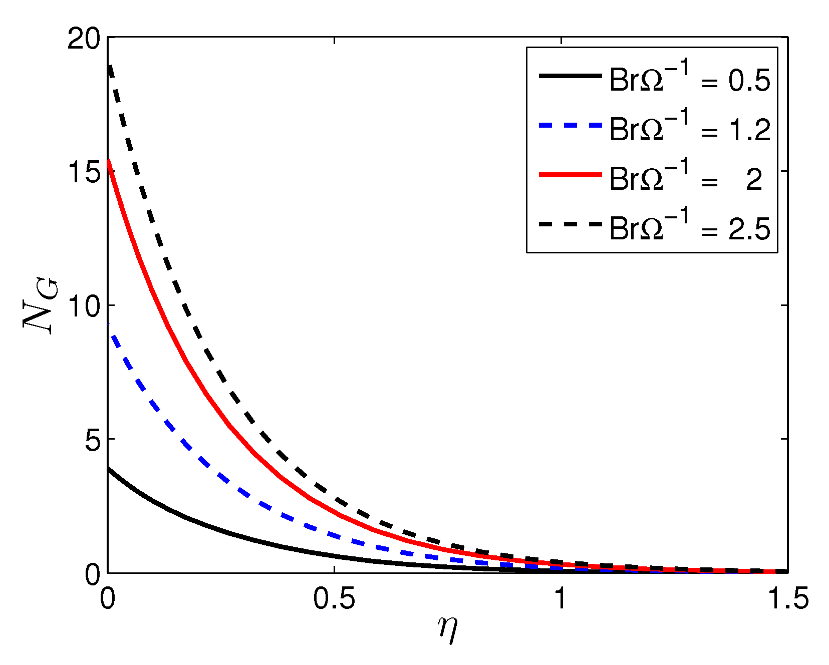
• An increase in the Reynolds number and the Brinkman number corresponds to a significant increase in the entropy generation number. Therefore, it can be ascertained that the entropy generation number is highly affected by viscous dissipation when the nanofluid flow has a large Reynolds number.
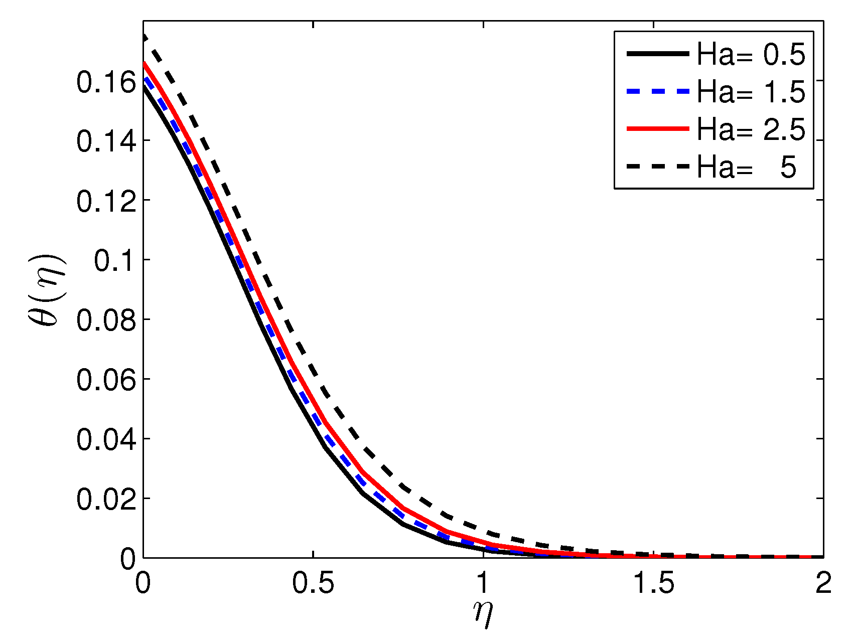
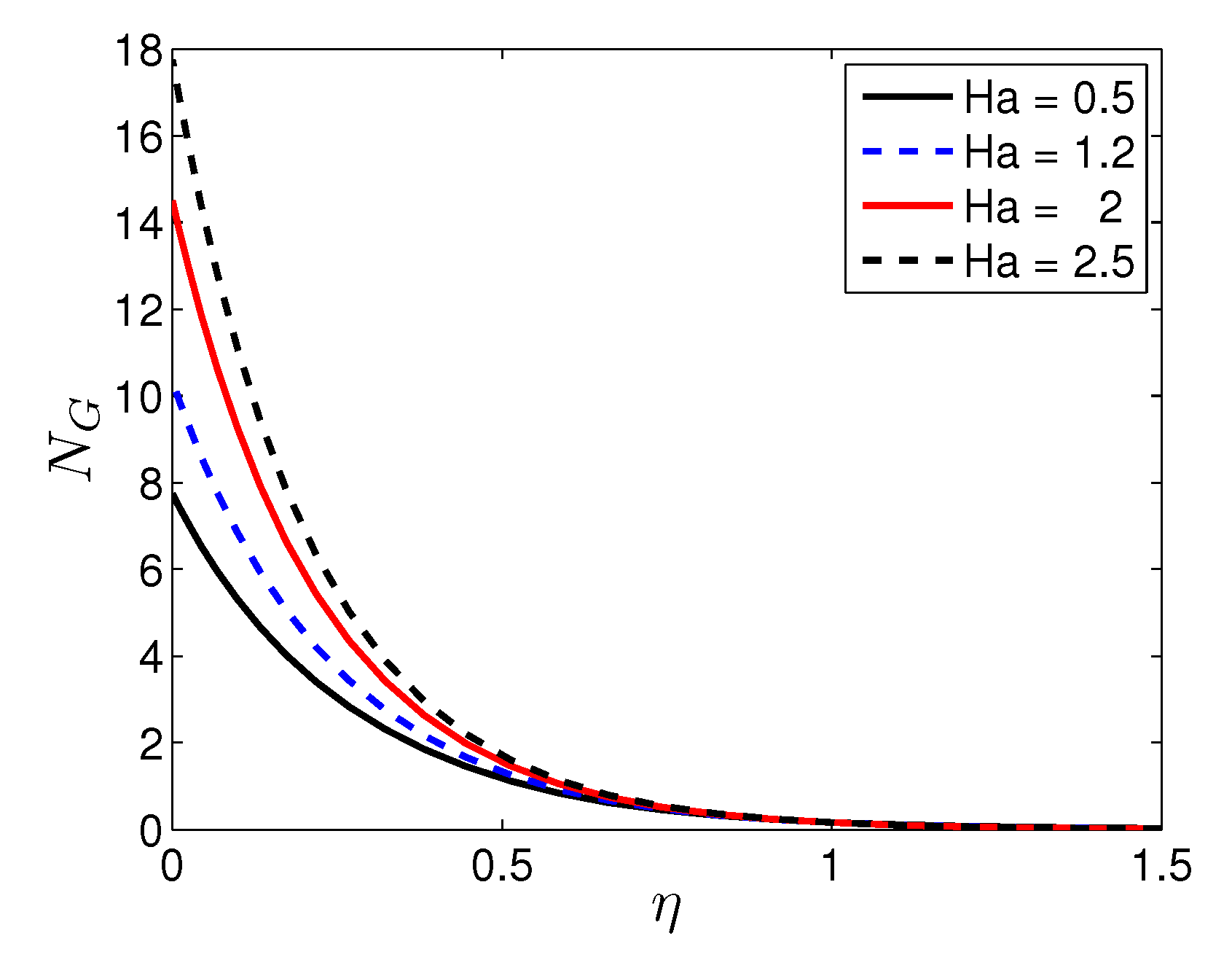
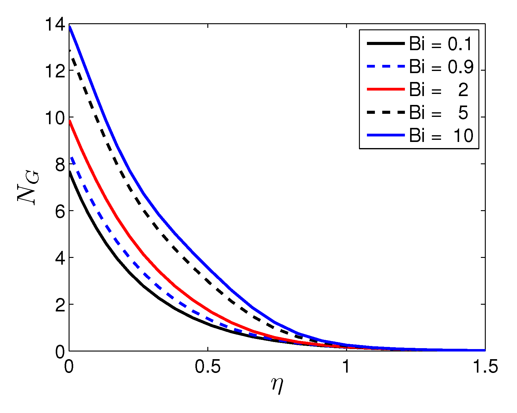
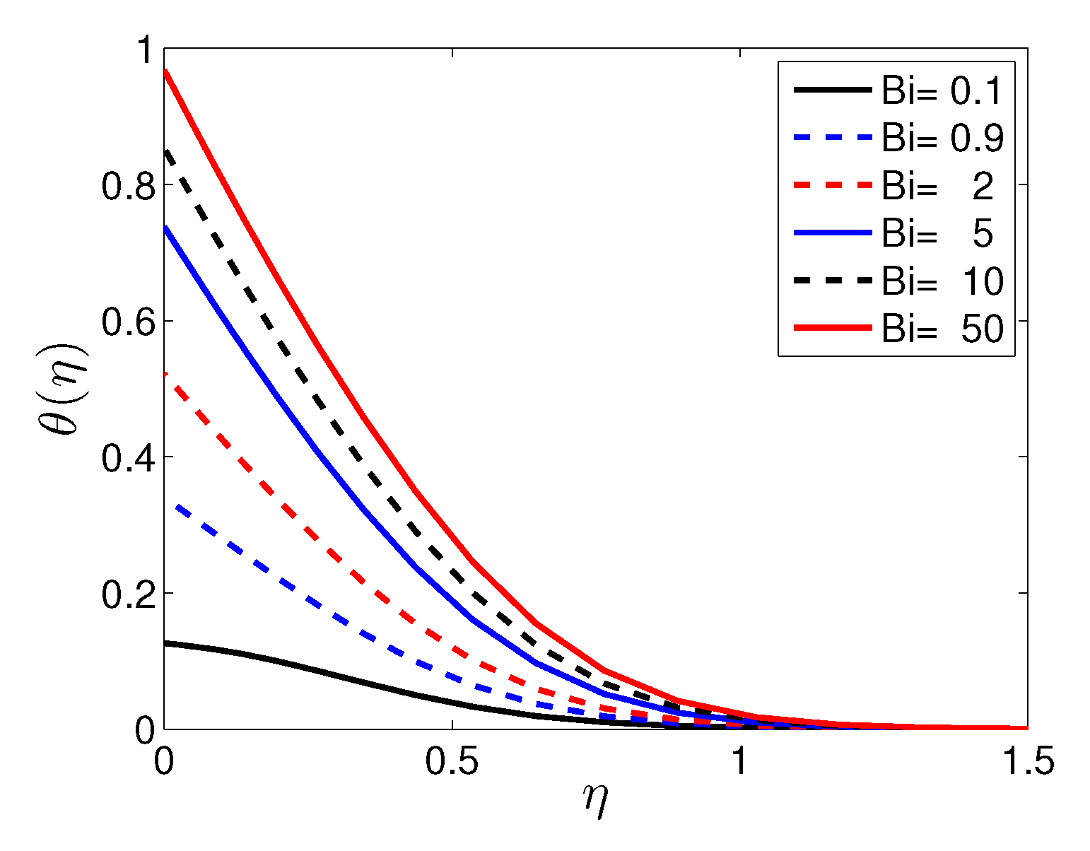
• An increase in the Biot and Hartmann numbers corresponds to a significant increase in the entropy generation number in the vicinity of the sheet surface. The significance of the Biot and Hartmann numbers gradually fades with distance from the sheet.
• The entropy generation rate can be minimized by controlling the physical parameters.
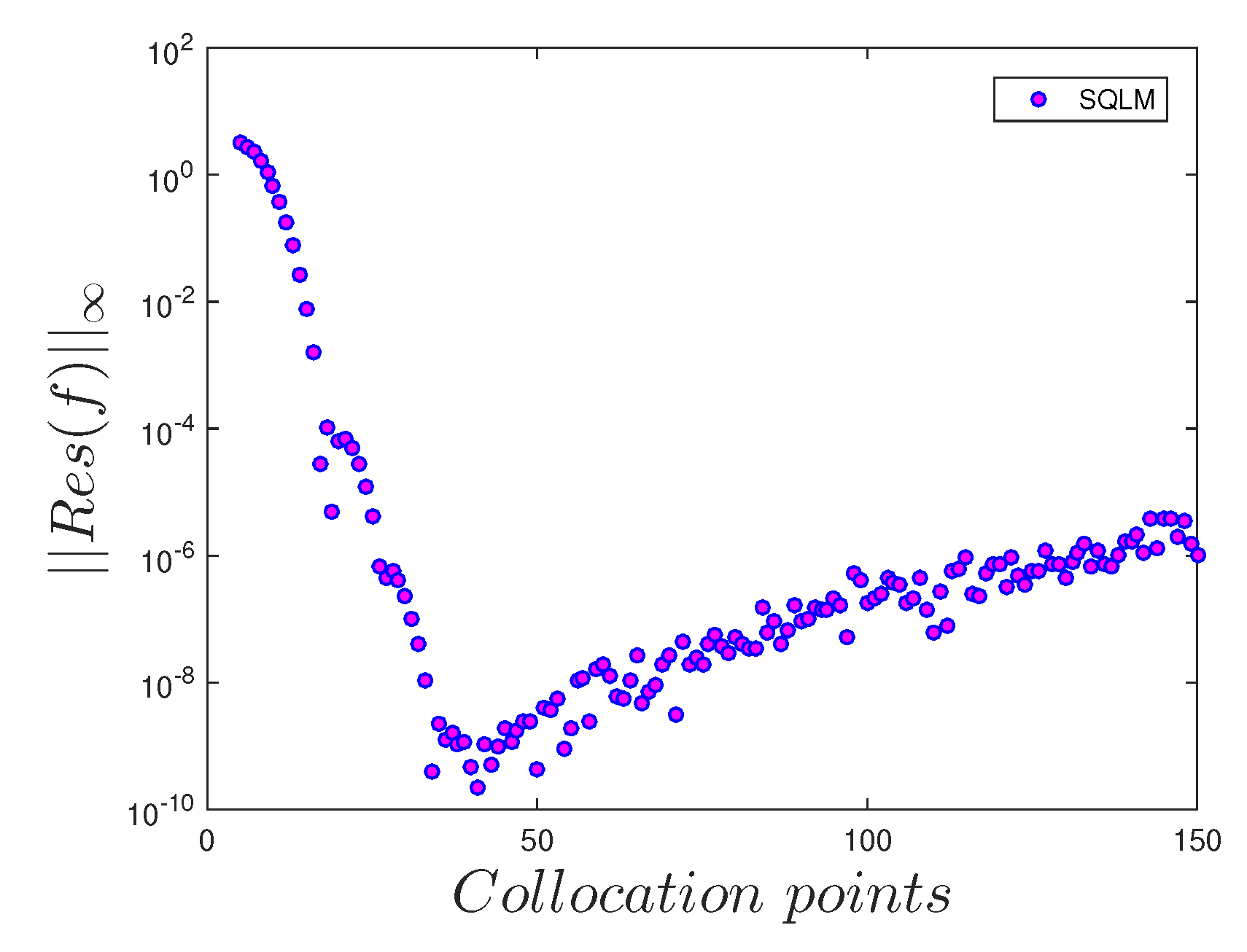
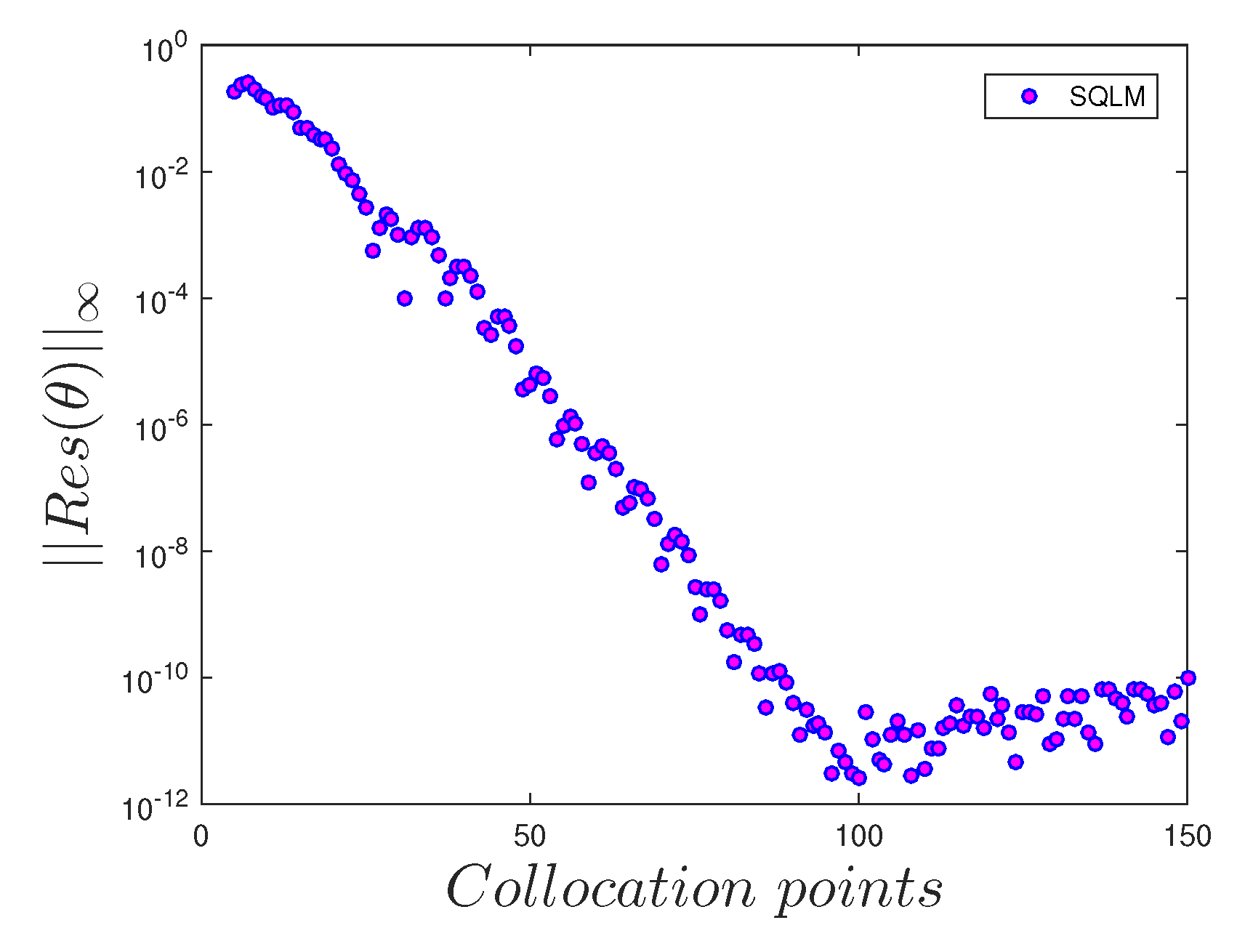
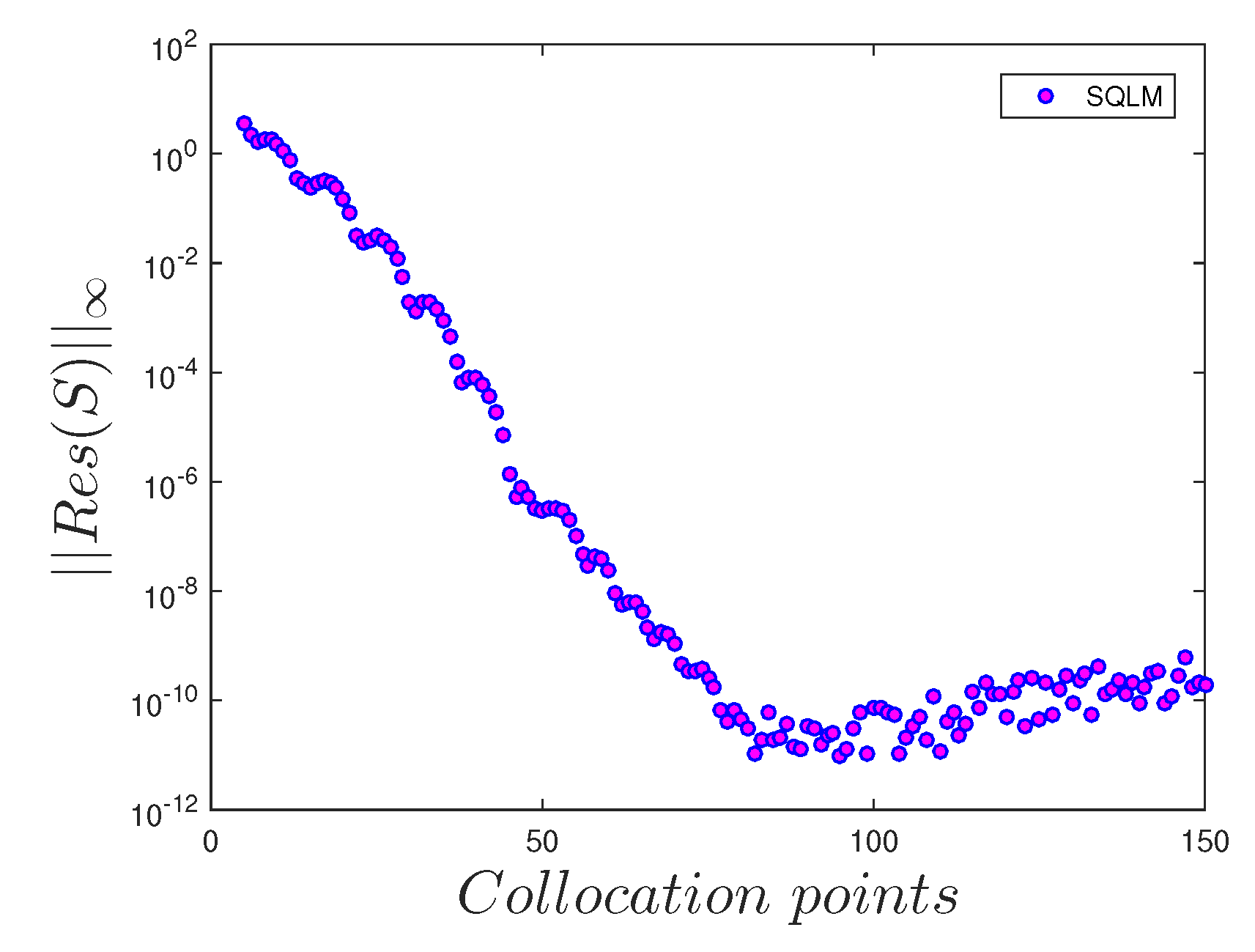
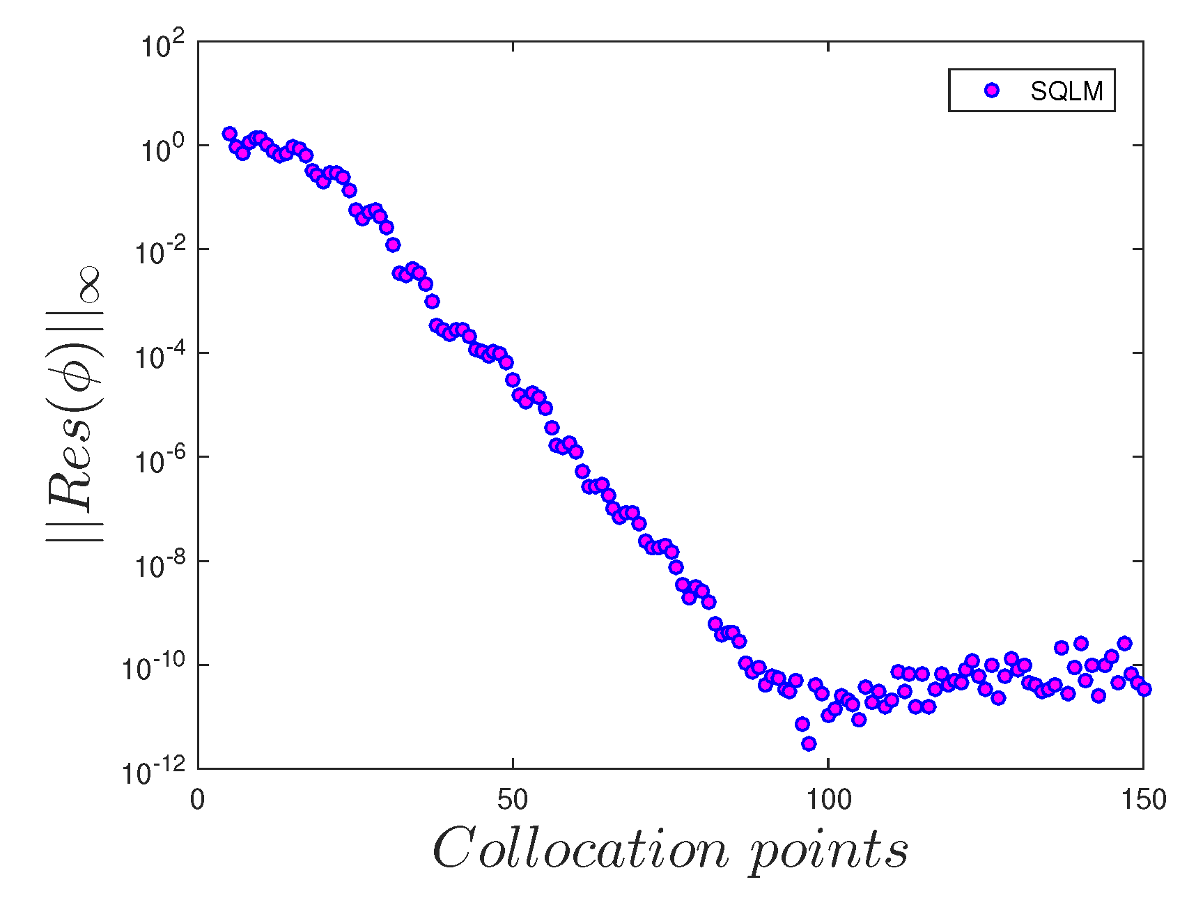
• The number of collocation points has a significant influence on the accuracy of the solutions.

References

1. Dessie, H.; Kishan, N. Unsteady MHD flow of heat and mass transfer of nanofluids over stretching sheet with a non-uniform heat/source/sink considering viscous dissipation and chemical reaction. Int. J. Eng. Res. Afr. 2015, 14. [Google Scholar] [CrossRef]
2. Chol, S. Enhancing thermal conductivity of fluids with nanoparticles. ASME Publ. FED 1995, 231, 99–106. [Google Scholar]
3. Buongiorno, J. Convective transport in nanofluids. J. Heat Transf. 2006, 128, 240–250. [Google Scholar] [CrossRef]
4. Ahmed, N.; Goswami, J.; Barua, D. Effects of chemical reaction and radiation on an unsteady MHD flow past an accelerated infinite vertical plate with variable temperature and mass transfer. Indian J. Pure Appl. Math. 2013, 44, 443–466. [Google Scholar] [CrossRef]
5. Ahmed, J.; Mahmood, T.; Iqbal, Z.; Shahzad, A.; Ali, R. Axisymmetric flow and heat transfer over an unsteady stretching sheet in power law fluid. J. Mol. Liq. 2016, 221, 386–393. [Google Scholar] [CrossRef]
6. Mohammadiun, H.; Rahimi, A.; Kianifar, A. Axisymmetric stagnation-point flow and heat transfer of a viscous, compressible fluid on a cylinder with constant heat flux. Sci. Iran. 2013, 20, 185–194. [Google Scholar] [CrossRef]
7. Xiao, B.; Yang, Y.; Chen, L. Developing a novel form of thermal conductivity of nanofluids with Brownian motion effect by means of fractal geometry. Powder Technol. 2013, 239, 409–414. [Google Scholar] [CrossRef]
8. Cai, J.; Hu, X.; Xiao, B.; Zhou, Y.; Wei, W. Recent developments on fractal-based approaches to nanofluids and nanoparticle aggregation. Int. J. Heat Mass Transf. 2017, 105, 623–637. [Google Scholar] [CrossRef]
9. Shankar, B.; Yirga, Y. Unsteady heat and mass transfer in MHD flow of nanofluids over stretching sheet with a non-uniform heat source/sink. Int. J. Math. Comput. Sci. Eng. 2013, 7, 1267–1275. [Google Scholar]
10. Shahzad, A.; Ali, R.; Khan, M. On the exact solution for axisymmetric flow and heat transfer over a nonlinear radially stretching sheet. Chin. Phys. Lett. 2012, 29, 084705. [Google Scholar] [CrossRef]
11. Ahmad, S.; Ashraf, M.; Syed, K. Effects of thermal radiation on MHD axisymmetric stagnation point flow and heat transfer of a micropolar fluid over a shrinking sheet. World Appl. Sci. J. 2011, 15, 835–848. [Google Scholar]
12. Mabood, F.; Shafiq, A.; Hayat, T.; Abelman, S. Radiation effects on stagnation point flow with melting heat transfer and second order slip. Results Phys. 2017, 7, 31–42. [Google Scholar] [CrossRef]
13. Prasad, K.; Vaidya, H.; Vajravelu, K.; Datti, P.; Umesh, V. Axisymmetric mixed convective MHD flow over a slender cylinder in the presence of chemically reaction. Int. J. Appl. Mech. Eng. 2016, 21, 121–141. [Google Scholar] [CrossRef]
14. Sarada, K.; Shanker, B. The effect of chemical reaction on an unsteady MHD free convection flow past an infinite vertical porous plate with variable suction. Int. J. Eng. Mod. Res. 2013, 3, 725–735. [Google Scholar]
15. Hunegnaw, A.; Kishan, N. Unsteady MHD heat and mass transfer flow over stretching sheet in porous medium with variable properties considering viscous dissipation and chemical reaction. Am. Chem. Sci. J. 2014, 4, 901–917. [Google Scholar] [CrossRef]
16. Barik, R. Heat and Mass Transfer Effects on Unsteady MHD Flow through an Accelerated Isothermal Vertical Plate Embedded in Porous Medium in the Presence of Heat Source and Chemical Reaction. Eur. J. Adv. Eng. Technol. 2016, 3, 56–61. [Google Scholar]
17. Bejan, A. Entropy Generation Minimization: The Method of Thermodynamic Optimization of Finite-Size Systems and Finite-Time Processes; CRC Press: Boca Raton, FL, USA, 1995. [Google Scholar]
18. Qing, J.; Bhatti, M.M.; Abbas, M.A.; Rashidi, M.M.; Ali, M.E.S. Entropy generation on MHD Casson nanofluid flow over a porous stretching/shrinking surface. Entropy 2016, 18, 123. [Google Scholar] [CrossRef]
19. Rashidi, M.M.; Bhatti, M.M.; Abbas, M.A.; Ali, M.E.S. Entropy generation on MHD blood flow of nanofluid due to peristaltic waves. Entropy 2016, 18, 117. [Google Scholar] [CrossRef]
20. Bhatti, M.M.; Abbas, T.; Rashidi, M.M.; Ali, M.E.S.; Yang, Z. Entropy generation on MHD eyring—Powell nanofluid through a permeable stretching surface. Entropy 2016, 18, 224. [Google Scholar] [CrossRef]
21. Rashidi, M.; Mohammadi, F.; Abbasbandy, S.; Alhuthali, M. Entropy generation analysis for stagnation point flow in a porous medium over a permeable stretching surface. J. Appl. Fluid Mech. 2015, 8, 753–765. [Google Scholar] [CrossRef]
22. Bhatti, M.M.; Abbas, T.; Rashidi, M.M.; Ali, M.E.S. Numerical simulation of entropy generation with thermal radiation on MHD Carreau nanofluid towards a shrinking sheet. Entropy 2016, 18, 200. [Google Scholar] [CrossRef]
23. Freidoonimehr, N.; Rahimi, A.B. Comment on “Effects of thermophoresis and Brownian motion on nanofluid heat transfer and entropy generation” by M. Mahmoodi, Sh. Kandelousi, Journal of Molecular Liquids, 211 (2015) 15–24. J. Mol. Liq. 2016, 216, 99–102. [Google Scholar] [CrossRef]
24. Agbaje, T.; Mondal, S.; Makukula, Z.; Motsa, S.; Sibanda, P. A new numerical approach to MHD stagnation point flow and heat transfer towards a stretching sheet. Ain Shams Eng. J. 2016, in press. [Google Scholar] [CrossRef]
25. Kaladhar, K.; Motsa, S.; Srinivasacharya, D. Mixed Convection Flow of Couple Stress Fluid in a Vertical Channel with Radiation and Soret Effects. J. Appl. Fluid Mech. 2016, 9, 43–50. [Google Scholar]
26. Nield, D.; Kuznetsov, A. The onset of convection in a horizontal nanofluid layer of finite depth: A revised model. Int. J. Heat Mass Transf. 2014, 77, 915–918. [Google Scholar] [CrossRef]
27. Mustafa, M.; Khan, J.A.; Hayat, T.; Alsaedi, A. Analytical and numerical solutions for axisymmetric flow of nanofluid due to non-linearly stretching sheet. Int. J. Non Linear Mech. 2015, 71, 22–29. [Google Scholar] [CrossRef]
28. Sajid, M.; Hayat, T.; Asghar, S.; Vajravelu, K. Analytic solution for axisymmetric flow over a nonlinearly stretching sheet. Arch. Appl. Mech. 2008, 78, 127–134. [Google Scholar] [CrossRef]
29. Pal, D. Heat and mass transfer in stagnation-point flow towards a stretching surface in the presence of buoyancy force and thermal radiation. Meccanica 2009, 44, 145–158. [Google Scholar] [CrossRef]
30. Arikoglu, A.; Ozkol, I.; Komurgoz, G. Effect of slip on entropy generation in a single rotating disk in MHD flow. Appl. Energy 2008, 85, 1225–1236. [Google Scholar] [CrossRef]
31. Bellman, R.E.; Kalaba, R.E. Quasilinearization and Nonlinear Boundary-Value Problems; RAND Corporation: New York, NY, USA, 1965. [Google Scholar]
32. Canuto, C.; Hussaini, M.Y.; Quarteroni, A.M.; Thomas, A., Jr. Spectral Methods in Fluid Dynamics; Springer: Berlin/Heidelberg, Germany, 2012. [Google Scholar]
33. Trefethen, L.N. Spectral Methods in MATLAB; SIAM: Oxford, UK, 2000. [Google Scholar]
34. Motsa, S.; Sibanda, P.; Shateyi, S. On a new quasi-linearization method for systems of nonlinear boundary value problems. Math. Methods Appl. Sci. 2011, 34, 1406–1413. [Google Scholar] [CrossRef]
35. Rashidi, M.; Abelman, S.; Mehr, N.F. Entropy generation in steady MHD flow due to a rotating porous disk in a nanofluid. Int. J. Heat Mass Transf. 2013, 62, 515–525. [Google Scholar] [CrossRef]
Figure 1. Physical configuration and coordinate system.
Entropy 19 00168 g001
Figure 2. Effects of the number of collocation points number on the residual error of the velocity profile | | R e s ( f ) | | when n = 3 , A = 0 . 3 , P r = 7 , H a = 0 . 5 , N r = 0 . 2 , N b = 0 . 5 , N t = 0 . 5 , N d = 0 . 02 , L d = 0 . 02 , S c = 7 , R 0 = 0 . 3 , B i = 0 . 2 .
Entropy 19 00168 g002
Figure 3. Effects of the number of collocation points number on the residual error of the temperature profile | | R e s ( θ ) | | when n = 3 , A = 0 . 3 , P r = 7 , H a = 0 . 5 , N r = 0 . 2 , N b = 0 . 5 , N t = 0 . 5 , N d = 0 . 02 , L d = 0 . 02 , S c = 7 , R 0 = 0 . 3 , B i = 0 . 2 .
Entropy 19 00168 g003
Figure 4. Effects of the number of collocation points number on the residual error of the solute concentration profile | | R e s ( S ) | | when n = 3 , A = 0 . 3 , P r = 7 , H a = 0 . 5 , N r = 0 . 2 , N b = 0 . 5 , N t = 0 . 5 , N d = 0 . 02 , L d = 0 . 02 , S c = 7 , R 0 = 0 . 3 , B i = 0 . 2 .
Entropy 19 00168 g004
Figure 5. Effects of the number of collocation points number on the residual error of the nanoparticle concentration profile | | R e s ( ϕ ) | | when n = 3 , A = 0 . 3 , P r = 7 , H a = 0 . 5 , N r = 0 . 2 , N b = 0 . 5 , N t = 0 . 5 , N d = 0 . 02 , L d = 0 . 02 , S c = 7 , R 0 = 0 . 3 , B i = 0 . 2 .
Entropy 19 00168 g005
Figure 6. Effects of the stretching parameter n on f ( η ) when A = 0 . 3 , H a = 0 . 5 , N r = 0 . 2 , P r = 7 , N b = 0 . 5 , N t = 0 . 5 , N d = 0 . 02 , S c = 7 , R 0 = 0 . 3 , L d = 0 . 02 , B i = 0 . 2 .
Entropy 19 00168 g006
Figure 7. Effects of the stretching parameter n on θ ( η ) where A = 0 . 3 , H a = 0 . 5 , N r = 0 . 2 , P r = 10 , N b = 0 . 5 , N t = 0 . 5 , N d = 0 . 02 , S c = 7 , R 0 = 0 . 3 , L d = 0 . 02 , B i = 0 . 2 .
Entropy 19 00168 g007
Figure 8. Effects of the stretching parameter n on S ( η ) for A = 0 . 3 , H a = 0 . 5 , N r = 0 . 2 , P r = 7 , N b = 0 . 5 , N t = 0 . 5 , N d = 0 . 02 , S c = 7 , R 0 = 0 . 3 , L d = 0 . 02 , B i = 0 . 2 .
Entropy 19 00168 g008
Figure 9. Effects of the unsteadiness parameter (A) on θ ( η ) for n = 3 , H a = 0 . 5 , N r = 0 . 2 , P r = 7 , N b = 0 . 5 , N t = 0 . 5 , N d = 0 . 02 , S c = 7 , R 0 = 0 . 3 , L d = 0 . 02 , B i = 0 . 2 .
Entropy 19 00168 g009
Figure 10. Effects of the unsteadiness parameter (A) on S ( η ) when n = 3 , H a = 0 . 5 , N r = 0 . 2 , P r = 7 , N b = 0 . 5 , N t = 0 . 5 , N d = 0 . 02 , S c = 7 , R 0 = 0 . 3 , L d = 0 . 02 , B i = 0 . 2 .
Entropy 19 00168 g010
Figure 11. Effects of the Hartmann number ( H a ) on f ( η ) for n = 3 , A = 0 . 3 , N r = 0 . 2 , P r = 7 , N b = 0 . 5 , N t = 0 . 5 , N d = 0 . 02 , S c = 7 , R 0 = 0 . 3 , L d = 0 . 02 , B i = 0 . 2 .
Entropy 19 00168 g011
Figure 12. Effects of the Hartmann number ( H a ) on θ ( η ) when n = 3 , A = 0 . 3 , N r = 0 . 2 , P r = 7 , N b = 0 . 5 , N t = 0 . 5 , N d = 0 . 02 , S c = 7 , R 0 = 0 . 3 , L d = 0 . 02 , B i = 0 . 2 .
Entropy 19 00168 g012
Figure 13. Effects of the thermal radiation parameter ( N r ) on θ ( η ) where n = 3 , A = 0 . 3 , H a = 0 . 5 , P r = 7 , N b = 0 . 5 , N t = 0 . 5 , N d = 0 . 02 , S c = 7 , R 0 = 0 . 3 , L d = 0 . 02 , B i = 0 . 2 .
Entropy 19 00168 g013
Figure 14. Effects of the Prandtl number ( P r ) on θ ( η ) for n = 3 , A = 0 . 3 , H a = 0 . 5 , N r = 0 . 2 , N b = 0 . 5 , N t = 0 . 5 , N d = 0 . 02 , S c = 7 , R 0 = 0 . 3 , L d = 0 . 02 , β i = 0 . 2 .
Entropy 19 00168 g014
Figure 15. Effects of the thermophoresis parameter ( N t ) on θ ( η ) for n = 3 , A = 0 . 3 , H a = 0 . 5 , N r = 0 . 2 , P r = 7 , N b = 0 . 5 , N d = 0 . 02 , S c = 7 , R 0 = 0 . 3 , L d = 0 . 02 , B i = 0 . 2 .
Entropy 19 00168 g015
Figure 16. Effects of the Schmidt number ( S c ) on S ( η ) for n = 3 , A = 0 . 3 , H a = 0 . 5 , N r = 0 . 2 , P r = 7 , N b = 0 . 5 , N t = 0 . 5 , R 0 = 0 . 3 , B i = 0 . 2 .
Entropy 19 00168 g016
Figure 17. Effects of the Biot number ( B i ) on θ ( η ) for n = 3 , A = 0 . 3 , H a = 0 . 5 , N r = 0 . 2 , P r = 7 , N b = 0 . 5 , N t = 0 . 5 , N d = 0 . 02 , S c = 7 , R 0 = 0 . 3 , L d = 0 . 02 .
Entropy 19 00168 g017
Figure 18. Effects of the stretching parameter (n) on ϕ ( η ) when A = 0 . 3 , H a = 0 . 5 , N r = 0 . 2 , P r = 7 , N b = 0 . 5 , N t = 0 . 5 , N d = 0 . 02 , S c = 7 , R 0 = 0 . 3 , L d = 0 . 02 , B i = 0 . 2 .
Entropy 19 00168 g018
Figure 19. Effects of the unsteadiness parameter (A) on ϕ ( η ) for n = 3 , H a = 0 . 5 , N r = 0 . 2 , P r = 7 , N b = 0 . 5 , N t = 0 . 5 , N d = 0 . 02 , S c = 7 , R 0 = 0 . 3 , L d = 0 . 02 , B i = 0 . 2 .
Entropy 19 00168 g019
Figure 20. Effects of the thermophoresis parameter ( N t ) on ϕ ( η ) for n = 3 , A = 0 . 3 , H a = 0 . 5 , N r = 0 . 2 , P r = 7 , N b = 0 . 5 , N d = 0 . 02 , S c = 7 , R 0 = 0 . 3 , L d = 0 . 02 , B i = 0 . 2 .
Entropy 19 00168 g020
Figure 21. Effects of the Brownian motion parameter ( N b ) on ϕ ( η ) when n = 3 , A = 0 . 3 , H a = 0 . 5 , N r = 0 . 2 , P r = 7 , N t = 0 . 5 , N d = 0 . 02 , S c = 7 , R 0 = 0 . 3 , L d = 0 . 02 , B i = 0 . 2 .
Entropy 19 00168 g021
Figure 22. Effects of the Schmidt number ( S c ) on ϕ ( η ) for n = 3 , A = 0 . 3 , H a = 0 . 5 , N r = 0 . 2 , P r = 7 , N b = 0 . 5 , N t = 0 . 5 , R 0 = 0 . 3 , B i = 0 . 2 .
Entropy 19 00168 g022
Figure 23. Effects of the Reynolds number R e on the entropy generation number N G when N r = 0 . 2 , B r = 1 , Ω = 1 , H a = 0 . 5 and Σ = 0 . 5 .
Entropy 19 00168 g023
Figure 24. Effects of Brinkman number B r on the entropy generation number N G when R e = 2 , N r = 0 . 2 , Ω = 1 , H a = 0 . 5 and Σ = 0 . 5 .
Entropy 19 00168 g024
Figure 25. Effects of Hartmann number H a on the entropy generation number N G when R e = 2 , N r = 0 . 2 , B r = 1 , Ω = 1 and Σ = 0 . 5 .
Entropy 19 00168 g025
Figure 26. Effects of the Brinkman group parameter B r Ω 1 on the entropy generation number N G when R e = 2 , N r = 0 . 2 , B r = 1 and Σ = 0 . 5 .
Entropy 19 00168 g026
Figure 27. Effects of Biot number B i on the entropy generation number N G when R e = 2 , N r = 0 . 2 , B r = 1 , H a = 0 . 5 , Ω = 1 and Σ = 0 . 5 .
Entropy 19 00168 g027
Figure 28. Effect of the magnetic field H a and the stretching sheet parameter n on the skin friction f ( 0 ) when A = 0 . 3 , P r = 7 , N r = 0 . 2 , N b = 0 . 5 , N t = 0 . 5 , N d = 0 . 02 , L d = 0 . 02 , S c = 7 , R 0 = 0 . 3 , B i = 0 . 2 .
Entropy 19 00168 g028
Figure 29. Effect of the thermophoresis number ( N t ) and the stretching sheet parameter (n) on the Nusselt number ( θ ( 0 ) ) when A = 0 . 3 , H a = 0 . 5 , P r = 7 , N r = 0 . 2 , N b = 0 . 5 , N d = 0 . 02 , L d = 0 . 02 , S c = 7 , R 0 = 0 . 3 , B i = 0 . 2 .
Entropy 19 00168 g029
Figure 30. Effect of the Schmidt number S c and the stretching sheet parameter n on the Sherwood number S ( 0 ) when A = 0 . 3 , H a = 0 . 5 , P r = 7 , N r = 0 . 2 , N b = 0 . 5 , N d = 0 . 02 , L d = 0 . 02 , N t = 0 . 5 , R 0 = 0 . 3 , B i = 0 . 2 .
Entropy 19 00168 g030
Figure 31. Effect of the Prandtl number R e and the thermal radiation parameter N r on the Nusselt number θ ( 0 ) when n = 3 , A = 0 . 3 , H a = 0 . 5 , S c = 7 , N b = 0 . 5 , N d = 0 . 02 , L d = 0 . 02 , N t = 0 . 5 , R 0 = 0 . 3 , B i = 0 . 2 .
Entropy 19 00168 g031