
LSTM-CRF for Drug-Named Entity Recognition


School of Computer Science and Technology, Harbin Institute of Technology, 92 West Dazhi Street, Harbin 150001, China
*
Author to whom correspondence should be addressed.
Entropy 2017, 19(6), 283; https://doi.org/10.3390/e19060283
Submission received: 1 April 2017
/
Revised: 9 June 2017
/
Accepted: 9 June 2017
/
Published: 17 June 2017
(This article belongs to the Section Information Theory, Probability and Statistics)
Abstract
:Drug-Named Entity Recognition (DNER) for biomedical literature is a fundamental facilitator of Information Extraction. For this reason, the DDIExtraction2011 (DDI2011) and DDIExtraction2013 (DDI2013) challenge introduced one task aiming at recognition of drug names. State-of-the-art DNER approaches heavily rely on hand-engineered features and domain-specific knowledge which are difficult to collect and define. Therefore, we offer an automatic exploring words and characters level features approach: a recurrent neural network using bidirectional long short-term memory (LSTM) with Conditional Random Fields decoding (LSTM-CRF). Two kinds of word representations are used in this work: word embedding, which is trained from a large amount of text, and character-based representation, which can capture orthographic feature of words. Experimental results on the DDI2011 and DDI2013 dataset show the effect of the proposed LSTM-CRF method. Our method outperforms the best system in the DDI2013 challenge.
1. Introduction
With the rapid development of life science and technology, biomedical literature has increased exponentially. For example, the biomedical literature repository, MEDLINE, collects over 9.6 billions records and grows at 30–50 million records a year (https://www.ncbi.nlm.nih.gov/guide/literature/). This literature contains vast amounts of potential medical information which could be useful to biomedical research, industrial medicine manufacturing, and so forth.
The first step for extracting potential medical information automatically from the vast amounts of biomedical literature is developing a named entity recognition system. This is a crucial part of some therapeutic relation extraction systems or applications, such as drug-drug interactions [1] and adverse drug reactions [2].
Drug-Named Entity Recognition (DNER) is the job of locating drug entity mentions in unstructured medical texts and classifying their predefined categories. Our research interest in DNER mainly comes from two driving reasons: Firstly, new drugs are rapidly and constantly discovered. Secondly, the naming rule is not strictly followed.
The DNER task is full of challenges due to the following reasons: (1) the limited number of supervised training data; (2) new drug entity names are increasing constantly; (3) the authors of biomedical literature do not always follow proposed standardized name rules or formats. Previous works for DNER usually include two steps: the first is to construct orthographic features or training word embedding [3] and the second is to employ machine learning methods, such as Conditional Random Fields [4], support vector machines [5], maximum entropy [6,7] and so forth. CRF become the best choice for DNER since CRF is one of the most reliable sequence labeling methods, which has shown good performances on different kinds of named entity recognition (NER) tasks. For example, NER application in the newswire domain [8,9]. Researchers also explore biomedical knowledge resources, such as constructing a new drug dictionary [10,11]. In recent years, people have been eager to use neural network methods to develop DNER systems [12], which can learn the feature representation from the raw input automatically and avoid costly feature engineering process.
LSTM [13] is suitable for process variable input, and has a long term memory. The detail can be viewed in Section 2.1. Recent LSTM methods make a great success in NLP tasks. Such as NER task [14] and sequence tagging [15]. In our work, we construct a model using a bi-directional LSTMs with a random sequential conditional layer (LSTM-CRF) beyond it inspired by [15]. Entity names are usually composed of multiple tokens, so tag decision for each token is necessary. Considering dependencies across the output label in the DNER task, instead of using softmax function in the output layer of recurrent neural network, we choose CRF to do classification decisions.
Bi-directional LSTM-CRF is an end-to-end solution. It can learn features from a dataset automatically during the training process. So it is not necessary to deign hand-crafted features and biomedical knowledge resources are also not prerequisite. Bi-directional LSTMs learn to how to identify named entities based on sentence level information and take the combination of word embedding and character embedding as inputs. The outputs of the bi-directional LSTMs will be fed into the CRF layer. The CRF layer will output the label sequence with the maximum score calculated by the Equation (14).
We observe that sole dependence on word embedding will ignore explicit character level features like the prefix and suffix [16]. However, some character sequences in words can show orthographic construction features that could be useful indicators for DNER, particularly when word embedding is poorly trained. In order to deal with these issues, we combine word embedding features with character level information as final word representations in the LSTM-CRF models. Experimental results in DDIExtraction2011 and DDIExtraction2013 dataset show that the proposed method can achieve comparable performance with the state-of-the-art performance in original challenge reports without any constructed drug dictionary or any hand-built features.
2. LSTM-CRF Model
2.1. LSTM
Recurrent neural networks (RNNs) [17,18,19] is a family of neural networks, RNNs has a high-dimensional hidden state with non-linear dynamics that encourage RNNs to take advantage of previous information. It is specialized in processing a sequence of values (, , ... , ), then computing a corresponding hidden states sequence (, , ..., ) and outputs (, , ..., ). We develop the forward propagation formula beginning with a specification of the initial state . Each step time variable i ranges from 1 to n, and we apply the update equations as follows:
where the parameters b and c are bias vectors, along with three parameters , , respectively for input-to-hidden weight matrix, hidden-to-hidden (or recurrent) weight matrix, hidden-to-output weight matrix.
In principle, RNNs is a powerful and simple model, and one can readily compute the gradients of the RNNs with back-propagation through time (BPTT), and can flow for long durations without sequence-based specialization. In fact, they fail to result in an effective effect due to the difficulty of training with BPTT and the vanishing and exploding gradient problems, refer to the paper [20] for detail.
So far, gated RNNs are the most effective sequence models in practical applications, including LSTM [13]. LSTM can address the vanishing and exploding gradient problems by adding extra memory cell inherent in RNNs. The fundamental idea of proposing self-loops to yield paths where the gradient can learn long dependencies are a core contribution of the initial LSTM model. There is an internal recurrence (a self-loop) in the LSTM cell, each cell has a system of gating units that control the flow of information; the self-loop weight is controlled by forget gate unit (cell i at time step t), which ranges from 0 to 1, shown in Equation (5).
where is the current input vector and is the hidden state vector, including the outputs of all past cells, and , , are respectively the biases, input weights and recurrent weights for the forget gate units. The state unit update in Equation (6)
where the input gate unit has the similar equation with different parameters, described in Equation (7):
Finally, we can get output of the cell through the output gate , which uses a sigmoid unit for gating, shown in the following two equations.
We use the bi-directional LSTM [21] instead of a single forward network. For instance, given a sentence (, , ..., ), for each word , we apply LSTM to compute the representation of left context for the sentence, and vice versa, then we can get representation of the right context by reversing the sentence. Concatenation of the left and right context representations gives the final representations [, ] of a word, and this representation is very useful for the tagging system.
2.2. CRF Model
We use the final representations [, ] as features to make tagging decisions independently, which is extremely effective for each output [15]. However, classification independently is insufficient because the output has strong dependencies, such as our task: DNER. When we imposed a tag for each word, the sequences of tags contain their own limitation, for example, logically the tag “I-BRAND” cannot follow behind the tag “B-DRUG”. So the DNER tasks fail to model by the independent decisions. CRF is an undirected graphical models, which focus on the sentence level instead of individual positions.
Consider an input sequence Z = {, , ..., } where is the input vector of the i-th word, and y = {, , ..., } is the corresponding label sequences for sentence Z. We use P as the matrix of scores which is outputted from bi-directional LSTM, P is of size , where k is the number of distinct tags, is the core of the j-th tag of the i-th character, its score defined by Equation (10):
where A is a matrix of transition scores, represents the score of a transition from the tag i to tag j. We use and at the start and end tags of a sentence, then we add to the set of possible tags. So A is a square matrix of size .
We denoted the as the set of possible label sequences for z. The probabilistic model for the sequence of CRF gives a series of probability with all possible label sequences y under the given z as the following equations:
where and respectively are the weight vector or matrix and bias for the label pair .
During the CRF training, we optimize the use of log-probability of the correct label sequence. For a set , the logarithm of the likelihood showed in Equation (13):
During the training, CRF would regulate the parameters to maximize the logarithm of the likelihood and search for label under the maximum conditional probability shown in Equation (14):
For a sequence CRF model, training and decoding can be solved efficiently by the Viterbi algorithm.
2.3. LSTM-CRF
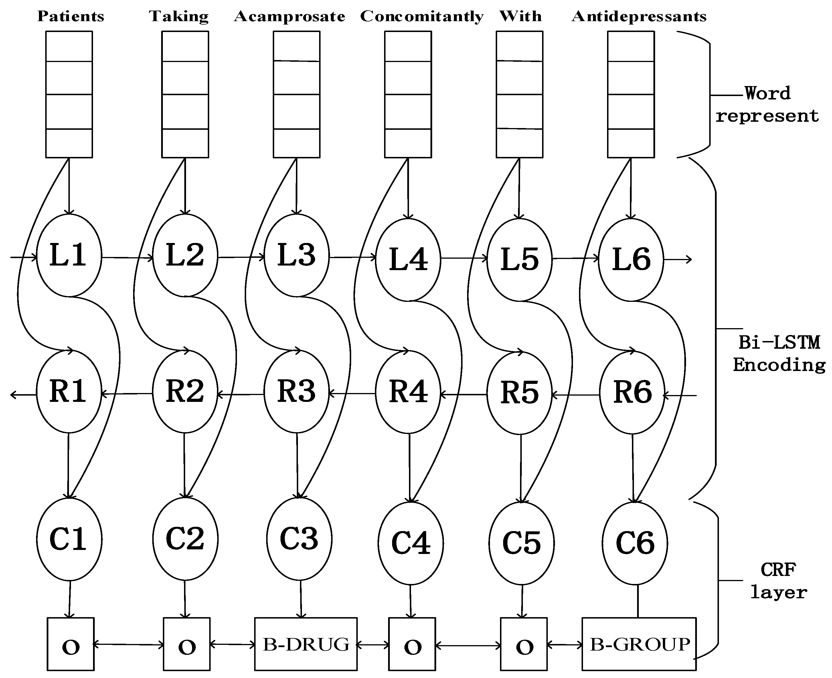
The neural network architecture is shown in Figure 1. The top strip-type stands for the observed variables, the oval represent deterministic functions of their outputs, and the bottom rectangle is the label. As describes in Section 2.2, the denotes the input of word representation at sentence level, and is the corresponding label. The process of producing word representation will be described in Section 2.4.3. The sequence of word representation is regarded as inputs to a bi-directional LSTM, and its output results from the right and left context (in Figure 1, Li is the left context and Ri is the right context for word i; Ci is the concatenation of Li and Ri) for each word in a sentence, as Section 2.1 presented. The output representation from bi-directional LSTM fed onto a CRF layer, the size of representation and its labels are equivalent. In order to consider the neighboring labels, instead of the softmax, we chose CRF as a decision function to yield final label sequence.
2.4. Embedding and Network Training
In this section, we provide the detail process of our neural network training. We apply the Theano library [22] to implement our system.
We train our network architecture with the back-propagation algorithm to update the parameters for each training example with stochastic gradient descent (SGD). Our epoch size is set to 100. In each epoch, we divide all the training data into batches, then process one batch at a time. The batch size decides the number of sentences and our batch size is 100. In each batch, we firstly get the output scores from the bi-directional LSTM for all labels. Then we put the output scores into CRF model, and we can get the gradient of outputs and the state transition edges. From this, we can back propagate the error from output to input, which contains the backward propagation for bi-directional states of LSTM. Finally, we update the parameters including the which represents the score of a transition from the tag i to tag j, and some other parameters such as , , from LSTM.
2.4.1. Parameters Initialization
Word embedding: It is more efficient to use word embeddings than randomly initialized directly [23], we employed existing word embedding to initialize our lookup table. The word embedding are trained on entire English Wikipedia [24]. and produced by skip-n-gram [25] and Word2Vec [26], which account for word order. These embedding are fine-tuned during training.
Character embedding: character level evidence for a name is derived from orthographic feature. We apply character level features instead of hand-craft prefix and suffix construction features of words. It has been found that building character embedding is beneficial to learning representations in specific domains, and is always useful for morphologically rich languages and dealing with the out-of-vocabulary problem, such as part-of-speech tagging [25].
We collect all characters forming a character set which contains 26 upper and lower case letters (in our work, changing all letters to their lowercase), 10 numbers and 33 punctuation. The details are shown in Table 1.
We initialized a character lookup table randomly with values ranging from = to = 1.0 for the output of 50 dimensions embedding, which drew by a uniform distribution.
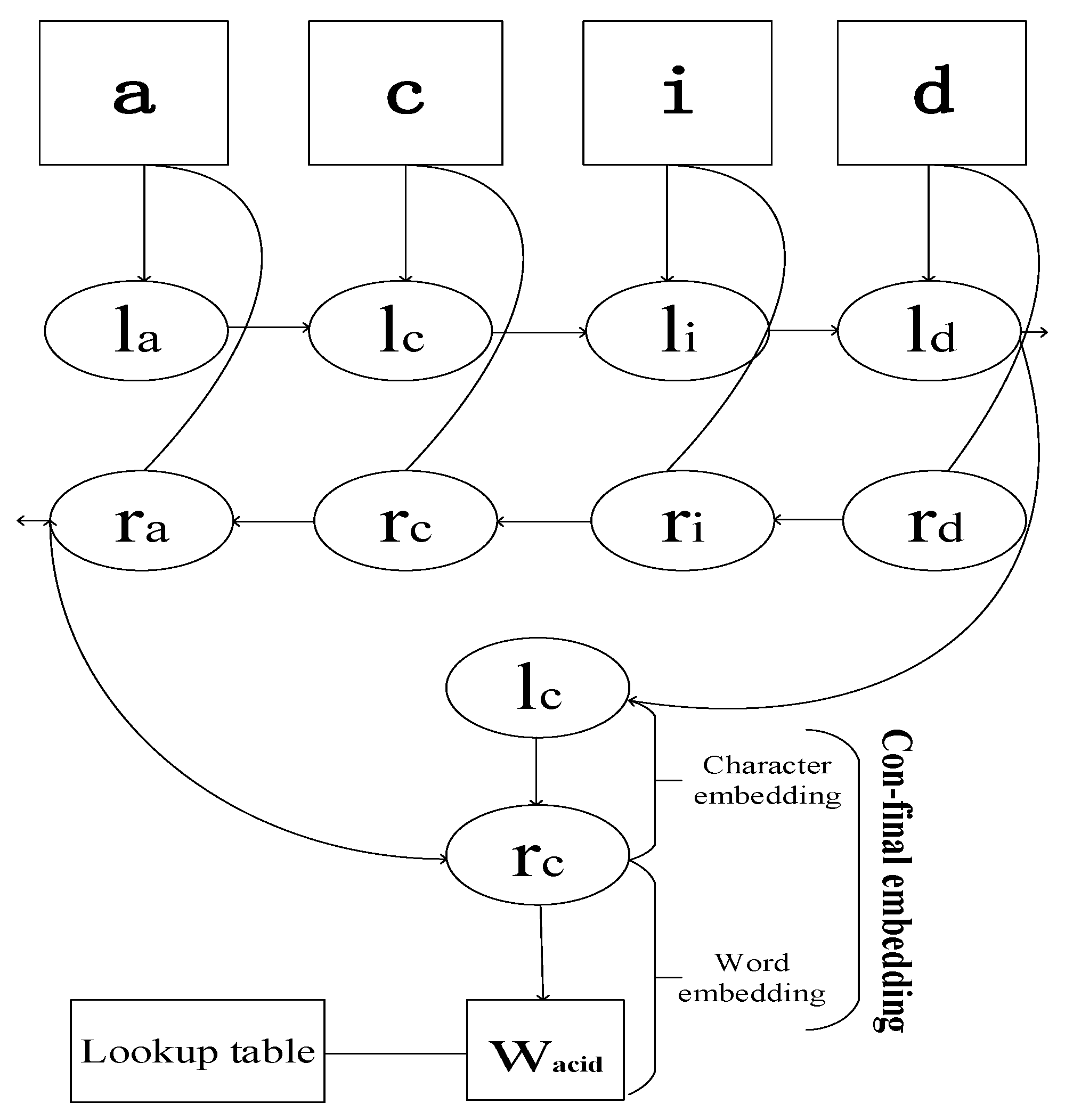
Finally, our word representation is obtained by the architecture, which is shown in Figure 2. We construct character embedding with supervised training method using NER labels during the training process. Character level embedding for a word is given by direct and reverse order to the bi-directional LSTM with dimensions 25 respectively, and the result produces a vector with dimensions 50. Then we concatenated the result with its word embedding. Words out of the lookup table will be replaced as token “UNK“ and be mapped as UNK embedding, which is initialized by random. Refer to the paper [27], if a word is less than two letters we replace it with UNK embedding under a probability ().
2.4.2. Optimization Method
We chose the mini-batch stochastic gradient descent, with a fixed learning rate of 0.01 and a gradient clipping of 5.0 [28], to optimize our parameters. Some similar methods have been applied to improve the performance of SGD, like Adadelta [29], Adam [30] and RMSProp [31]. Unfortunately, among the preliminary experiment [32], none of them could enhance the SGD.
Dropout [33] can mitigate over-fitting. The paper [27] has proved that dropout can be beneficial to the NER task, which can avoid the over-fitting problem. So we apply dropout on the weight vectors directly to mask the final embedding layer before the combinational embedding feed into the bi-directional LSTM. We fix dropout rate at 0.5 as usual, and achieve good performance on our model.
2.4.3. Parameters Adjustment
Our hyper-parameters showed in Table 2. In our experiment, referring to previous work [14,23,34], we set the state size of character for LSTM to 25 respectively for forward and backward, the dimension of character-based representation of words has been set at 50. The dimension of word embedding and word has been set at 100. The dimension of Con-Final Embedding has been set at 150. The dropout rate is 0.5 and initial learning rate is 0.01.
2.5. IOBES Tagging Scheme
Similar to the task of part-of-speech tagging, DNER also aims to assign a label to each word among a sentence. Due to there being some entity names containing more than one token in a sentence, typically, each token is encoded in IOB format (Inside, Outside, Begin), respectively if the token is inside (but not the first token within an entity name), or outside in entity name and the beginning of entity name. Take an example from Figure 1, from the part of a sentence “”, the corresponding label is “––”.
3. Experiments
3.1. Data Sets
In our experiments, we primarily used the DDI2011 challenge corpus from the drug-drug interactions task (http://labda.inf.uc3m.es/DDIExtraction2011/). Refer to Task 9.1: Recognition and classification of drug names (http://www.cs.york.ac.uk/semeval-2013/task9/). For the DDI2011 challenge corpus, we use the NLP package Natural Language Toolkit (https://docs.python.org/2/library/xml.etree.elementtree.html) to parse all the XML format documents, then collect all the train dataset as the training data, and gather all the test dataset as the testing data. Table 3 shows the distribution of the documents, sentences and drugs in the train and test set from DDI2011. The train and test dataset contain 435 and 144 documents, 4267 and 1539 sentences, 11,260 and 3689 drugs respectively [35]. In this corpus, there is only one type with the entity name: drug, so each word in a sentence just be labeled as “B/I-DRUG” or “O”. In our experiment, apart from replacing all digits with zero, we did not do any additional preprocessing on the challenge dataset.
In order to further evaluate our model, we use the dataset from the Recognition and Classification of drug names task of SemEval-2013 (http://www.cs.york.ac.uk/semeval-2013/task9/). This task concerns the named entity extraction of mentions of pharmacological substances in text (https://www.cs.york.ac.uk/semeval-2013/task9/data/uploads/semeval_2013-task-9_1-evaluationmetrics.pdf). Table 4 and Table 5 show the numbers of the annotated entity in the DDI2013 training set and the testing set respectively. The corpus derives from two sources: DrugBank (https://www.drugbank.ca/) and MedLine (https://www.ncbi.nlm.nih.gov/pubmed/?term=meline). There are four general types of entities: Drug, Brand, Group, Drug_n [36]. Where Drug type is denoted as human medicines known as a generic name. The Brand type is characterized by a trade or brand name. Group type annotates groups of drugs. Finally, Drug_n type describes those substances like pesticides or toxins not available for human use.
3.2. Evaluation Metrics
In our experiment, we use precision recall, F1 to evaluate the performance of our system, and we use two of the four evaluation criteria provided by the DDI2013 challenge [36], the Type matching (a tagged drug name is correct only if there is some overlap between it and a gold drug name of the same class) and Strict matching (a tagged drug name is correct only if its boundary and class exactly match with a gold drug name). A detailed description of evaluation is in the document (https://www.cs.york.ac.uk/semeval2013/task9/data/uploads/semeval_2013-task-9_1-evaluation-metrics.pdf). Finally, we use evaluation scripts (https://www.cs.york.ac.uk/semeval-2013/task9/index.php%3Fid=evaluation.html) provided by the shared task organizers to evaluate our system.
3.3. Results
Table 6 displays the results of the experiment, which was performed on the DDI2011 corpus. We can achieve the precision of 93.26%, recall of 91.11% and F1 of 92.04%. Comparing our result with previous best results [37], which were obtained by building a man-made dictionary and using CRF method we find that our precision is lower than the best performance by 1.5%. However, our recall is higher than the best performance by 0.6%. However, when their system just uses CRF method without the dictionary assistant, the performance of our system outperforms their evaluation values.
Table 7 shows all types of the entities and their detailed evaluation. We can observe that our method is efficient in correctly classifying the Drug, Brand and Group types, where it achieves an F1 of over 80% correspondingly. However, our method has a few difficulties in correctly classifying named entities of the Drug_n type, the F1 of 62.83% was achieved. A previous work [38] showed that the Drug_n entity type was demonstrated to be a very difficult type to be classified correctly. According to our analysis, the low percentage of this type in the training dataset (<4%) result in ignoring the difference between this type and a much larger class of Drug or Group type, which would lead to the fact that some of the Drug_n type entities had been changed to human use. So the feature extraction applied to efficient detection of the Drug_n type cannot efficiently reflect the knowledge about drug conform for human use.
In order to further investigate our achievement, we compared our results with other teams’ work on the DDI2013 challenge, Table 8 shows the comparison, it can be found the performance of our work outperforms the WBI which ranks 1st of the original teams in the DDI2013 challenge, improved by the precision of a 6.92% points (from 76.70% to 83.62%), the recall of a 4.81% points (from 73.00% to 77.81%) and the F1 of a 4.46% points (from 74.80% to 79.26%). When compared with LIU, the precision falls by 3.84% points and the F1 falls by 1.62% points, but the recall has achieved an increase of approximately 2.59% points (from 75.22% to 77.81%).
Finally, we try to do a statistical significance test for the results in Table 6 and Table 7. We plan to apply the McNemar’s significance test to decide whether statistically significant difference exists between our runs with others. McNemar’s test is grounded on a goodness-of-fit test, which compares the distribution of counts expected with the counts observed under null hypothesis. The null hypothesis defined as the two runs have the same error state. Unfortunately, all the results of other models are obtained from the corresponding references. Therefore, we cannot obtain the detailed counts for each entity category in each model which are necessary for a statistical significance test. However, according to [36], the results between our methods and others in Table 8 should be significant.
4. Conclusions
In this paper, we discuss the recent advanced neural networks methods that are able to achieve the task of DNER without requiring additional knowledge or hand-crafted features. Inspired by this kind of work, we construct a bi-directional LSTM and CRF architecture. The input vector of the architecture is the concatenation of word embedding and character-level embedding from a sentence, the output of the architecture is a label sequence. Our experiments were conducted on two biomedical literature datasets: the DDI2011 and the DDI2013. The proposed method achieved comparable performances with the state-of-the-art results of both of the datasets.
Acknowledgments
This work is sponsored by the National High Technology Research and Development Program of China (2015AA015405) and National Natural Science Foundation of China (61572151 and 61602131).
Author Contributions
The author Donghuo Zeng’s contributions were literature research, code programming, experimental studies, data acquisition and data analysis. The author Chengjie Sun’s contributions were study design, study concepts, manuscript preparation. The author Lei Lin’s contributions were manuscript editing, manuscript revision and manuscript review. The author Bingquan Liu’s contributions were literature research, statistical analysis and manuscript final version approval.
Conflicts of Interest
The authors declare no conflict of interest.
References
- Segura-Bedmar, I.; Martínez, P.; Pablo-Sánchez, C. Using a shallow linguistic kernel for drug-drug interaction extraction. J. Biomed. Inform. 2011, 44, 789–804. [Google Scholar] [CrossRef]
- Warrer, P.; Hansen, W.; Juhl-Jensen, L.; Aagaard, L. Using text-mining techniques in electronic patient records to identify ADRs from medicine use. Br. J. Clin. Pharmacol. 2012, 73, 674–684. [Google Scholar] [CrossRef]
- Segura-Bedmar, I.; Suárez-Paniagua, V.; Martínez, P. Exploring word embedding for drug name recognition. In Proceedings of the International Workshop on Health Text Mining and Information Analysis, Lisbon, Portugal, 17 September 2015; pp. 64–72. [Google Scholar]
- Li, K.; Ai, W.; Tang, Z.; Zhang, F.; Jiang, L.; Li, K.; Hwang, K. Hadoop recognition of biomedical named entity using conditional random fields. IEEE Trans. Parallel Distrib. Syst. 2015, 26, 3040–3051. [Google Scholar] [CrossRef]
- Kazama, J.; Makino, T.; Ohta, Y.; Tsujii, J. Tuning support vector machines for biomedical named entity recognition. In Proceedings of the ACL Workshop on Natural Language Processing in the Biomedical Domain, Philadelphia, PA, USA, 11 July 2002; pp. 1–8. [Google Scholar]
- Saha, S.K.; Sarkar, S.; Mitra, P. Feature selection techniques for maximum entropy based biomedical named entity recognition. J. Biomed. Inform. 2009, 42, 905–911. [Google Scholar] [CrossRef]
- Lin, Y.; Tsai, T.; Chou, W.; Wu, K.; Sung, T.; Hsu, W. A maximum entropy approach to biomedical named entity recognition. In Proceedings of the 4th International Conference on Data Mining in Bioinformatics, Seattle, WA, USA, 28 June 2004; pp. 56–61. [Google Scholar]
- Finkel, J.R.; Grenager, T.; Manning, C.D. Incorporating non-local information into information extraction systems by Gibbs sampling. In Proceedings of the 43rd Annual Meeting on Association for Computational Linguistics, Ann Arbor, MI, USA, 25–30 June 2005; pp. 363–370. [Google Scholar]
- Tkachenko, M.; Simanovsky, A. Named entity recognition: Exploring features. In Proceedings of the 11th Conference on Natural Language Processing, Vienna, Austria, 19–21 September 2012; pp. 118–127. [Google Scholar]
- Zeng, D.; Sun, C.; Lin, L.; Liu, B. Enlarging drug dictionary with semi-supervised learning for Drug Entity Recognition. In Proceedings of the IEEE International Conference on Bioinformatics and Biomedicine, Shenzhen, China, 15–18 December 2016; pp. 1929–1931. [Google Scholar]
- Eriksson, R.; Jensen, P.B.; Frankild, S.; Jensen, L.J.; Brunak, S. Dictionary construction and identification of possible adverse drug events in Danish clinical narrative text. J. Am. Med. Inform. Assoc. 2013, 20, 947–953. [Google Scholar] [CrossRef]
- Chalapathy, R.; Borzeshi, E.Z.; Piccardi, M. An investigation of recurrent neural architectures for drug name recognition. arXiv, 2016; arXiv:1609.07585. [Google Scholar]
- Hochreiter, S.; Schmidhuber, J. Long short-term memory. Neural Comput. 1997, 9, 1735–1780. [Google Scholar] [CrossRef]
- Hammerton, J. Named entity recognition with long short-term memory. In Proceedings of the 7th conference on Natural language learning, Edmonton, AB, Canada, 31 May–1 June 2003; pp. 172–175. [Google Scholar]
- Huang, Z.; Xu, W.; Yu, K. Bidirectional LSTM-CRF models for sequence tagging. arXiv, 2015; arXiv:1508.01991. [Google Scholar]
- Dos Santos, C.N.; Zadrozny, B. Learning character-level representations for part-of-speech tagging. In Proceedings of the 31st International Conference on Machine Learning, Beijing, China, 21–26 June 2014; pp. 1818–1826. [Google Scholar]
- Rumelhart, D.; Hinton, G.; Williams, R. Learning representations by back-propagating errors. Nature 1986, 323, 533–536. [Google Scholar] [CrossRef]
- Elman, J. Finding structure in time. Cogn. Sci. 1990, 14, 179–211. [Google Scholar] [CrossRef]
- Werbos, P.J. Generalization of backpropagation with application to a recurrent gas market model. Neural Netw. 1998, 1, 339–356. [Google Scholar] [CrossRef]
- Bengio, Y.; Simard, P.; Frasconi, P. Learning long-term dependencies with gradient descent is difficult. IEEE Trans. Neural Netw. 1994, 5, 157–166. [Google Scholar] [CrossRef]
- Graves, A.; Schmidhuber, J. Framewise phoneme classification with bidirectional LSTM networks. In Proceedings of the 2005 International Joint Conference on Neural Networks, Montreal, QC, Canada, 31 July–4 Aug 2005; pp. 2047–2052. [Google Scholar]
- Bergstra, J.; Breuleux, O.; Bastien, F.; Lamblin, P.; Pascanu, R.; Desjardins, G.; Turian, J.; Bengio, Y. Theano: A CPU and GPU math expression compiler. In Proceedings of the Python for Scientific Computing Conference, Austin, TX, USA, 28 June–3 July 2010; pp. 3–10. [Google Scholar]
- Collobert, R.; Weston, J.; Bottou, L.; Karlen, M.; Kavukcuoglu, K.; Kuksa, P.P. Natural language processing (almost) from scratch. J. Mach. Learn. Res. 2011, 12, 2493–2537. [Google Scholar]
- Wikimedia Downloads. Available online: http://download.wikimedia.org (accessed on 11 June 2017).
- Ling, W.; Marujo, T.; Astudillo, F.; Amir, S.; Dyer, C.; Black, A.W.; Trancoso, I. Finding function in form: Compositional character models for open vocabulary word representation. In Proceedings of the Conference on Empirical Methods in Natural Language Processing, Lisbon, Portugal, 17–21 September 2015; pp. 1520–1530. [Google Scholar]
- Mikolov, T.; Chen, K.; Corrado, G.; Dean, J. Efficient estimation of word representations in vector space. arXiv, 2013; arXiv:1301.3781. [Google Scholar]
- Lample, G.; Ballesteros, M.; Subramanian, S.; Kawakami, K.; Dyer, C. Neural architectures for named entity recognition. arXiv, 2016; arXiv:1603.01360. [Google Scholar]
- Pascanu, R.; Mikolov, T.; Bengio, Y. On the difficulty of training recurrent neural networks. arXiv, 2012; arXiv:1211.5063. [Google Scholar]
- Zeiler, M.D. ADADELTA: An adaptive learning rate method. arXiv, 2015; arXiv:1212.5701. [Google Scholar]
- Kingma, D.; Ba, J. Adam: A method for stochastic optimization. arXiv, 2014; arXiv:1412.6980. [Google Scholar]
- Hinton, G.; Srivastava, N.; Swersky, K. RMSProp: Divide the gradient by a running average of its recent magnitude. Available online: http://www.cs.toronto.edu/~tijmen/csc321/slides/lecture_slides_lec6.pdf (accessed on 10 June 2017).
- Ma, X.; Hovy, E.H. End-to-end sequence labeling via bi-directional LSTM-CNNs-CRF. arXiv, 2016; arXiv:1603.01354. [Google Scholar]
- Srivastava, N.; Hinton, G.; Krizhevsky, A.; Sutskever, I.; Salakhutdinov, R. Dropout: A simple way to prevent neural networks from overfitting. J. Mach. Learn. Res. 2014, 15, 1929–1958. [Google Scholar]
- Dos Santos, C.N.; Guimarães, V. Boosting named entity recognition with neural character embeddings. arXiv, 2015; arXiv:1505.05008. [Google Scholar]
- Segura-Bedmar, I.; Martinez, P.; Sanchez-Cisneros, D. The 1st DDIExtraction-2011 challenge task: Extraction of drug-drug interactions from biomedical texts. In Proceedings of the 1st Challenge Task on Drug-Drug Interaction Extraction, Huelva, Spain, 7 September 2011; pp. 1–9. [Google Scholar]
- Segura-Bedmar, I.; Martínez, P.; Herrero-Zazo, M. Lessons learnt from the DDIExtraction-2013 shared task. J. Biomed. Inform. 2014, 51, 152–164. [Google Scholar] [CrossRef] [PubMed]
- He, L. Drug Name Recognition and Drug–Drug Interaction Extraction Based on Machine Learning. Master’s Thesis, Dalian University of Technology, Dalin, China, 2013. [Google Scholar]
- Segura-Bedmar, I.; Martínez, P.; Herrero-Zazo, M. Semeval-2013 task 9: Extraction of drug-drug interactions from biomedical texts. In Proceedings of the 7th International Workshop on Semantic Evaluation, Atlanta, GA, USA, 14–15 June 2013; pp. 341–350. [Google Scholar]
- Liu, S.; Tang, B.; Chen, Q.; Wang, X. Effects of semantic features on machine learning-based drug name recognition systems: Word embeddings vs. manually constructed dictionaries. Information 2015, 6, 848–865. [Google Scholar] [CrossRef]
- Grego, T.; Pinto, F.; Couto, F.M. LASIGE: Using conditional random fields and ChEBI ontology. In Proceedings of the 7th International Workshop on Semantic Evaluation, Atlanta, GA, USA, 14–15 June 2013; pp. 660–666. [Google Scholar]
- Collazo, A.; Ceballo, A.; Puig, D.; Gutiérrez, Y.; Abreu, J.; Pérez, R.; Orquín, A.; Montoyo, A.; Muñoz, R.; Camara, F. Semantic and lexical features for detection and classification drugs in biomedical texts. In Proceedings of the 7th International Workshop on Semantic Evaluation, Atlanta, GA, USA, 14–15 June 2013; pp. 636–643. [Google Scholar]
Figure 1.
The architecture of our model. Character level vector concatenated with word embedding as word representation. Firstly, put them into bi-directional long short-term memory (LSTM), then the outputs of the bi-directional LSTM network will be fed into the Conditional Random Fields (CRF) layer to decode the best label sequence. Then, add the dropout training into input and output layer during the bi-directional LSTM training.

Figure 2.
Feed character level embedding of the word “acid” into the bi-directional LSTM layer, then concatenate the outputs with the word embedding from lookup table as the final representation of the word “acid”.
Figure 2.
Feed character level embedding of the word “acid” into the bi-directional LSTM layer, then concatenate the outputs with the word embedding from lookup table as the final representation of the word “acid”.

Table 1.
The character set which contains 26 case letters, 10 numbers and 33 punctuations.
| Case Letters | a|b|c|d|e|f|g|h|i|j|k|l|m|n|o|p|q|r|s|t|u|v|w|x|y|z | 26 |
| Numbers | 0|1|2|3|4|5|6|7|8|9 | 10 |
| Punctuations | $|!|@|#|%|&|*|-|=|_|+|(|)|||[|]|;|’|:|"|,|.|/|<|>|?|`|’| |·|| | 33 |
Table 2.
The parameters for our experiments.
| Hyper-Parameter | Values |
|---|---|
| initial state | 0.0 |
| dropout rate | 0.5 |
| initial learning rate | 0.01 |
| gradient clipping | 5.0 |
| word_dim | 100 |
| forward_char_dim | 25 |
| backward_char_dim | 25 |
| char_dim | 50 |
| con-final embedding | 150 |
Table 3.
Training and testing set in DDI2011.
| Set | Documents | Sentences | Drugs |
|---|---|---|---|
| Training | 435 | 4267 | 11,260 |
| Final Test | 144 | 1539 | 3689 |
| Total | 579 | 5806 | 14,949 |
Table 4.
Numbers of the annotated entities in DDI2013 training set.
| Type | DrugBank | MedLine | Total |
|---|---|---|---|
| Drug | 9901 (63%) | 1745 (63%) | 11,646 (63%) |
| Brand | 1824 (12%) | 42 (1.5%) | 1866 (10%) |
| Group | 3901 (25%) | 324 (12%) | 4225 (23%) |
| Drug_n | 130 (1%) | 635 (23%) | 765 (4%) |
| Total | 15,756 | 2746 | 18,502 |
Table 5.
Numbers of the annotated entities in DDI2013 testing set.
| Type | DrugBank | MedLine | Total |
|---|---|---|---|
| Drug | 180 (59%) | 171 (44%) | 351 (51%) |
| Brand | 53 (18%) | 6 (2%) | 59 (8%) |
| Group | 65 (21%) | 90 (24%) | 155 (23%) |
| Drug_n | 6 (2%) | 115 (30%) | 121 (18%) |
| Total | 304 | 382 | 686 |
Table 6.
Results of experiment in DDI2011.
| System | Precision | Recall | F1 |
|---|---|---|---|
| Our System | 93.26% (%) | 91.11% (%) | 92.04% (%) |
| Best without Dic | 92.15% | 89.73% | 90.92% |
| Best with Dic | 94.75% | 90.44% | 92.54% |
Table 7.
Results of experiment in DDI2013.
| Type | Precision | Recall | F1 |
|---|---|---|---|
| Drug | 85.03% | 80.03% | 81.87% |
| Brand | 88.24% | 77.42% | 81.83% |
| Group | 86.01% | 88.59% | 86.86% |
| Drug_n | 78.39% | 57.26% | 62.83% |
| Micro-Average | 83.62% | 77.81% | 79.26% |
Table 8.
Comparison in result of our experiment with others work in DDI2013. The best results in each column are shown in bold type.
© 2017 by the authors. Licensee MDPI, Basel, Switzerland. This article is an open access article distributed under the terms and conditions of the Creative Commons Attribution (CC BY) license (http://creativecommons.org/licenses/by/4.0/).
Share and Cite
MDPI and ACS Style
Zeng, D.; Sun, C.; Lin, L.; Liu, B. LSTM-CRF for Drug-Named Entity Recognition. Entropy 2017, 19, 283. https://doi.org/10.3390/e19060283
AMA Style
Zeng D, Sun C, Lin L, Liu B. LSTM-CRF for Drug-Named Entity Recognition. Entropy. 2017; 19(6):283. https://doi.org/10.3390/e19060283
Chicago/Turabian StyleZeng, Donghuo, Chengjie Sun, Lei Lin, and Bingquan Liu. 2017. "LSTM-CRF for Drug-Named Entity Recognition" Entropy 19, no. 6: 283. https://doi.org/10.3390/e19060283
Note that from the first issue of 2016, this journal uses article numbers instead of page numbers. See further details here.