
Structural Correlations in the Italian Overnight Money Market: An Analysis Based on Network Configuration Models

1
Department of Economics, University of Kiel, 24118 Kiel, Germany
2
Observatoire Français des Conjonctures Economiques (OFCE)—Sciences Po, 06902 Sophia-Antipolis Cedex, France
*
Author to whom correspondence should be addressed.
Entropy 2017, 19(6), 259; https://doi.org/10.3390/e19060259
Submission received: 21 March 2017
/
Revised: 27 May 2017
/
Accepted: 29 May 2017
/
Published: 6 June 2017
(This article belongs to the Special Issue Entropic Applications in Economics and Finance)
Abstract
:We study the structural correlations in the Italian overnight money market over the period 1999–2010. We show that the structural correlations vary across different versions of the network. Moreover, we employ different configuration models and examine whether higher-level characteristics of the observed network can be statistically reconstructed by maximizing the entropy of a randomized ensemble of networks restricted only by the lower-order features of the observed network. We find that often many of the high order correlations in the observed network can be considered emergent from the information embedded in the degree sequence in the binary version and in both the degree and strength sequences in the weighted version. However, this information is not enough to allow the models to account for all the patterns in the observed higher order structural correlations. In particular, one of the main features of the observed network that remains unexplained is the abnormally high level of weighted clustering in the years preceding the crisis, i.e., the huge increase in various indirect exposures generated via more intensive interbank credit links.
1. Introduction
The interbank money market is an important means for exchanging liquidity between banks and plays a vital role in monetary policy transmission. However, the recent financial crisis also exposed how credit relations between banks can become a channel for the propagation of distress in the economy and can create systemic risk via the complex web of mutual exposures. The resilience of the interbank market seems to crucially depend on its network structure (see, for example, [1,2,3,4,5,6,7,8]).
Empirical network based approaches allow us to investigate the interactions between the individual entities comprising the network, in our case the behavior of banks on the interbank money market. By processing the cross-sectional network information available we can construct statistics that summarize the types, prevalence and intensity of the interactions in a network within a given period. In addition, if the network data is also longitudinal, we can then analyze the evolution of network structure over time and identify critical changes in the interactions between banks in the market.
Statistics pertaining to properties related to single nodes, linked node pairs and linked node triplets are often referred to as structural correlations of the first, second and third order respectively. The study of these structural correlations is one of the most common approaches for examining the properties of a network. The degree and strength sequences are examples of first order structural correlations. Statistics pertaining to properties related to linked node pairs reveal information about the type of mixing (assortative vs. disassortative) that takes place in the network, while those related to linked node triplets are indicative of the clustering behavior. Generally speaking, in terms of second order correlations, a network would exhibit assortative (disassortative) mixing if its nodes are predominantly connected to other nodes having similar (dissimilar) degrees or strengths. Clustering coefficients, on the other hand, are measures of third order structural correlations and summarize the tendency of two neighbors of a particular node to also be connected to each other. These statistics allow us to obtain a better understanding of the workings of the observed network and can often provide deeper insights into the interactions between nodes.
To assess whether the observed higher order structural correlations in a network are typical of a network with the observed lower order structural correlations, we can employ a randomization procedure based on the observed lower order patterns in the attempt to arrive at suitable null models. We then can test the observed higher order structural correlations in the financial network against the correlations produced by the null models. Such null models create a whole ensemble of networks out of a subset of the information necessary to completely define the observed network. This is why this technique can also be used for the purposes of network reconstruction when information access is limited, especially for the case of financial networks. The most basic null models are the random graph models (RGM), which specify only global constraints such as the node degree average in the binary case or the node strength average in the weighted case. Since in these models, all nodes are treated homogeneously, there is no difference between the expected topological properties across nodes, which does not happen often in real world networks. In order to capture the intrinsic heterogeneity in the capacity of the individual nodes, a popular approach is to generate the so-called “microcanonical” ensemble of networks having exactly the same degree sequence (or the same strength sequence in weighted networks) as the one in the observed network (see, for example, [9,10,11]). However, this “hard” approach suffers from various limitations (see [12,13] for a deeper discussion). Based on the maximum-entropy and maximum-likelihood methods, recent advances in the specification of configuration models propose a “soft” approach that enforces the constraints on average over an ensemble of randomized networks (e.g., [12,13,14,15,16,17]). This approach allows us to sample network ensembles more efficiently and in an unbiased manner [13].
In this paper we analyze the structural correlations in a particular financial system, i.e., the Italian electronic market for interbank deposits (e-MID). While some of the network properties of the e-MID market have been previously studied (see, for example, [13,18,19,20,21,22,23,24]), what is novel in our paper is that: (i) we provide a more comprehensive analysis of the structural correlations in all versions of the network, and employ both local as well as global measures for analyzing such patterns; (ii) we employ configuration models to investigate whether the intrinsic node heterogeneity represented by the degree sequence (in the binary network) and/or strength sequence (in the weighted network) can explain higher order structural correlations observed in the system; (iii) we utilize the so called Directed Enhanced Configuration Model as a null model for the directed weighted version of the network, which makes use of the available information on the direction of the edges in the network.
The remainder of this paper is structured as follows. In Section 2 we provide a general framework for analyzing the structural correlations in different versions of the observed network as well as the algorithm for generating an ensemble of randomized networks from given constraints. Section 3 explains the dataset and summarizes the basic statistics of the e-MID network. In Section 4, we analyze the structural correlations in the undirected and directed binary versions of the network, and then compare the results to those obtained from the associated null models. In Section 5, we provide a similar analysis of the undirected as well as directed weighted versions of the network. Section 6 contains a discussion of the results as well as directions for future research. At the end of this paper, the Appendix A provides additional details concerning the measures of structural correlations, and the Appendix B provides the distributions of expected link probabilities and weights under the different configuration models.
2. Structural Correlations and Configuration Models
2.1. Undirected Networks
2.1.1. General Notation
An interbank lending market comprised of n distinct banks can be represented in terms of a network by a binary adjacency matrix and a weighted matrix .
In the undirected version, W and A are symmetric, and and both represent the total interbank credit exchange between banks i and j within the aggregation period. Obviously, we can also define as the average exchanged credit between banks i and j within the aggregation period, but this alternative specification does not affect our main conclusions about the undirected weighted version of the network. Similarly, for the binary adjacency matrix A, both elements and take on the value of 1 if there has been a loan contract between banks i and j (i.e., when ) and are 0 otherwise. Note that, in the undirected version, only banks with at least one undirected link are considered.
The degree and strength sequences ( and , respectively) are examples of first order structural correlations. In the context of the financial network under consideration the degree and strength sequences represent the distributions of the number of connections and of the magnitude of exchanged credit across banks. These statistics are simply the collection of the individual degrees and strengths of the nodes (banks) in the network.
In the undirected version the degree and strength of each node i is respectively defined as
and
2.1.2. Structural Correlations in Undirected Networks
Assortativity Analysis
For the analysis of the second order structural correlations we use several different assortativity measures, i.e., the average degree (strength in the weighted case) of the nearest neighbors as well as the Pearson correlation coefficient (hereafter: Pearson coefficient) between degrees (strengths in the weighted case).
The Average Degree and Strength of the Nearest Neighbors
The average degree of the nearest neighbors (ANND) of node i in the binary version of a network is given by
For the weighted version, the average strength of the nearest neighbors (ANNS) of node i is defined as
Treating as a function of , an overall positive (negative) correlation between and suggests assortative (disassortative) mixing in the binary version of the network. In the weighted case, a positive (negative) correlation between and evidences assortative (disassortative) mixing.
Pearson Correlation Coefficient of the Node Degrees and of the Node Strengths
The second measure of mixing computes the Pearson’s correlation between two degree sequences (see the Appendix A for details). Practically, the main idea to measure such a correlation is that, from the adjacency matrix, first, we obtain a list of m edges, that is the list of pairs of nodes () where , (for , ). Next, for each e, we get two degrees , , and two strengths , associated with the pair of nodes () and compute the correlation coefficients of the degrees and strengths at either ends of an edge (e.g., [25,26]). In the binary case, if the correlation coefficient of the degrees, , is negative, it signals the presence of disassortativity, while a positive value implies the opposite. In the weighted case, the same interpretation holds for the correlation coefficient of the strengths, , but and are not necessary equal.
Clustering Coefficients
As is common in the literature, we use clustering coefficients as measures of the third order structural correlations in the network. According to Watts and Strogatz (1998), the undirected binary clustering associated with node i is defined as
The weighted clustering coefficients can be formulated in several ways, depending on how we take into account the roles of the strengths and weights of the nodes in each triangle (see, for example, [27,28,29,30]). For a detailed comparison between different methods of calculating the local weighted clustering coefficients, we refer readers to [31]. In our study, following [28], we obtain the local weighted clustering associated with node i in undirected version of the network as
Note that in Equation (6) is invariant to weight permutation for each triangle and it takes into account the weights of all associated edges. In addition, it is easy to show that if , we will have .
2.2. Directed Networks
2.2.1. General Definitions
In a directed network, the two matrices A and W may not be symmetric (i.e., and ). Each element now stands for bank i’s interbank claim towards bank j within a certain period of aggregation, and each element of the binary adjacency matrix A is then equal to 1 if credit has flown from bank i to j (i.e., when ) and is 0 otherwise. Note that the directed version contains only banks with at least one directed link.
We then distinguish between in-degree and out-degree for every node i as
and
Similarly, instead of the total strength of the undirected version, we can distinguish between in-strength and out-strength for every node i.
2.2.2. Structural Correlations in Directed Networks
Assortativity Analysis
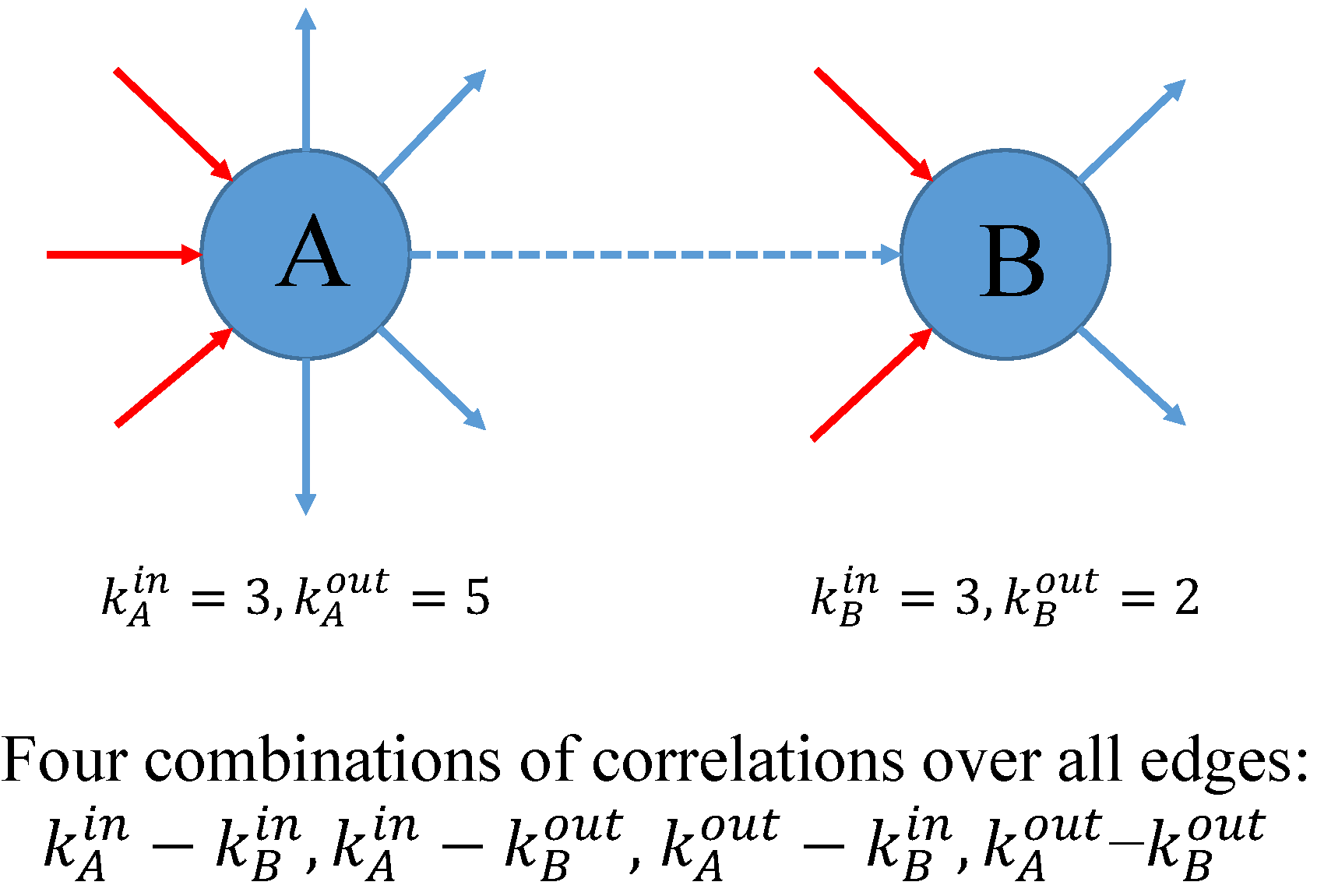
Matters become even more complex for the higher-order structural correlations. Taking the directions of edges into account (as in Figure 1), two types of nodes (giving and receiving) give rise to four types of relationships and four versions of ANND and ANNS for each node i: in-in, in-out, out-in, and out-out versions of ANND and ANNS, e.g.,
and
with the other three types of statistics being obtained by replacing in-degrees and in-strengths by the pertinent entities.
In each version, the interpretation of the relationship between the ANND and node degree and between the ANNS and node strength is similar to the one for the measures discussed in the undirected case. That is, a negative (positive) relationship signals disassortativity (assortativity) in the respective class of relationships.
Similarly, the four possible combinations between giving and receiving nodes are associated with four global assortativity coefficients, i.e., , , , and (see, for example, [32,33,34]). Note that in the Appendix A we provide additional details concerning these measures. Their weighted counterparts are , , , and . The algorithm for calculating these binary (weighted) coefficients is still similar to the one used for (or for the weighted case), except for the requirement that the directions of edges (see Figure 1) must be taken into account.
Clustering Coefficients
Clustering coefficients also come in four different versions in the directed network. The different types are exhibited in Figure 2. The local binary clustering coefficient in a directed network associated with cyclical clustering is, for example, defined as:
Note that, in the binary case we have , so that
and other types are obtained by appropriate variation of the indices, where is the number of nodes j in the neighborhood of the node i such that .
The local clustering coefficient associated with cyclical combination in the directed weighted version is defined as
2.3. Configuration Models
In this section we will summarize the main ideas behind the algorithm involved in the extraction of hidden (latent) variables from an observed network and their role in the network randomization process (see, for example, [12,13,15,16,17]). For a more detailed explanation of the derivation of the family of Exponential Random Graph Model based on the maximum-entropy method, as well as on how to use the maximum-likelihood method to solve for the hidden variables under given constraints, we refer readers to the studies by [12,35,36].
Undirected Binary Configuration Model (UBCM)
In the UBCM, briefly, the entropy of a randomized ensemble of networks is maximized under the constraint that the node degrees in the observed network should match the averages of node degrees in the randomized ensemble. Mathematically, we need to solve the following system of n equations to obtain the non-negative hidden variables that carry the information from the constraints and allow us to perform an efficient unbiased sampling of the ensemble
Once obtained, the hidden variables can be used to compute the probability of a link between any two nodes i and j, which in turn allows us to easily sample the ensemble associated with the above constraints
where is the notation for the expectation of over the ensemble.
Directed Binary Configuration Model (DBCM)
In the DBCM, the constraints are the observed out-degree and in-degree sequences and . We need to solve the following system of 2n equations to obtain the associated non-negative hidden variables and
The probability of a link from node i to j is given by
and the probability of a link from node j to i is given by
Undirected Weighted Configuration Model (UWCM)
Similarly, suppose that in an undirected weighted network we want to extract n hidden variables associated with the observed strength sequence , (). The maximum likelihood method involves solving the following system of n equations for the hidden variables
The expected link weight between node i and node j is given by
The probability of a link weight between node i and node j in the UWCM is
for , where is the probability of a link between two nodes , which is given by
Directed Weighted Configuration Model (DWCM)
In the DWCM, the constraints are the observed out-strength and in-strength sequences (i.e., and ). Mathematically, we need to solve the following system of 2n equations to obtain the hidden variables and , which are respectively associated with and
The expected link weights between node i and node j are given by
and the probability of a link weight from node i to node j in the DWCM is the same as in the Equation (21).
Undirected Enhanced Configuration Model (UECM)
In the UECM, we use both the degree sequence as well as the strength sequence as constraints. The associated non-negative hidden variables and () are then the solution to the following system of 2n equations
It should be noted that, in the UECM, the probability of a link (i.e., ) and the expected weight (i.e., ) between node i and node j depend on the information encoded in the strengths as well as in the degrees. More specifically, they are given by
and
In this model the probability of a link weight between two nodes is given by
where , and is defined by Equation (26).
Directed Enhanced Configuration Model (DECM)
In the DECM, the non-negative hidden variables , , , (, ) extracted from the four sequences of constraints , , , and are the solution to the following system of 4n equations
Similar to the UECM, in the DECM, the probability of a link (i.e., ) and the expected weight (i.e., ) from node i to node j depend on information encoded in the two sequences of observed degrees as well as in the two sequences of observed strengths. More specifically, we have
As it is obvious from the above derivations, the hidden variables are estimates of the inherent propensities of nodes to form links, and of the strength (volume) of those links. They could, in principle, be related to exogenous attributes of the nodes (like their size or balance sheet attributes). However, since we only have identification codes, not the real identities of banks available, no such analysis could be provided here. However, what we could do is to inspect the predicted link probabilities and weights on the base of the estimated hidden variables. We provide such an analysis at the end of Section 5.3 supported by graphical representations of these variables in Appendix B. Once we have estimated the hidden variables, the expected values of the second and third structural correlations in the randomized networks can be analytically computed or numerically approximated by taking the average over a simulated ensemble. In our study, for each considered null model, we generate an ensemble of 1000 randomized networks, and then take the averages of the measures in question over the ensemble.
3. Data and Summary Statistics for the Italian Interbank Market e-MID
The Italian electronic market for interbank deposits (e-MID) is organized on an electronic platform. The trading that takes place in this market is very transparent in the sense that the quoting bank’s ID, the market side label (i.e., “buy” or “sell”), the maturity, the interest rate, and the volume are visible to all other banks (for a more detailed description of the e-MID dataset, we refer readers to the studies of [20,21], or to the e-MID website http://www.e-mid.it/). It should be emphasized that this is the only electronic market for interbank deposits in the Euro Area and the US, and it plays a crucial role in liquidity pooling. According to the European Central Bank (see [37]), in 2006 e-MID accounted for 17% of total turnover in the unsecured money market in the Euro Area.
In our study, we use quarterly data for the e-MID market over the period from 1999 to 2010. The transactions between banks are aggregated into quarterly data, since at the higher frequencies (e.g., daily transactions) the matrix of the trades between banks is very sparse. From a network perspective, we are more interested in existing long-term relationships (credit lines) rather than in single transactions. Since such credit lines will typically not be serviced each day, a sufficiently long horizon is necessary to extract such information from the data (see [21] for a discussion of different aggregation levels of the data). In addition, we restrict our analysis to the Italian banks participating in this market, because foreign banks have not been very active in this market. Particularly, from the onset of the financial crisis in 2008 onward, non-Italian banks have basically withdrawn from this electronic market (e.g., see [20]).
In what follows, we briefly discuss some of the basic properties and statistics of the e-MID market data. In general, we observe that the number of active banks substantially declines over time, from 205 banks in the first quarter of 1999 (Q1) to only 90 banks in the last quarter of 2010 (Q48) (see Figure 3). As argued by [21], this decline was mainly driven by mergers and acquisitions among Italian banks during the sample period. Unfortunately, due to limited information, we can not implement a further analysis of these activities in the Italian banking system. In contrast, up to the financial crisis, we observe an increase of the average weights and density in the network (see also Figure 4a). These results signal an increase of market concentration since the system becomes smaller but the interactions among banks intensify.
We now summarize the fundamental statistical properties of the e-MID network over the period 1999 to 2010. A deeper analysis of these properties can be found in other studies such as [21,22,23].
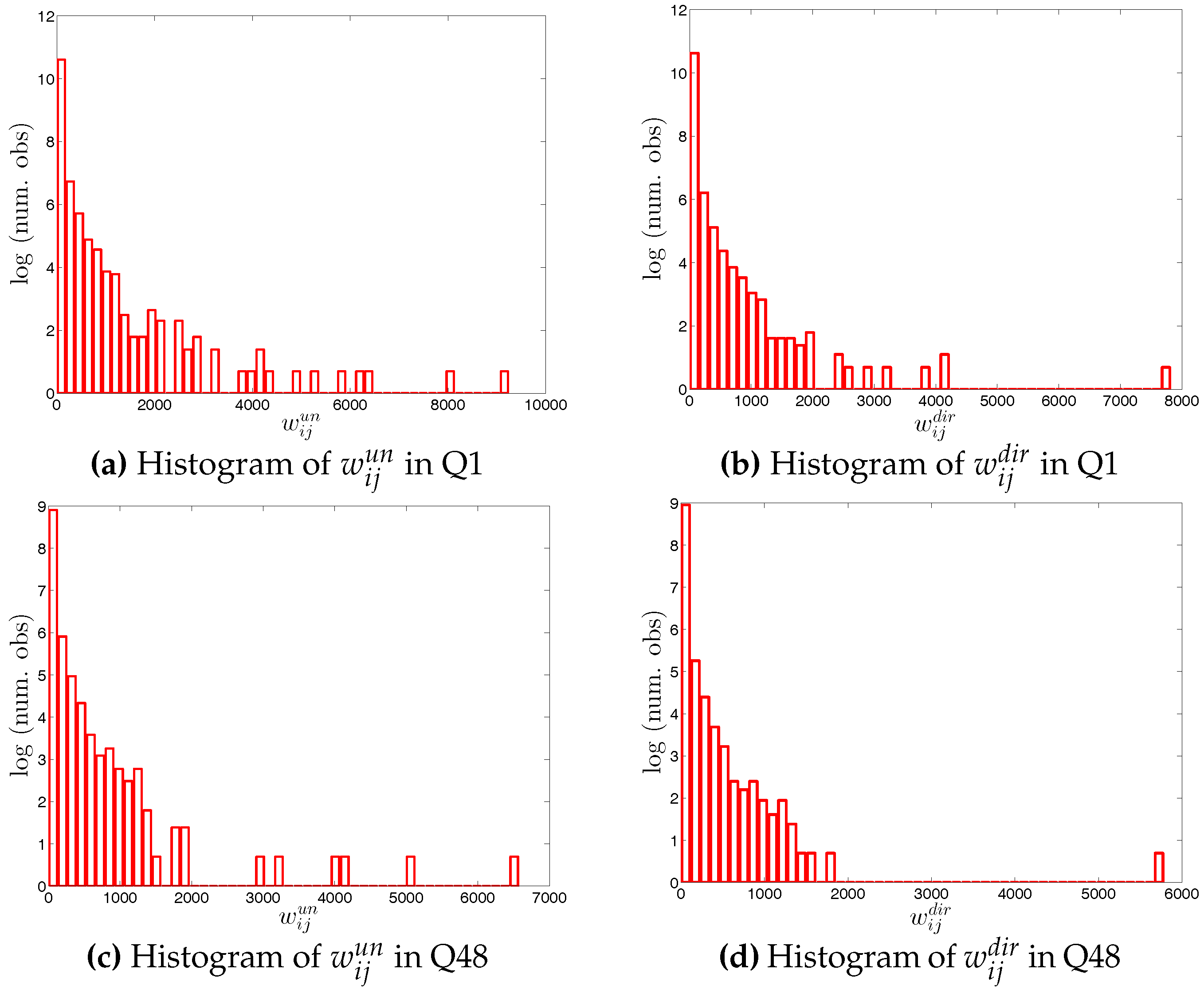
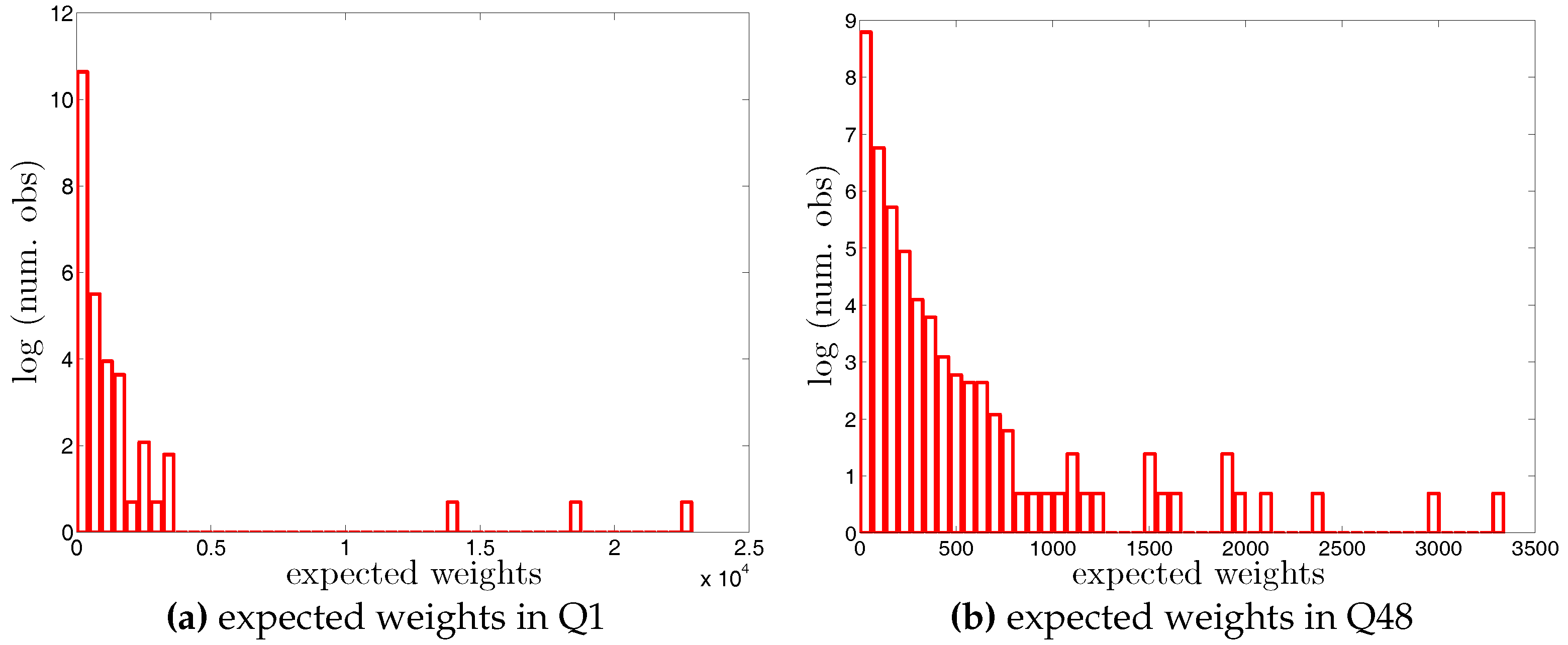
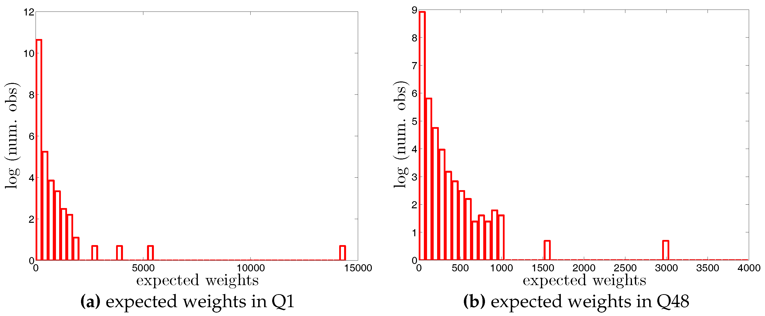
Looking at the distributions of the weights in the network (see Figure 4 and Figure 5), our first impression is that the trading volumes among banks are highly heterogeneous in the presence of some very large outliers. Another interesting observation is that the median of weights is always equal to zero. These findings imply that the network is generally sparse and the total trading volume is mainly driven by a small number of transactions. This may be a consequence of a hierarchical network structure. As [23] show, the e-MID market exhibits a core-periphery structure in which there is a group of banks in the core acting as intermediaries for the whole network and contributing to the majority of transactions.
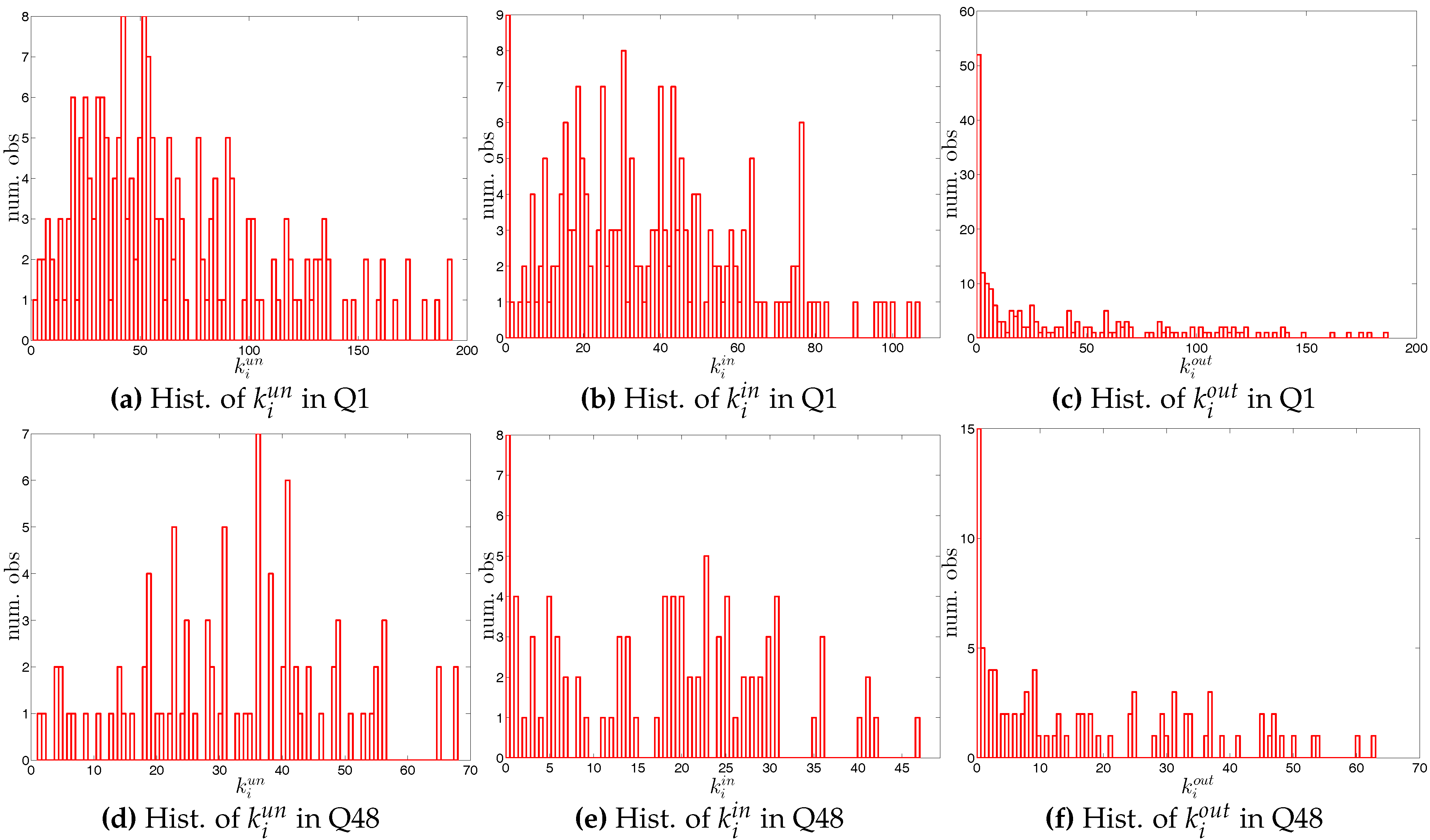
The statistics of bank degrees are summarized in Figure 6 and Figure 7. Most of these statistics generally decline over time as a consequence of the decreasing size of the network. In addition, we find that the distributions for different types of degrees can be very dissimilar. In particular, on the one hand, while the mean values of and are identical (by definition), the median of is much higher than that of . On the other hand, the range of (from zero to the maximum of ) is wider than the range of (from zero to the maximum of ). The markedly positive level of skewness observed in the distribution of , which is shown in panel (d) of Figure 6, indicates that the right tail is longer.
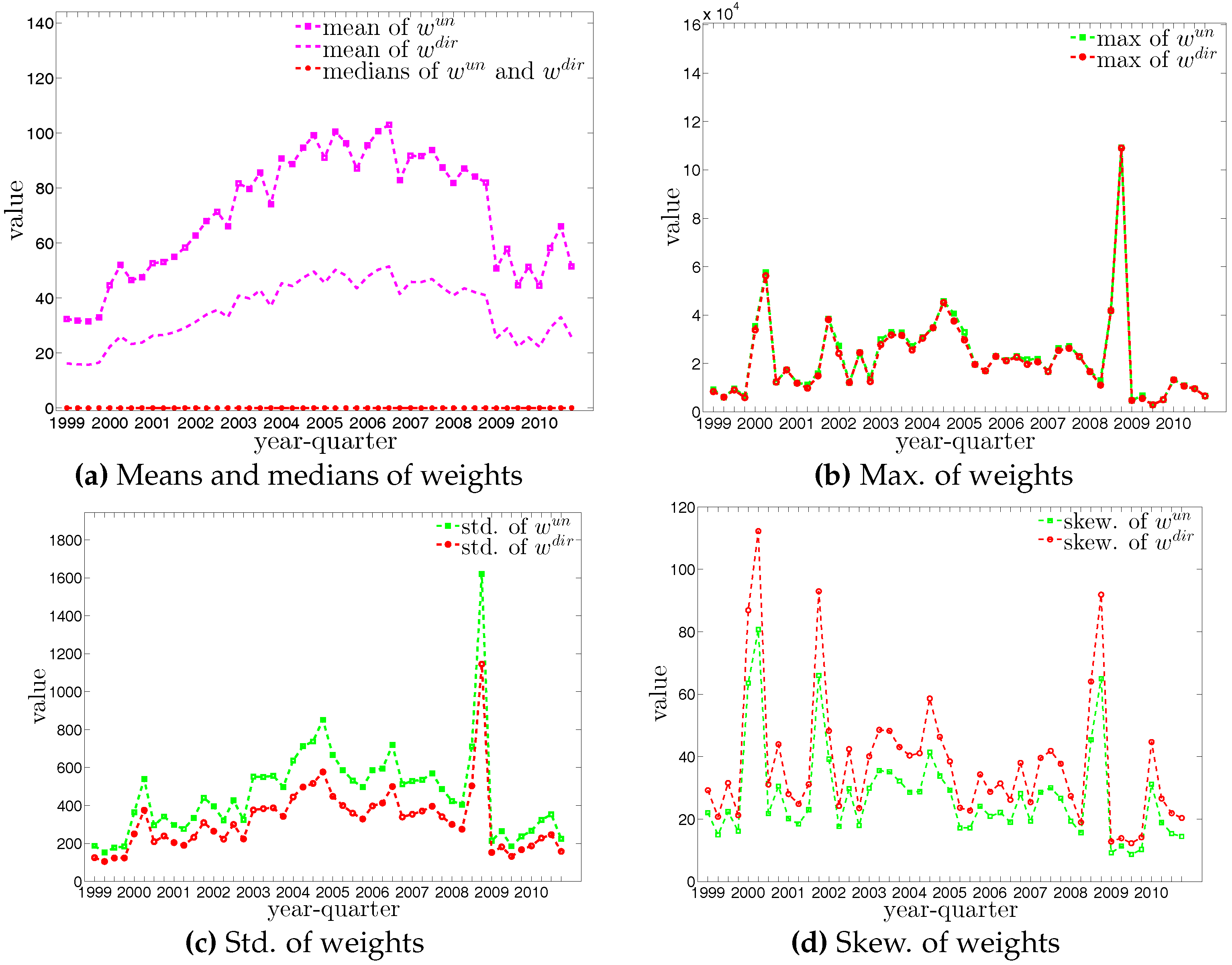
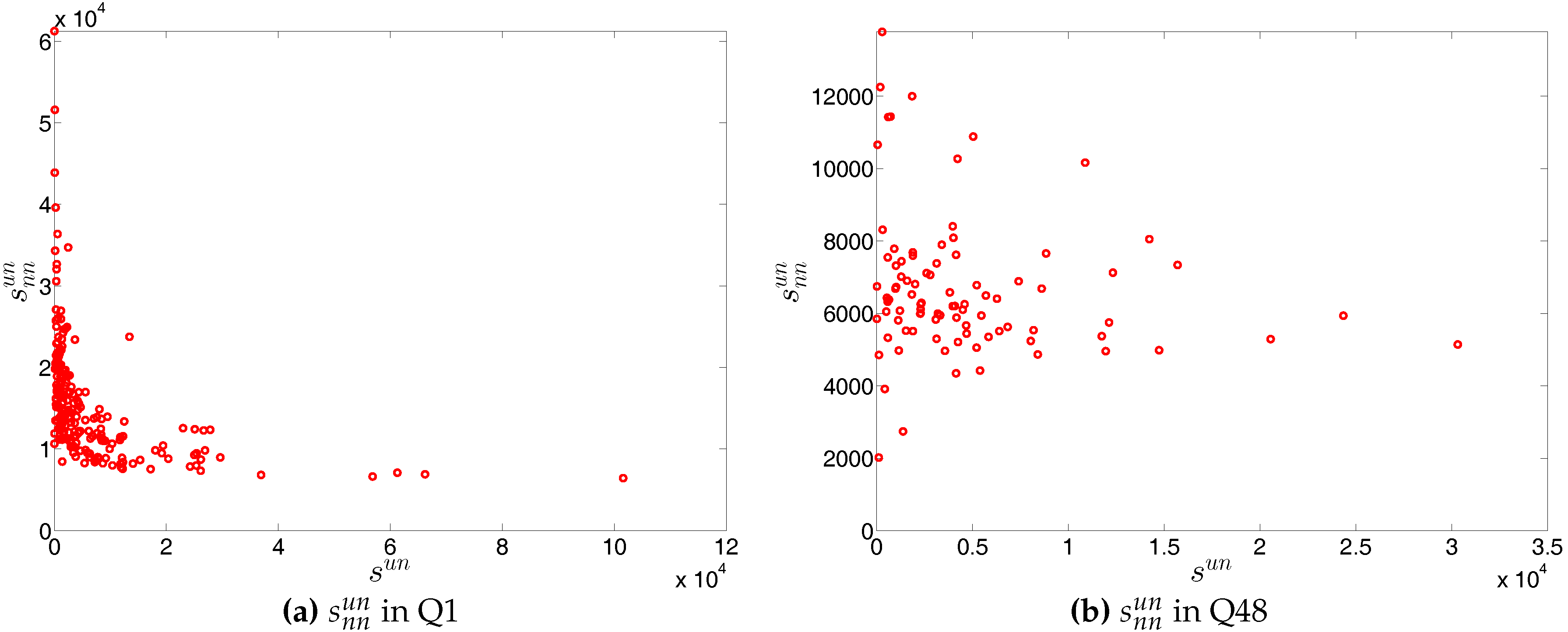
The four panels of Figure 8 show the evolution of the statistics of bank strengths over time. For all types of strengths, the mean value is always larger than the median. Furthermore, the distribution of each type of strength ranges from zero to an enormous value, with the mass of the distribution concentrated on the left. In addition, we also observe that the strengths of some banks are much larger than those of the rest (see Figure 9). In the presence of particular banks acting as global hubs, which trade with most other banks, it is intuitive that the strengths of these banks far exceed the mean value and the median.
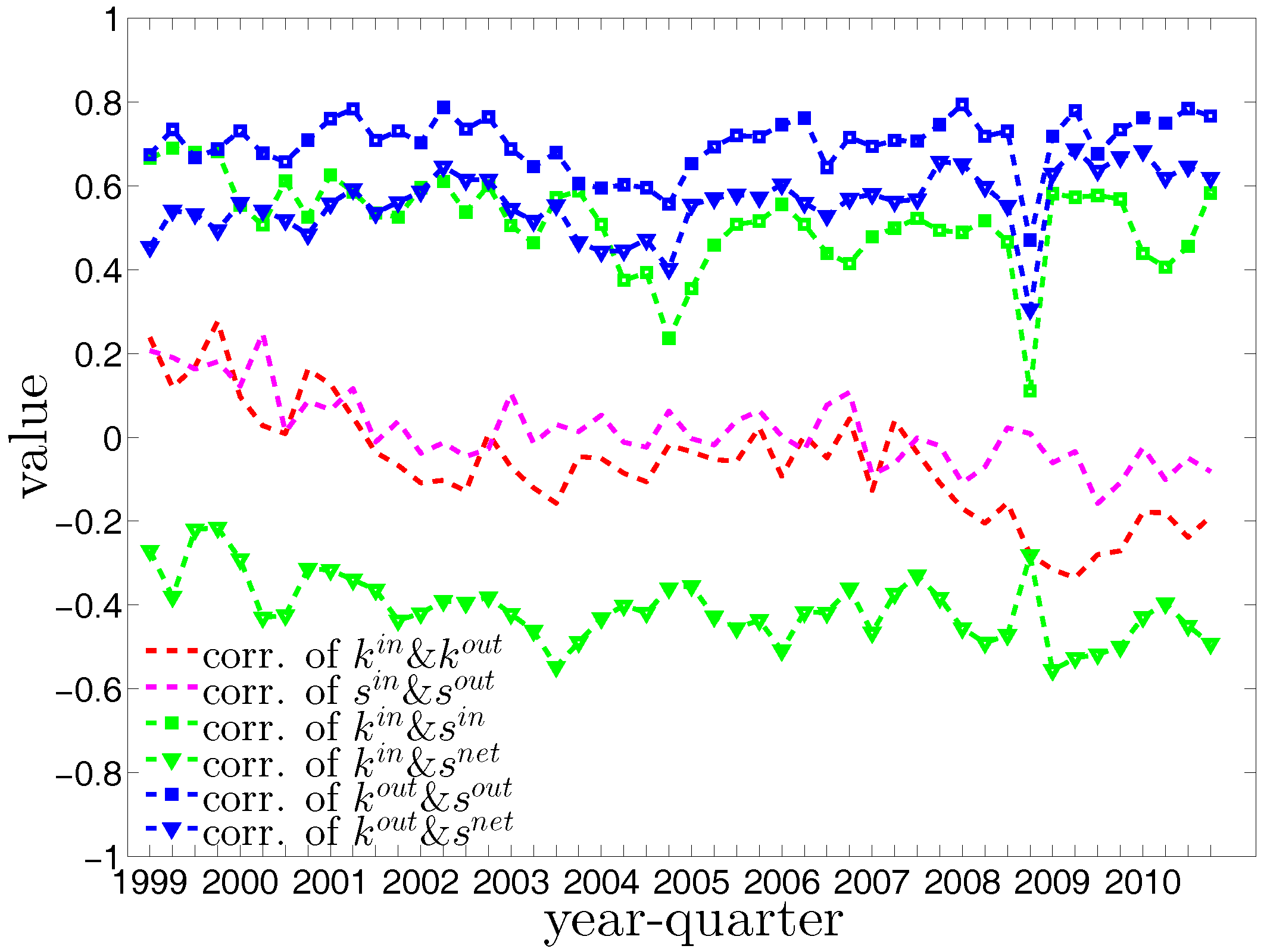
A closer inspection of the correlations between degrees and strengths in Figure 10 reveals an interesting behavior, i.e., banks become specialized in either predominantly lending or borrowing activities. Overall, the correlations between and and between and decrease over time. The correlations of other combinations of degrees and strengths show that, in general, banks with higher out-degrees tend to have higher out-strengths as well as higher net-strengths, while banks with higher in-degrees tend to have higher in-strengths as well as lower net-strengths (the net-strength, , is defined as ). As any bank can be a borrower or a lender within a period, its net-strength can be either negative or positive. In our analysis, we typically observe that banks with the highest out-degrees have a positive net-strength. In contrast, the banks with the highest in-degrees have a negative net-strength.
4. Findings for the Binary Network
4.1. Structural Correlations in the Undirected Binary e-MID Network
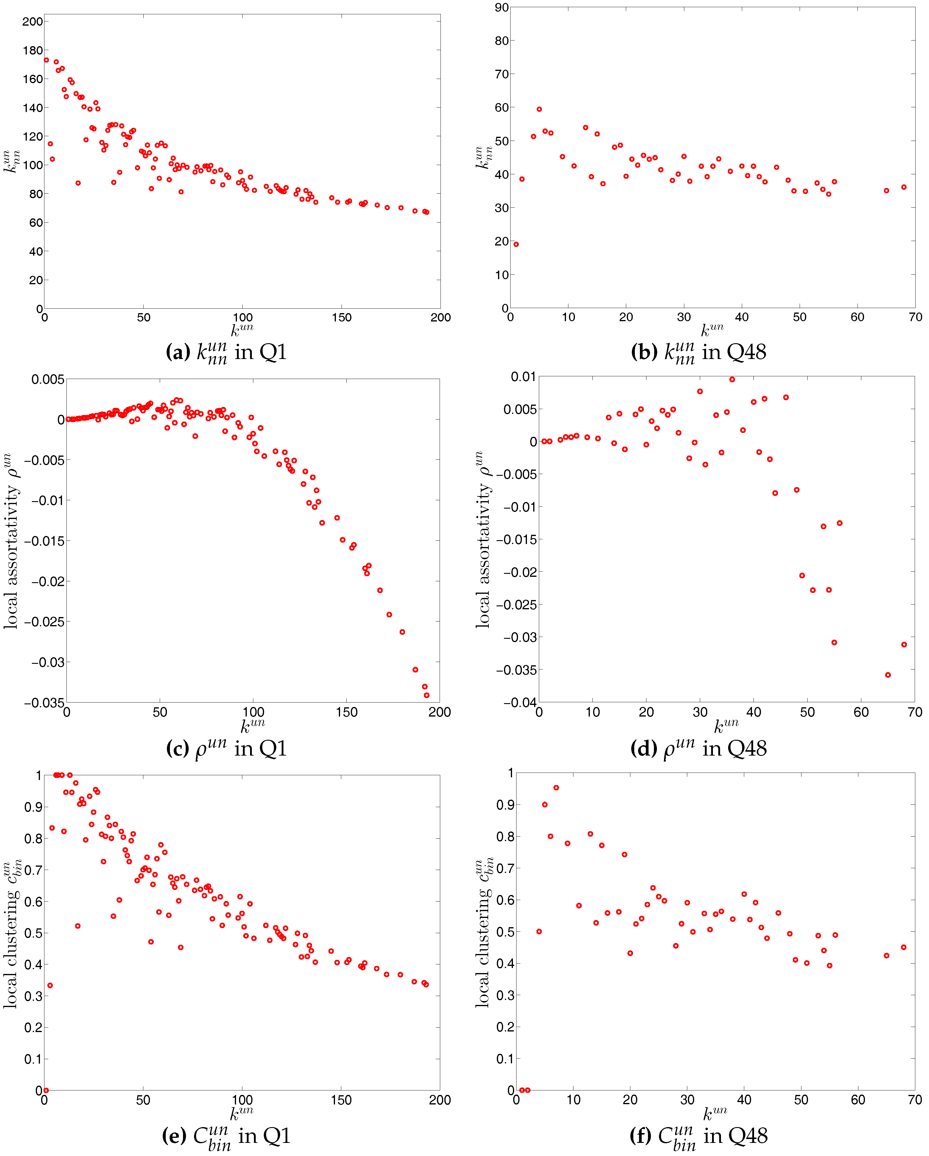
We first investigate the degree dependencies in the undirected binary e-MID network by examining the relationship between the node degree () and the average degree of its neighbors (). The overall disassortativity in this version of the network is evidenced by the negative relationship between these two quantities as shown in Figure 11a,b, in which the measures for the networks from Q1 (the first quarter in our data set) and from Q48 (the last quarter in our data set) are plotted as an example. Note that the overall negative correlation between and is also observed in all 48 quarters from 1999 to 2010. In addition, generally, we find that the absolute value of this correlation is declining over time.
Next, we now turn to the Pearson correlation coefficient of degrees as an overall indicator of degree dependencies in the network. As shown in Figure 12, over time, overall, the network exhibits disassortativity as signaled by the negative coefficient. Consistent with what we discovered in our analysis of the measure ANND, the absolute value of is also declining from 1999 to 2010. The presence of pronounced disassortativity in the undirected binary version of the network implies that, overall, high (low) degree banks tend to have transactions with low (high) degree banks. This supports the finding of [23] of a core-periphery structure in which a subset of money center banks with many links are the main actors in the interbank market, and the less active peripheral banks mostly trade with a small number of these core banks to invest their liquidity overhang or to obtain funds in the presence of a liquidity deficit. It is not obvious whether the decrease of the absolute value of signals a tendency towards a weaker core-periphery structure or whether it is merely a consequence of the decrease of the number of banks over our period of observation.
For a more comprehensive assessment of the degree dependencies in the network, we employ the local assortativity coefficients that indicate the contribution of each node to the global level of assortativity (see the Appendix A for further details). The basic idea is that the numerator in the Pearson correlation coefficient proposed by [25,26] can be reformulated based on the contribution of the individual nodes instead of in terms of the edges (see, for example, [38]) leading to the decomposition
In Figure 11c,d we plot against to investigate which nodes (in terms of their degrees) contribute most to . It appears that the hubs are the main contributors to the overall disassortativity of the network, while smaller degree nodes sometimes exhibit positive assortativity. This also reveals that adding or removing a hub from a network may have a large impact on its overall mixing nature, and this decomposition underlines the segmentation of the banking sector into a core and a periphery in terms of banks’ activity in the money market.
For the third order correlations, we employ the local clustering coefficient proposed by [39]. In this simple version of the network (undirected binary case) clustering refers to the extent to which two connected nodes in the network have common neighbors. We observe that, overall, the undirected local clustering is a decreasing function of degree (Figure 11e,f), meaning that the neighbors of highly (poorly) connected banks are poorly (highly) interconnected. In fact, this relationship is typically found in many real world networks exhibiting a high heterogeneity in the degrees and a disassortative mixing nature (e.g., see [40]). In our network, the bank degrees are highly heterogeneous, and the small (large) degree banks seem to have larger (smaller) local clustering coefficients because they are mostly connected to large (small) degree banks.
The evolution of the average of the undirected local binary clustering coefficients over all nodes, , is shown in Figure 13, where we can see a significant reduction in around the time of the financial crisis, revealing an overall decrease in clustering. Intuitively, during that period, banks may have cut down on their lending/borrowing linkages, which would affect the clustering coefficients from that period on average. This finding is in harmony with the results of [41], which estimates a behavioral model for link formation for the same data set and find a higher tendency to avoid indirect exposure as indicated by clustering effects for the period after 2007.
4.2. Structural Correlations in the Directed Binary e-MID Network
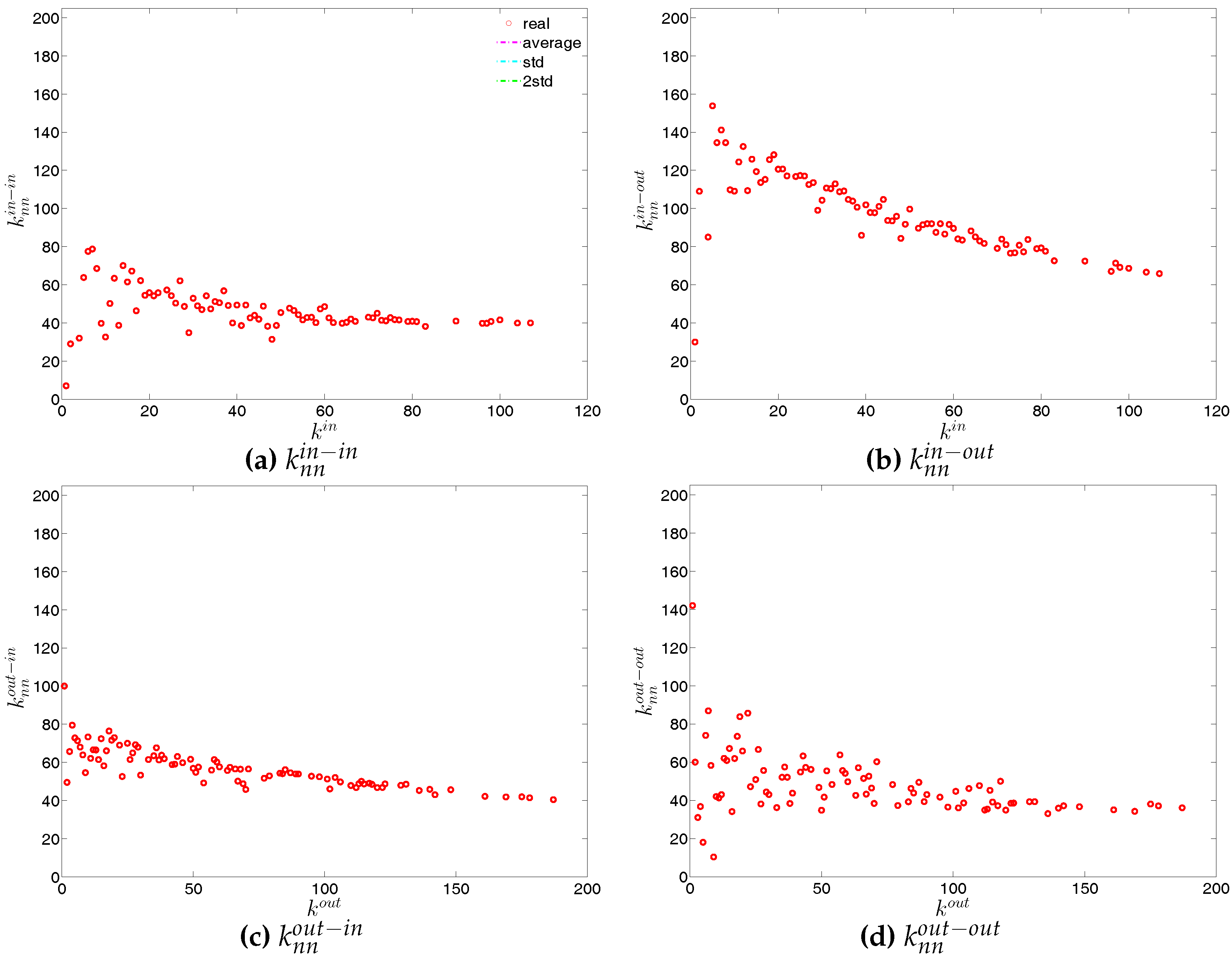
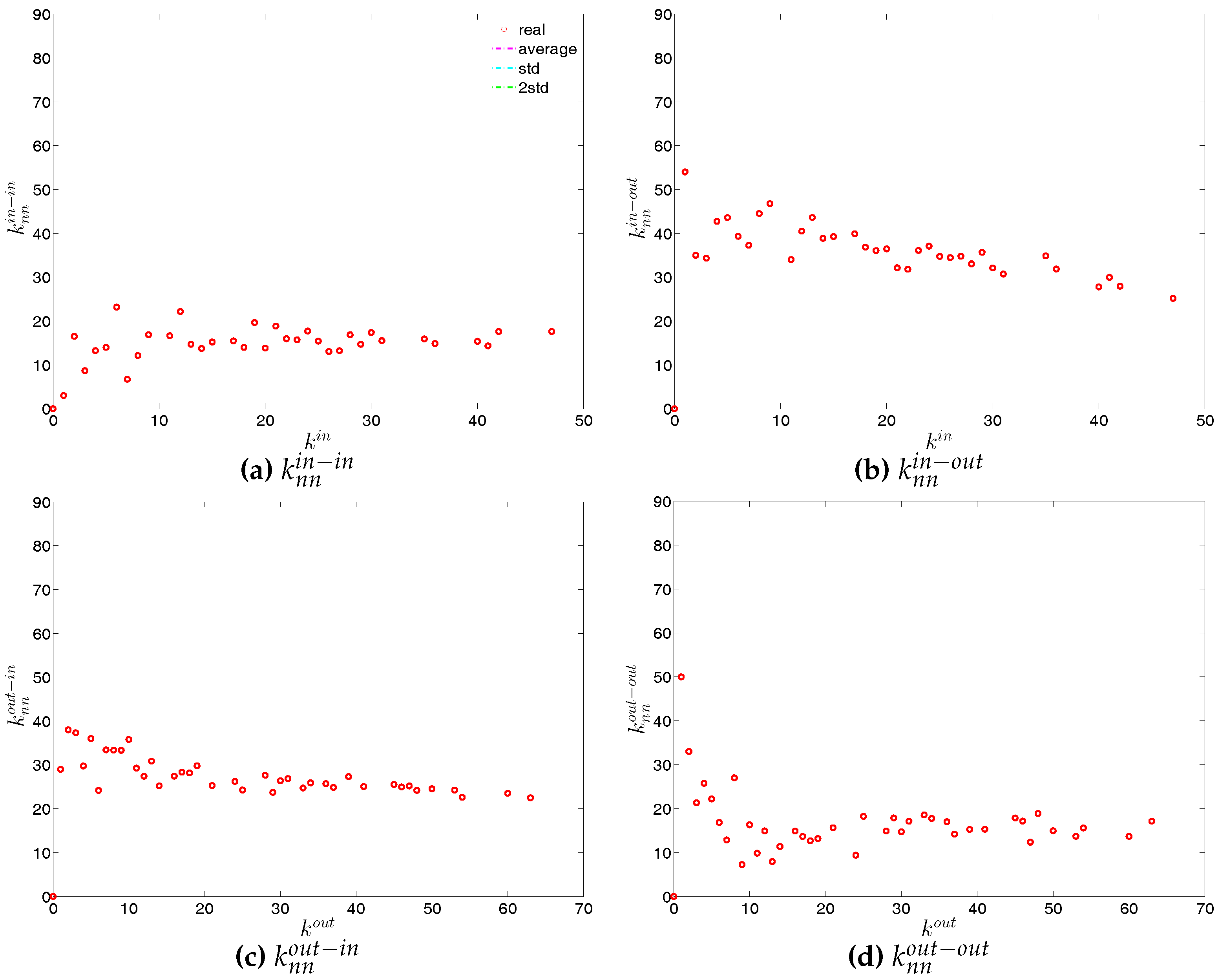
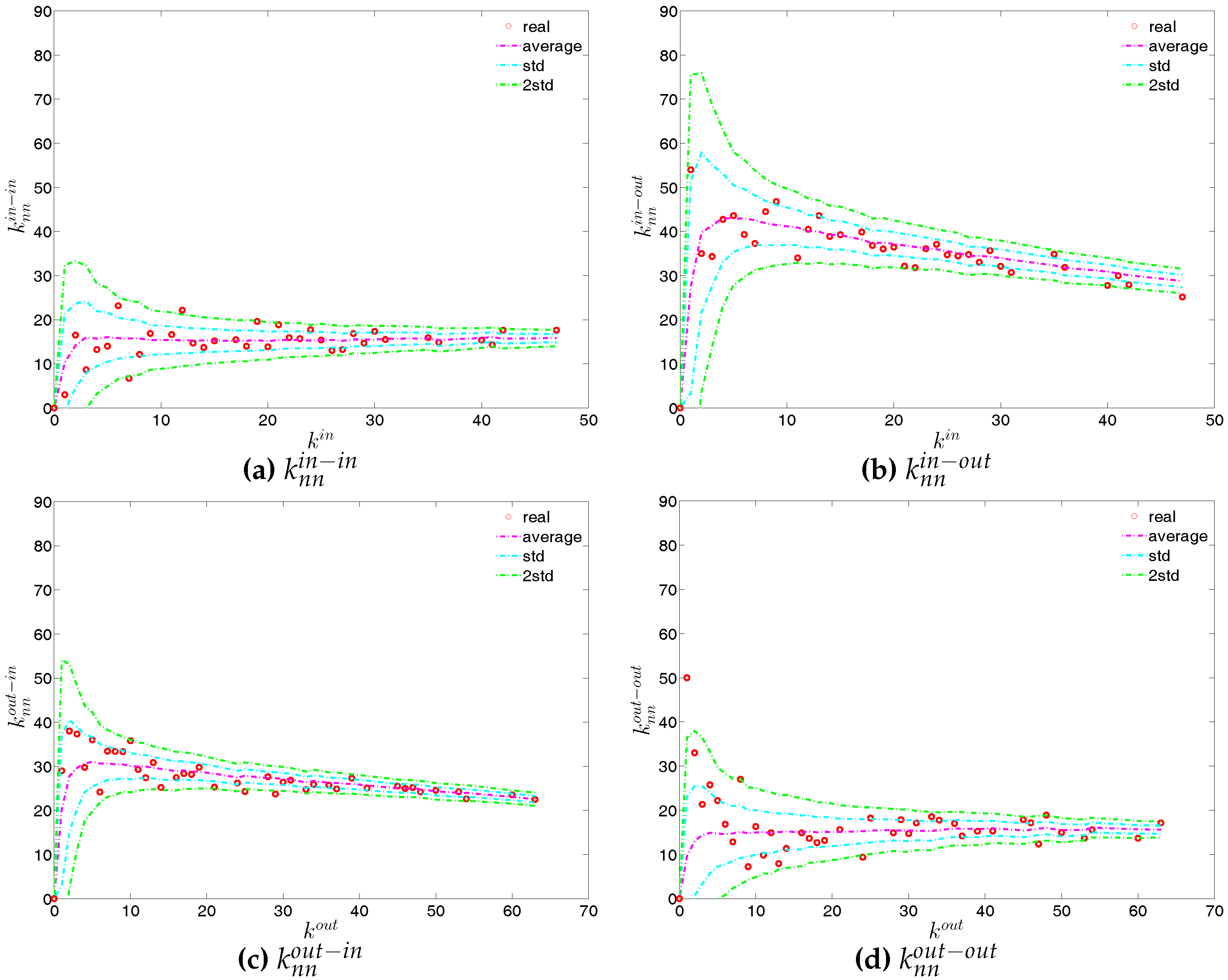
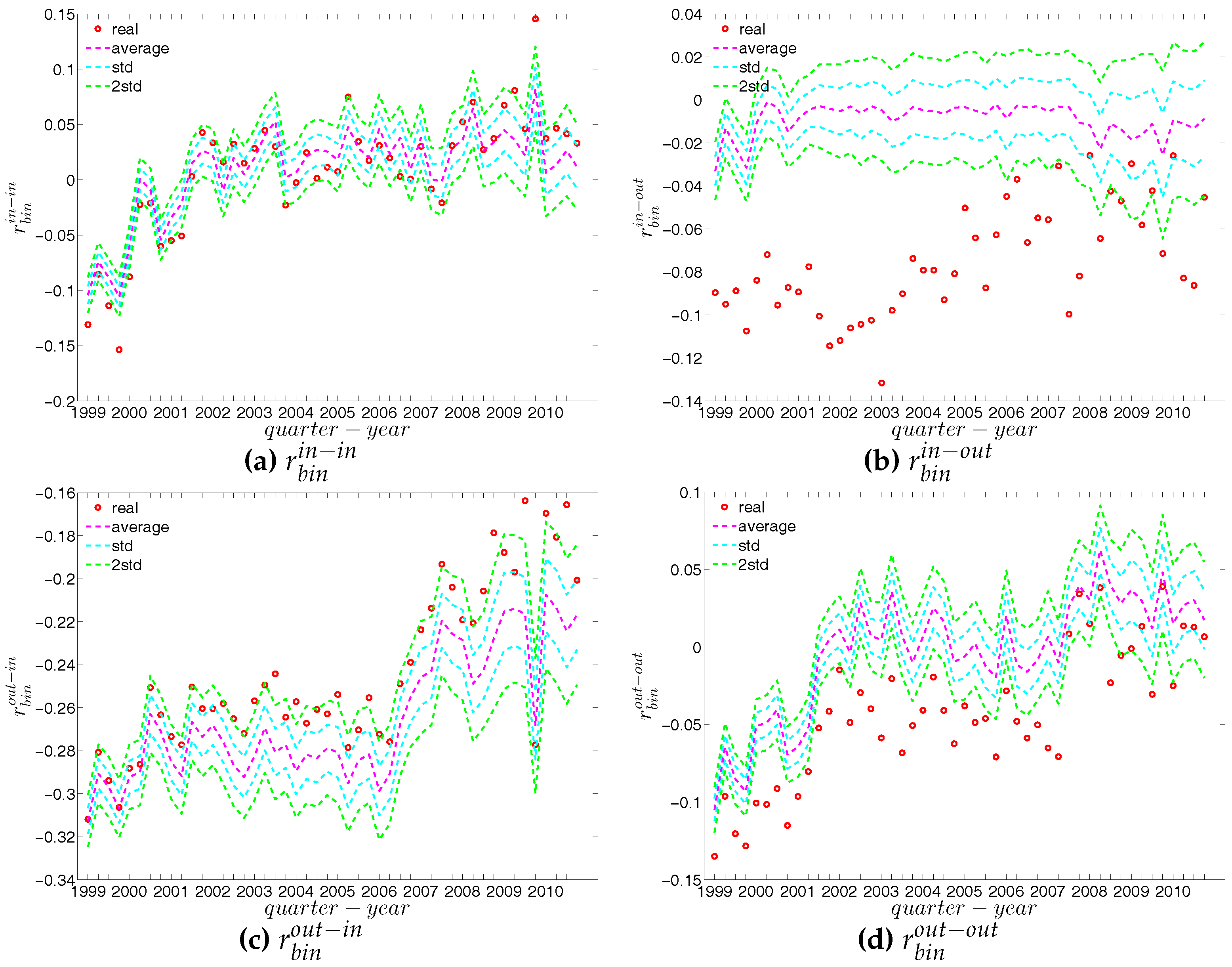
We now extend our analysis to the directed version of the binary network. Figure 14 and Figure 15 show the relationship between ANND and node degree for the four types of mixing, i.e., in-in, in-out, out-in, and out-out. In the same network some types of mixing can be assortative, while others disassortative. For instance, while in Q1, overall, ANND is a decreasing function of the associated degree in all four cases, this relationship breaks down for the in-in and out-out mixing in Q48. In contrast, the overall negative correlation between ANND and the associated degree for the in-out and out-in mixing is observed in almost all quarters.
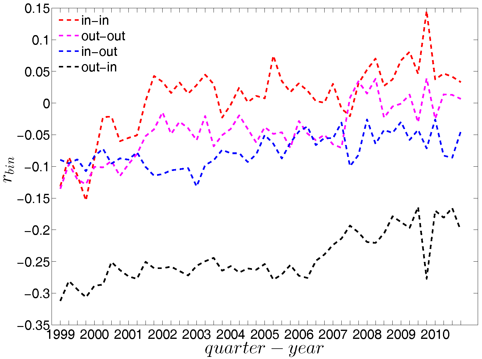
For a more general assessment of the overall mixing nature in the directed binary network, we calculate the Pearson correlation coefficient in each category of mixing and show its evolution over time (see Figure 16). In comparison to the undirected version, the directed binary network displays more complicated degree dependencies. We can see that and display a different behavior than and . More specifically, while in the out-in and in-out categories we persistently observe disassortativity in all quarters, the other two categories switch between displaying assortativity and disassortativity over time. The network under consideration seems to exhibit a very pronounced mixing nature only in the mixing category out-in. The interpretation of the mixing observed in the various categories is similar to the interpretation of mixing in an undirected binary network. For instance, a negative value of , signaling disassortativity in the out-in category, indicates that a high out-degree bank tends to have out-going links to low in-degree banks, and/or that a low out-degree bank tends to have out-going links to high in-degree banks. Again, this finding can be seen as an indicator of a periphery structure as suggested for the present data by [23]. The interpretation of the coefficients capturing the mixing in the other types of connections is analogous. In addition, the mixing we observe in the out-in category () comes closest to the one observed in the undirected network captured by and is overall consistent. The similarity between these two quantities was mathematically proven by [34]. Furthermore, although the in-out mixing category exhibits disassortativity, in many quarters the coefficient is very close to zero.
Similarly to the undirected case, we define the local assortativity measures for a given node i as , , , and corresponding to the four mixing categories in the directed version of the network (see the Appendix A for further details). Note that again equalities of the following form must hold:
and analogously for the other measures. The measures , , , and give us useful information about the contribution of each node to the respective overall assortativity indicators.
The local assortativity indicators in the two quarters Q1 and Q48 are respectively shown in Figure 17 and Figure 18. In these figures, each local assortativity indicator is shown as a function of the corresponding degree. Note that in the cases of and , we plot them against , since each of them depends on both and (see the Appendix A for more detailed derivations). The results indicate that, first, given an overall level of assortativity in a particular category, the contribution of nodes of different degrees varies across the four mixing categories. In the out-in mixing category, we observe that, on the one hand, the hubs contribute most to the overall level of assortativity; on the other hand, small degree nodes are characterized by small values of assortativity or disassortativity. In addition, the contributions of medium degree nodes are more volatile than those of the small degree nodes. This is very similar to what we found in the undirected version of the network. However, the behavior of the local assortativity indicators becomes more complicated for the other mixing categories. For example, the contributions of hubs and medium degree nodes can fluctuate a lot, so that it becomes difficult to classify which type of nodes plays an important role for the overall level of assortativity.
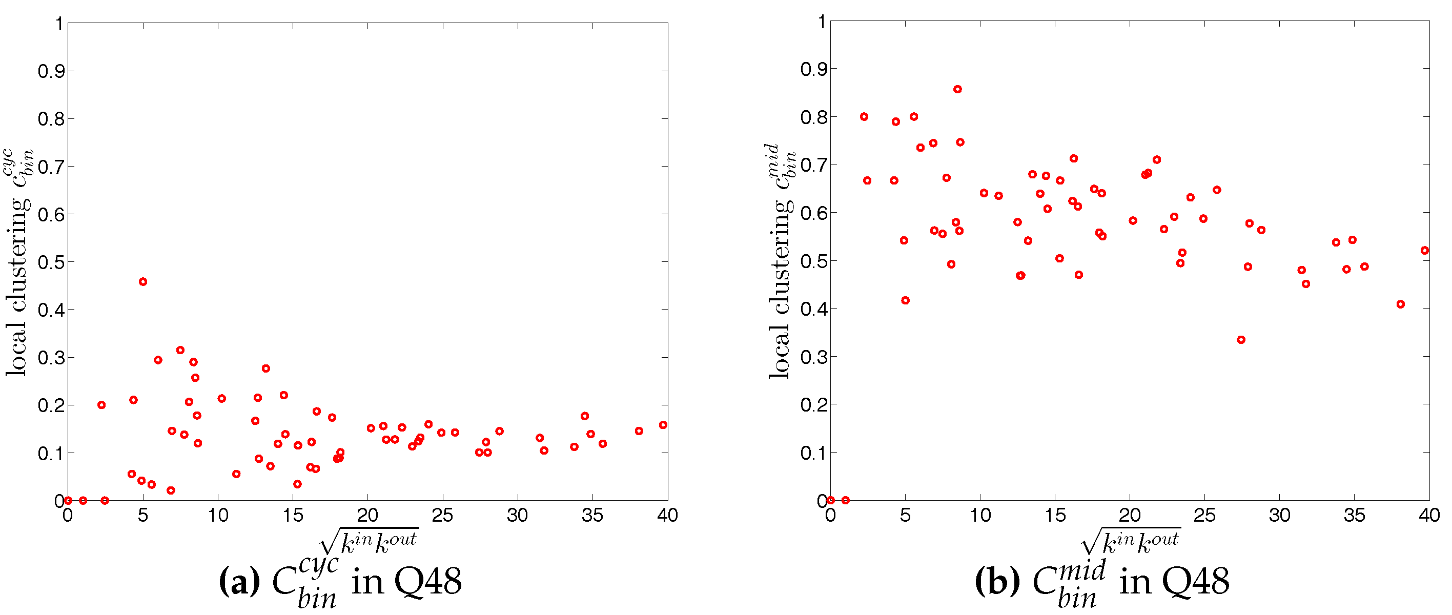
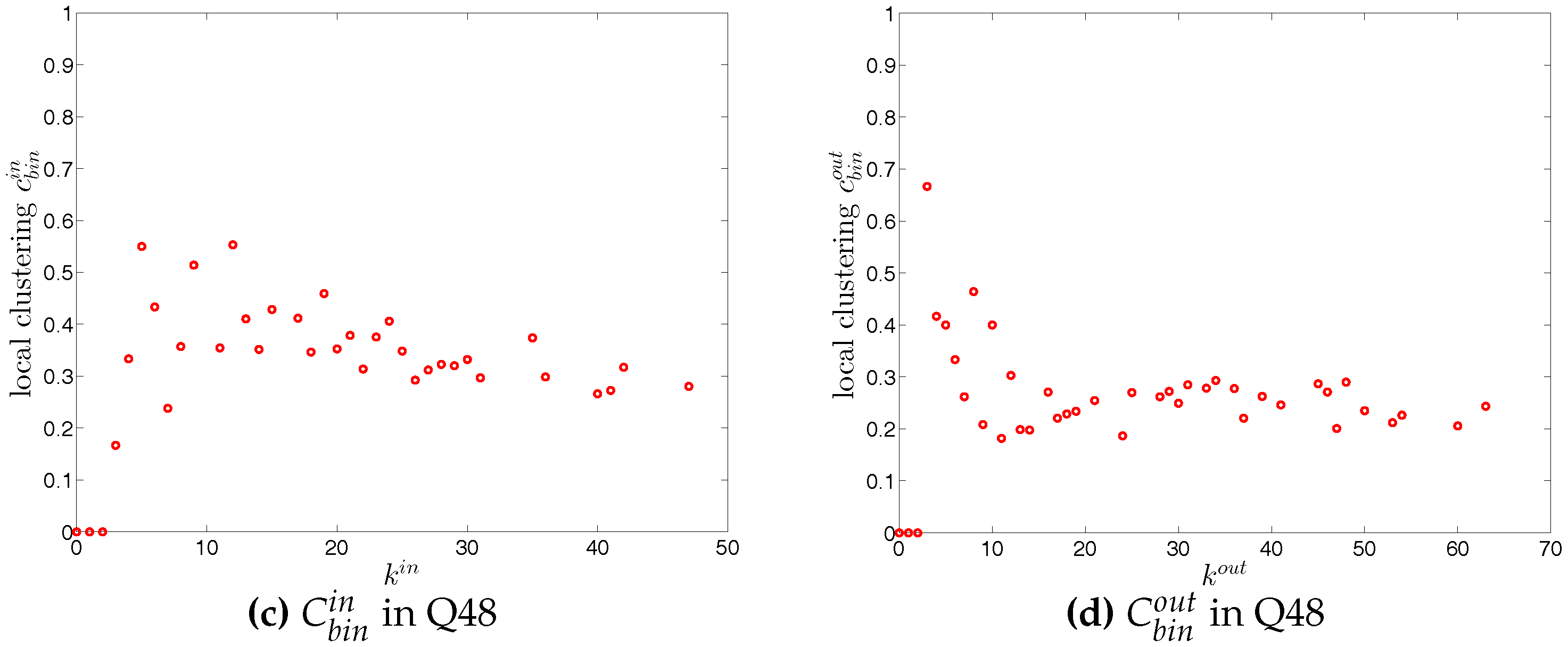
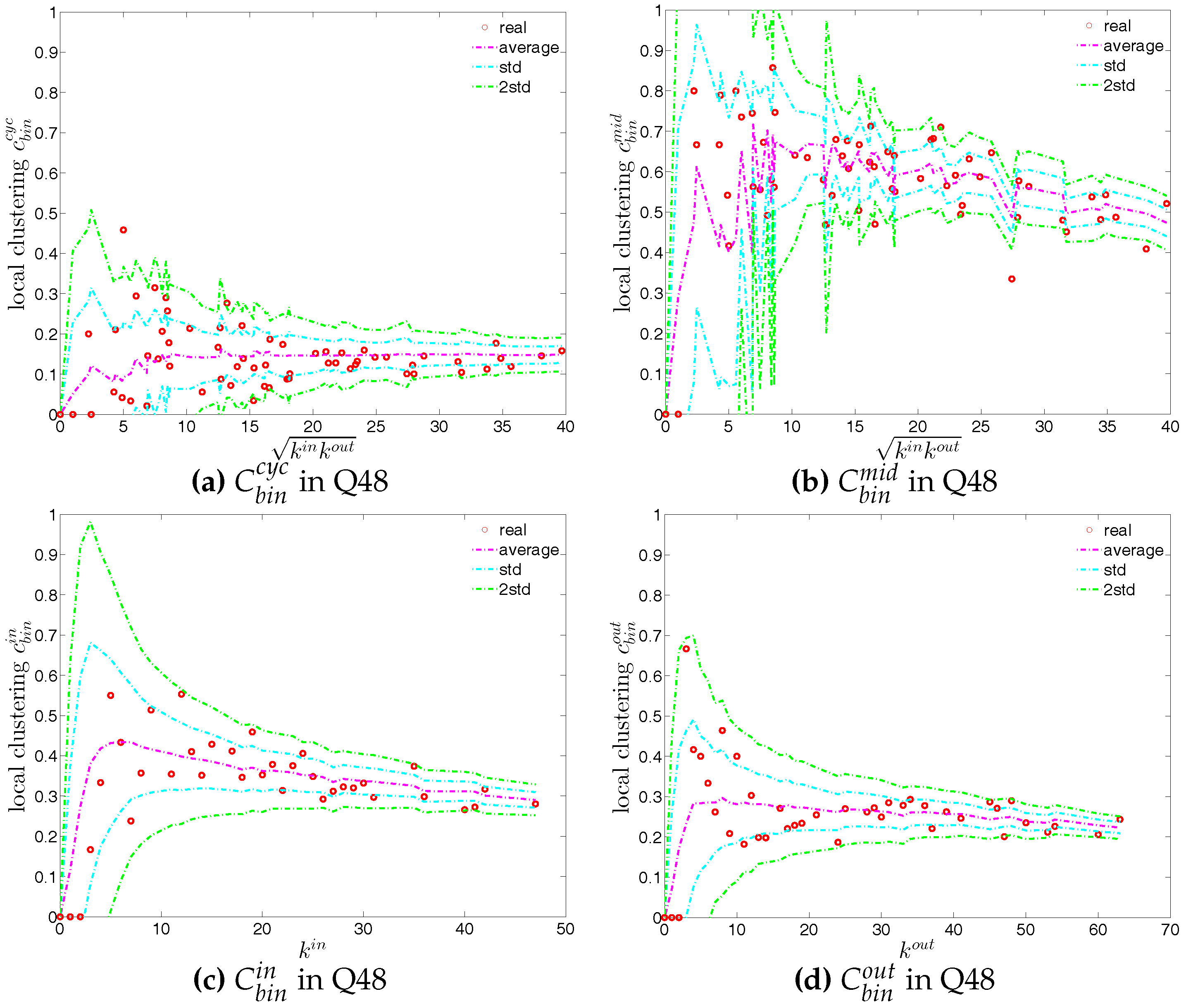
Next, we turn to the third order correlations between banks in the directed binary network. We focus on investigating local clustering as a function of degree for the four cases shown in Figure 2 (see, for example, [42]). In the following discussion we will be referring to nodes i, j, k as an example of three vertices in a network building a triangle. It is clear that the directions of the edges now matter for the clustering analysis. The measures , , and summarize the prevalence of a particular type of relationship that a node has with its neighbors. For instance, larger values of (see Figure 2b) may represent a higher systemic risk associated with that node, since bank i can be a source of risk as well as be exposed to risk from other banks. Clustering relationships of the type shown in Figure 2c are also conducive to systemic risk since a default of bank i would affect both its partners. Larger values of indicate a higher systemic risk dependence on the same funding sources in the interbank market. This is, however, not the case for cyclical clustering relationships (captured by ) since in this type of relationships exposures can cancel each other out (see Figure 2a). Finally, large values of associated with bank i indicate risk exposure of bank i itself, since both banks j and k can affect bank i in case either of them would default (see Figure 2d).
For each type of clustering relationship, we first consider the local clustering coefficient as the function of the corresponding degree (in the cases of and , we plot them against ). Typically, in each case, a general negative relationship is observed in the first quarters, but for later quarters this relationship becomes flatter (see, for example, Figure 19 and Figure 20).
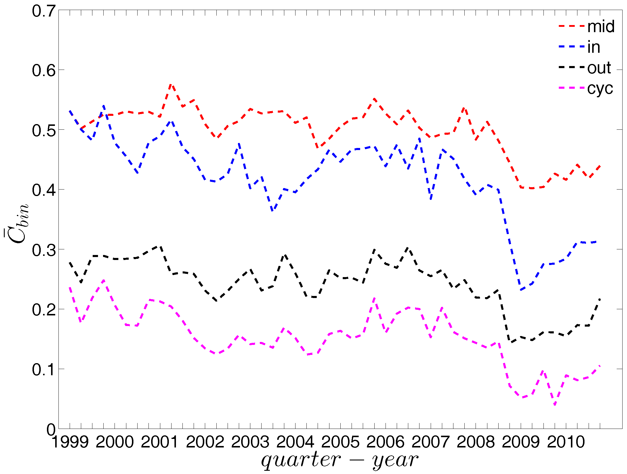
We now take the averages of the local clustering coefficients across all nodes (i.e., , , , and , respectively for the four different types) and then investigate their evolution over time. We observe that, first, for the most part, the averages , , , and are in descending order, with clustering relationships of the cyclical and out-type being much less common than the other two (see Figure 21). We consider this prevalence of the middleman and in-type clustering relationships as evidence of the presence of systemic risk in the network. Second, similarly to what we observed in the undirected network for , the averages of the local clustering coefficients for all four clustering types dramatically decrease around the time of the financial crisis, evidencing structural change in the third order correlations between banks.
4.3. Comparisons to the Configuration Models
When comparing the phenomenological properties of the data to those of the configuration models, we basically ask the question whether the higher-level characteristics are the mere consequence of the observed features of lower order. Features that could not be accounted for by the configuration model would indicate facets of the data that need additional behavioral explanations.
4.3.1. Undirected Binary Network
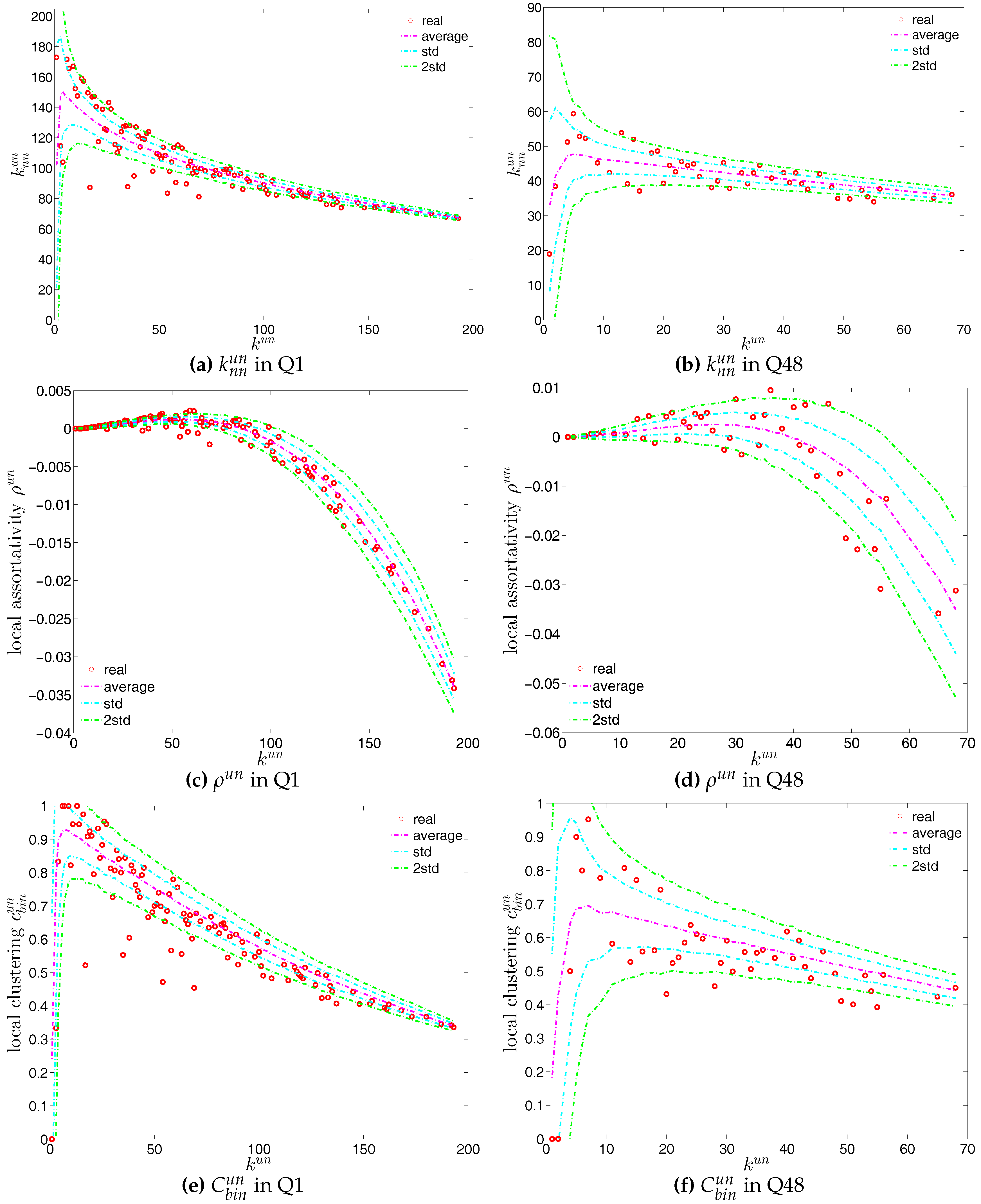
We first employ the undirected binary configuration model (UBCM), which maintains the intrinsic heterogeneity in the degree sequence of the undirected binary version of the observed e-MID network. Figure 22 shows a comparison between various higher order structural correlations observed in the e-MID network and the same structural correlations observed in the randomized ensemble for the first and last quarters. Note that, in each panel of Figure 22, besides the observed and the expected values (over the randomized ensemble), we also report the regions of standard deviation (std.) and ±2 std. away from the expectations. In most cases, as shown in Figure 22a–f, the local behavior of the structural correlations is well replicated by the UBCM. As shown in Figure 23a, the average of the ANNDs over all nodes (i.e., ) is also located inside the std. band when plotted over time. In contrast, in terms of our measure of global assortativity (), in almost all of the quarters, the observed values lie outside the std. band (see Figure 23b). A similar result is obtained for the evolution of the average of the local clustering coefficients () with many significant deviations, but the main trends of the observed and the expected values are similar (see Figure 23c).
4.3.2. Directed Binary Network
Recalling that under the directed binary configuration model (DBCM), both out-going and in-coming degrees are enforced on average over the ensemble, we show the comparisons between the structural correlations of observed network and those obtained from that model in Figure 24 and Figure 25 (for ANND), Figure 26 and Figure 27 (for the local assortativity indicators), and Figure 28 and Figure 29 (for the local clustering coefficients).
In addition, as for the undirected version, we also compare the evolution of the global indicators with the evolution of their expected values obtained from the DBCM. We show the results for the averages of the ANNDs (i.e., , , , ) in Figure 30, for the global assortativity indicators (, , , ) in Figure 31, and for the averages of the local clustering coefficients (, , , ) in Figure 32.
First, regarding the local indicators (see from Figure 24, Figure 25, Figure 26, Figure 27, Figure 28 and Figure 29), in most cases, the observed ANNDs, local assortativity indicators, and local clustering coefficients are in agreement with those evaluated under the DBCM. Since the few observed points significantly deviating from the expected ones do not reveal any patterns (under the DBCM), they might be seen as the expected rejections one obtains for a large sequence of simultaneous tests.
Second, regarding the evolution of the averages of the ANNDs, Figure 30 shows that, , , and always lie within the std. band, while is underestimated for most of the time.
Third, in terms of the global assortativity indicators, for the most part, and are located inside the ±2 std. band, while and are mostly being overestimated (see Figure 31). The difference between the null model and the data is particularly pronounced for . Note that while measures the correlation between the average number of loan connections of a creditor and the average number of loans taken up by a borrower, has the opposite orientation: it measures the correlation between the average number of loans (accepted from other banks) of the bank who is a creditor in a certain transaction with the average number of loans granted to other banks by the borrower in the same transaction. While the configuration model predicts a correlation close to zero in most periods for , the empirical statistics are significantly (more) negative. This indicates that disassortativity pertains in a more general sense between two typical partners of a credit transaction. They are not only unequal in the roles (lender, borrower) in which they appear in a specific transaction, but also if we look at the opposite roles: hence the association of large to small (core to periphery) in the majority of the trades is relatively independent of what aspect (lending or borrowing) we consider. The significant downward deviations of from the prediction of the configuration model also supports this view.
Finally, over time, the averages of the local clustering coefficients , , , and are generally in agreement with their expected values from the DBCM, as shown in Figure 32.
5. Findings for the Weighted Network
In the binary version of the observed network, we treat all edges as if they were homogeneous. However, in reality, the capacity and intensity of the relations between banks can be very heterogeneous, consequently the weighted version can have different properties compared to its binary counterpart. In this section, we investigate the structural correlations in the weighted e-MID network. For the sake of simplicity, we do not consider the local weighted assortativity in this section, since breaking down the overall weighted assortativity measure into the contributions of the individual nodes is much more complicated than in the binary case.
Regarding the null models, instead of preserving the observed degree sequence(s) as in the Binary Configure Models (i.e., UBCM, DBCM), first, we employ the weighted configuration model preserving the observed strength sequence(s) (i.e., the UWCM model in the undirected case and the DWCM model in the directed case) and examine whether the chosen null models can replicate the structural correlations in the observed weighted network. As a second step, we consider the enhanced configuration models which maintain both the observed degree as well as strength sequences (i.e., the UECM and the DECM respectively in the undirected and directed cases) and repeat the same exercise.
5.1. Structural Correlations in the Undirected Weighted e-MID Network
We report the strength dependencies in Figure 33 by considering the relationship between (ANNS) and in the first and last quarters. We observe that is generally a declining function of , although this feature becomes less pronounced towards the end of our time series. This relationship is confirmed by the negative value of the global weighted assortativity measure (see Figure 34). This signals that the prevalence of disassortative mixing in the undirected weighted e-MID network does not only apply to the degrees, but also to the strengths of nodes. Furthermore, it should be emphasized that, in comparison to the undirected binary version of the network, the undirected weighted network exhibits less disassortativity overall, since is smaller than in absolute value.
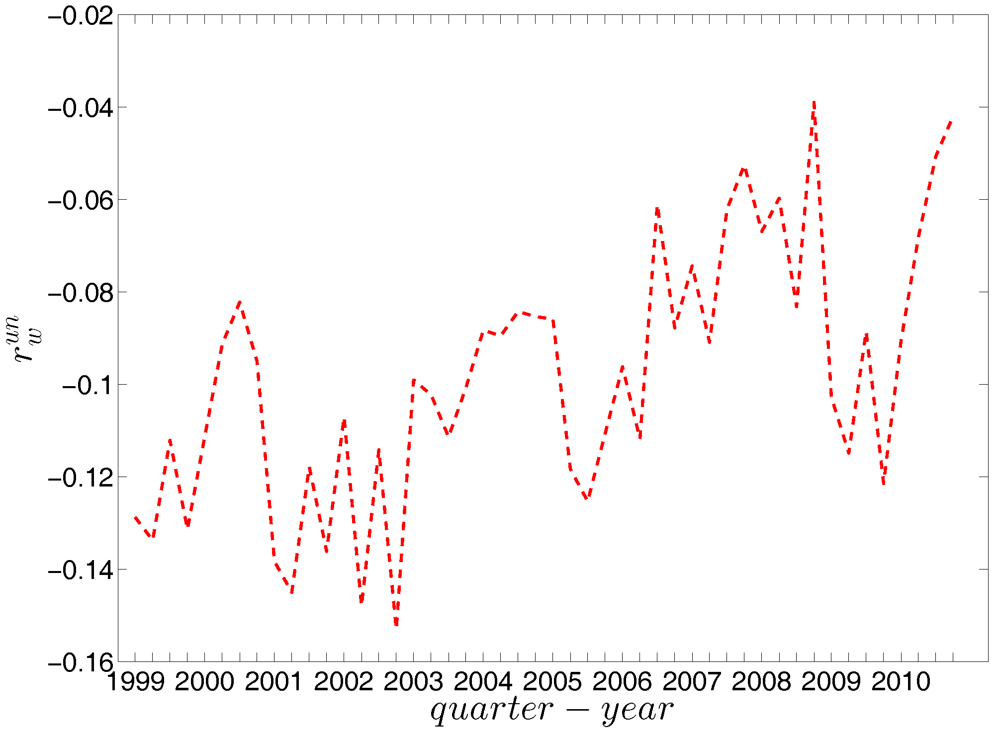
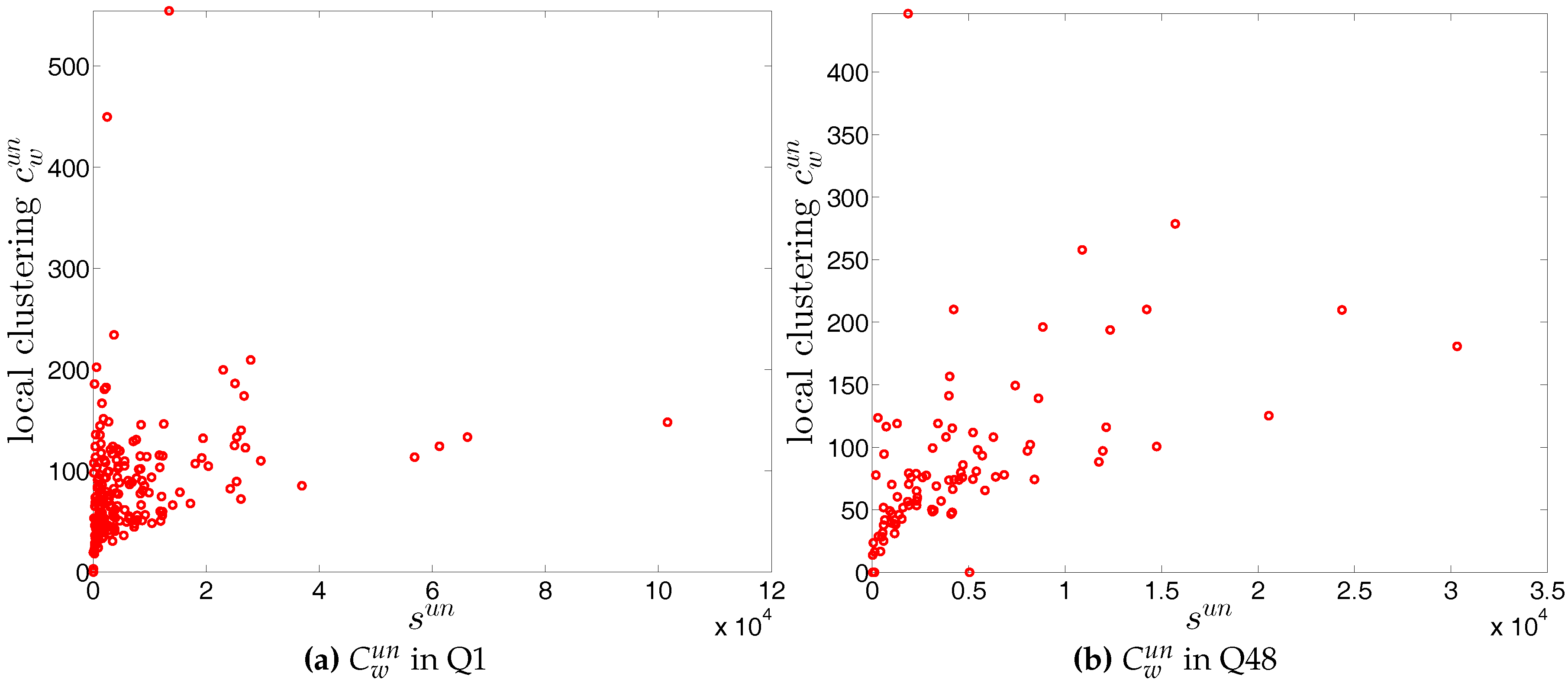
In our analysis of the third order correlations, in contrast to what we discovered in the binary version, we find that, on average banks with higher strength also have higher local clustering coefficients (see Figure 35). This is mainly because the heterogeneity in the transaction volumes across banks in every triangle is now taken into account and the average transactions of banks with high strength are much larger than those of banks with low strength. Furthermore, we observe three very distinct phases in the evolution of the average of the local weighted clustering coefficients (), i.e., before 2002, from 2002 to 2006, and from 2007 onward, which might reflect effects arising from the adoption of the euro as well as from the recent financial crisis (see Figure 36). In particular, we find that is much higher from 2002 to 2006 than in the years before and after. Notice that in the weighted version, the weighted clustering coefficients depend both on the density and on the intensity of the links in the network. During economic upswings, the network density and intensity tend to increase (as we can see in Figure 3 and Figure 4, this also happens to the e-MID network even though its size substantially declines). This leads to a higher level of weighted clustering. In contrast, during downturns, like the recent global financial crisis, banks often feel compelled to decrease both the number and the size of their credit lines (e.g., in order to create a liquidity buffer and to decrease the number of exposures), which results in lower levels of weighted clustering.
5.2. Structural Correlations in the Directed Weighted e-MID Network
In the directed weighted version of the e-MID network, we employ average nearest neighbor strength measures for the various mixing categories (), global weighted assortativity indicators (), and weighted clustering coefficients () to analyze the structural correlations.
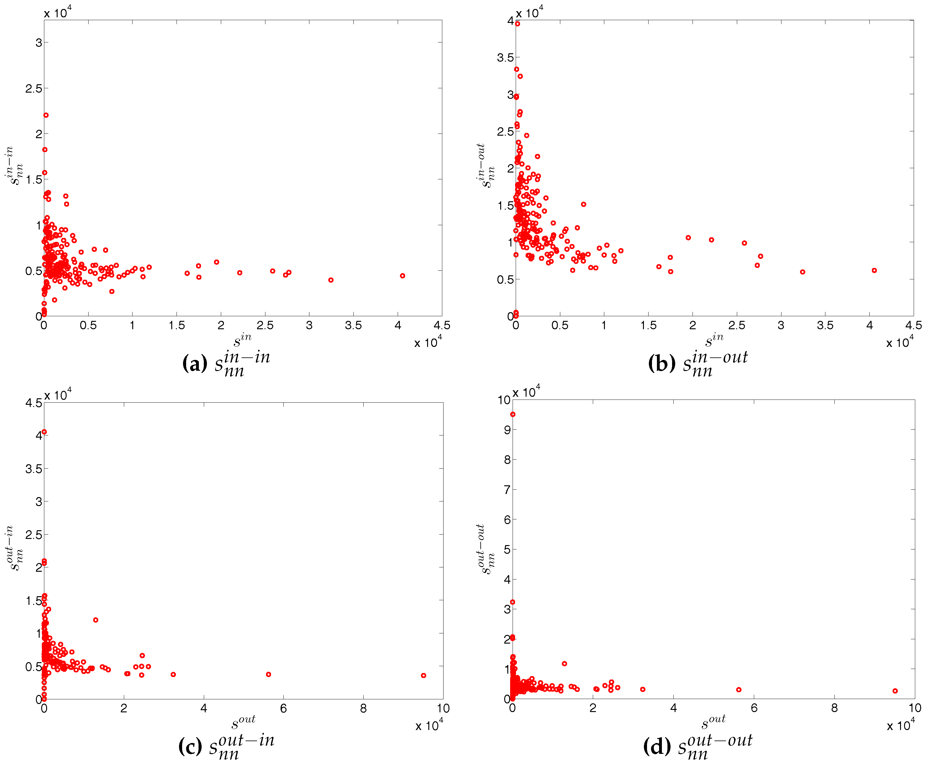
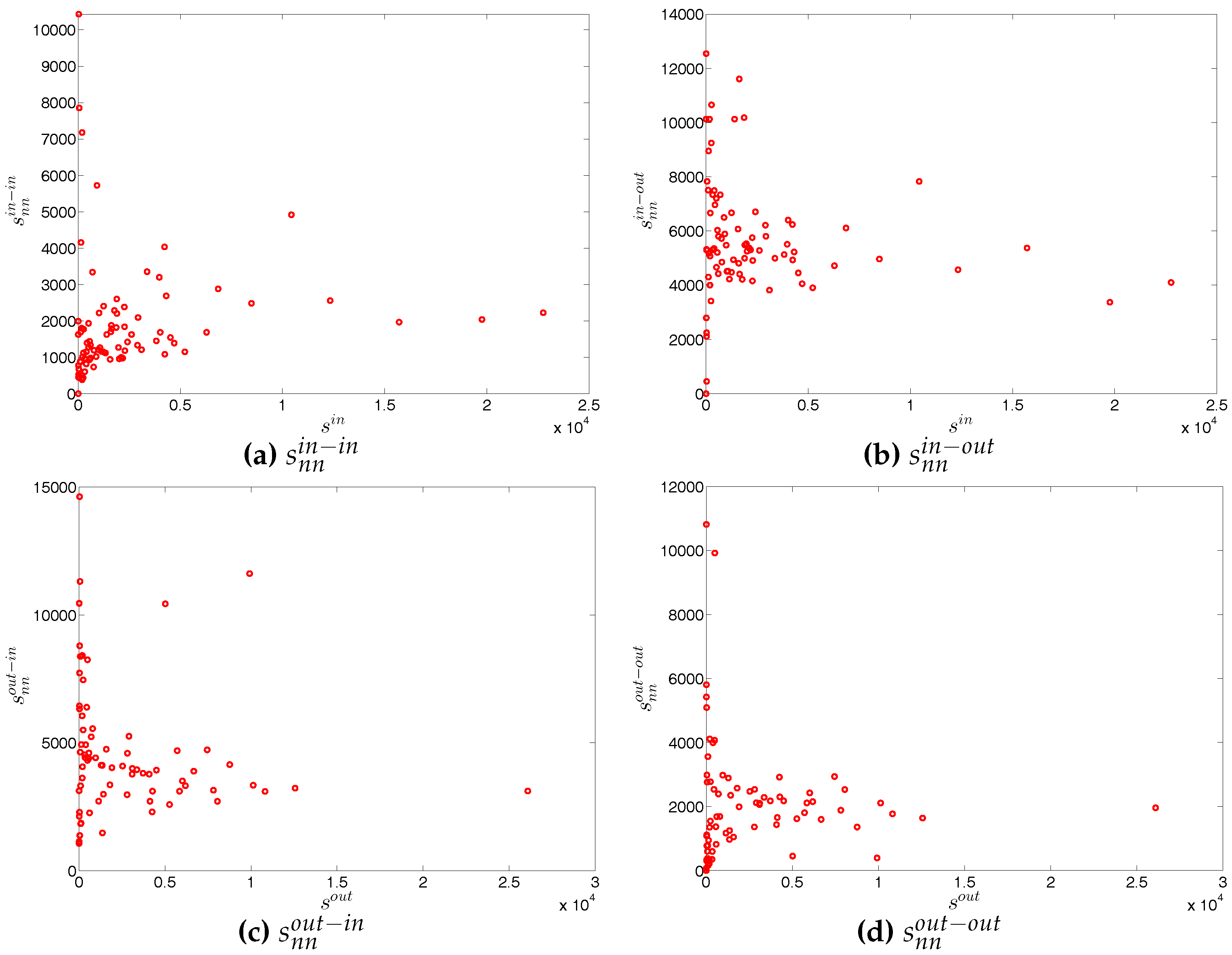
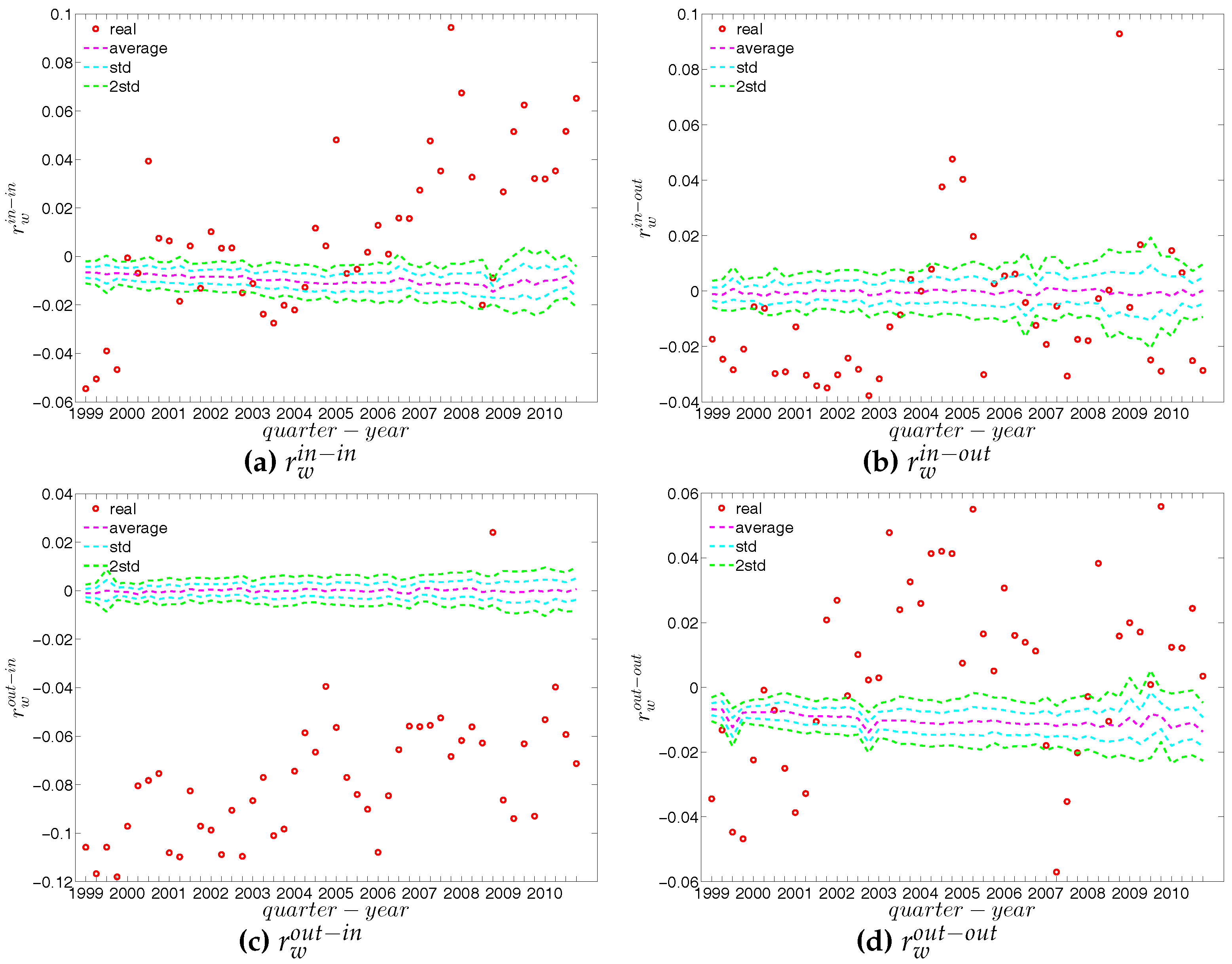
First, Figure 37 and Figure 38 show the relationship between the ANNSs and the associated strengths for all four mixing categories in Q1 and Q48. Over time, while in the first quarters, the ANNSs are a declining function of the associated strengths, in many later quarters this relationship again seems to break down, especially for the mixing categories in-in, in-out, and out-out. To obtain the overall level of strength dependency of bank interactions for each mixing category, we calculate the global assortativity indicators , and show their evolution over time in Figure 39. The results indicate that, while the out-in mixing is disassortative for the most part, the other three categories do not seem to exhibit a distinct mixing nature. In comparison to the directed binary version, the absolute values of are often smaller than those of . An interesting observation is that, among the four mixing categories, the weighted assortativity in the out-in category is closest to the undirected weighted assortativity, i.e., . For the binary versions of the network, when comparing the mixing patterns in the directed and undirected case, we made the same observation.
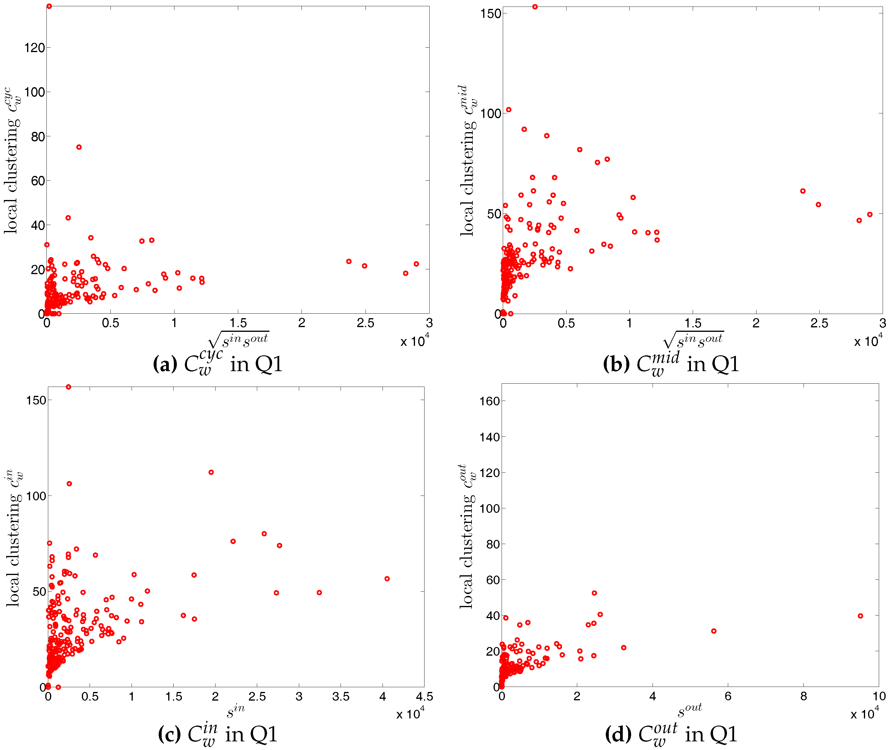
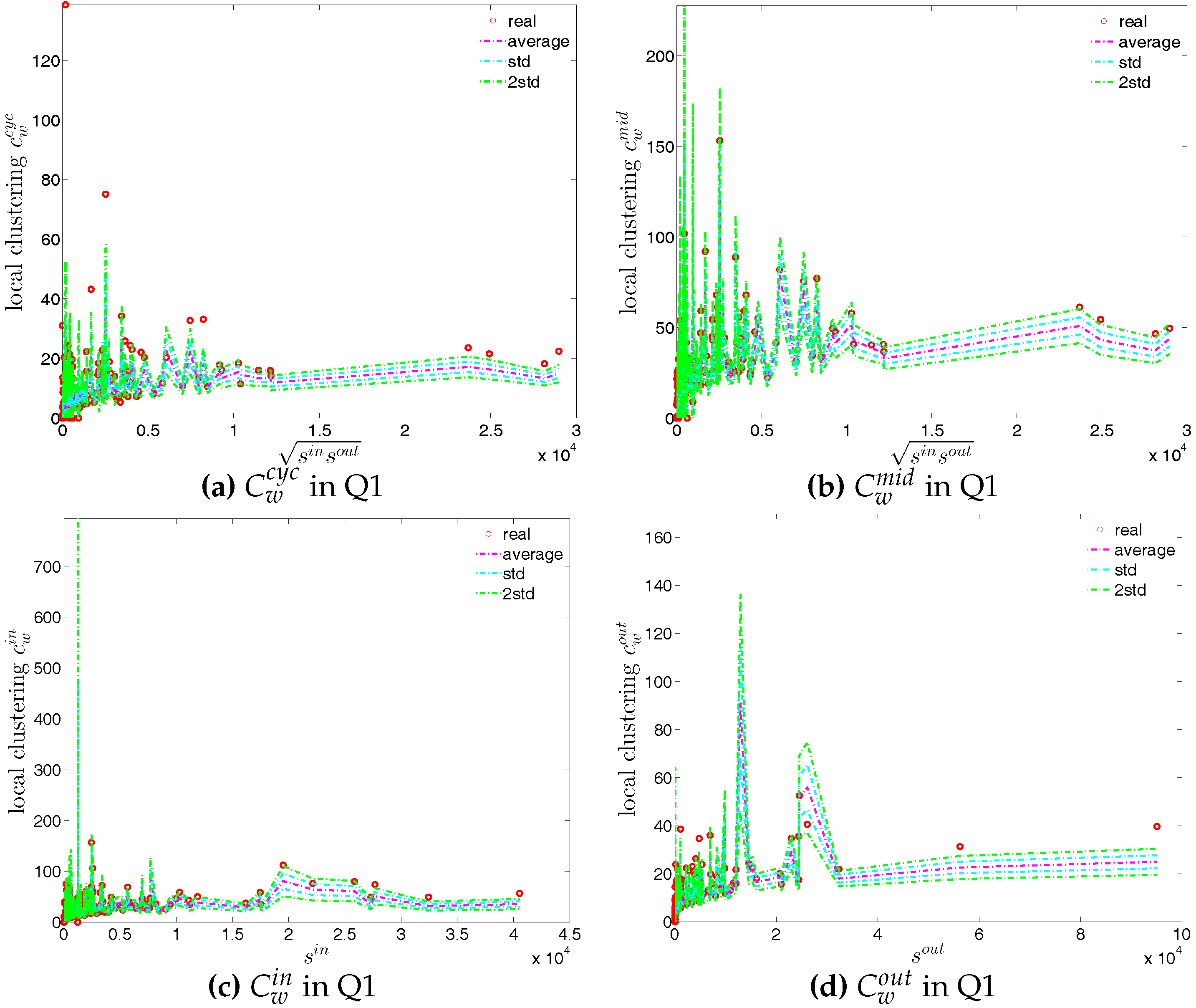
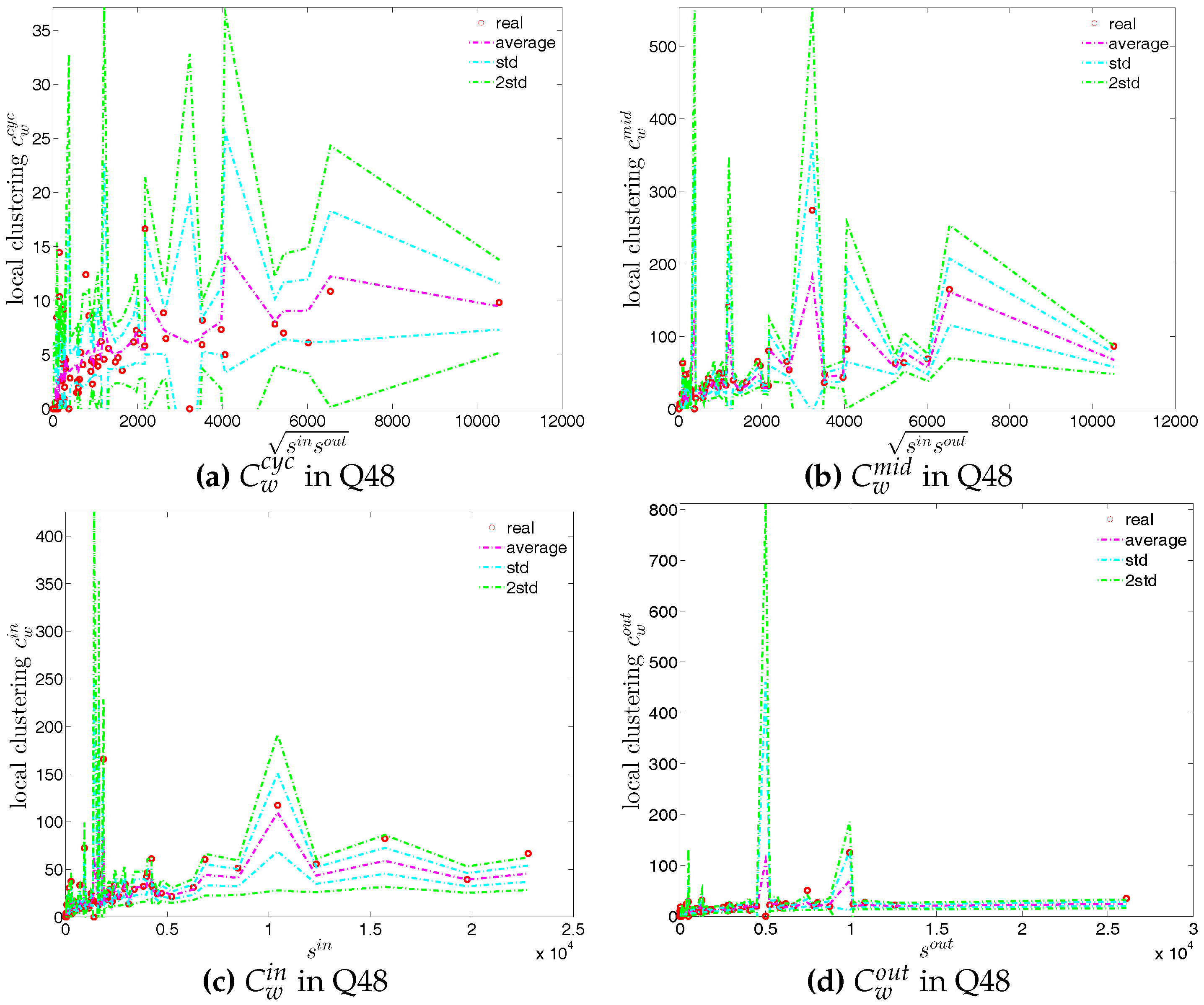
Second, the local weighted clustering coefficients for the four clustering types , , , are plotted against the associated strengths in Figure 40 and Figure 41 (in the cases of and , we plot them against ). We observe that, generally, higher (lower) strengths correspond to higher (lower) local weighted clustering coefficients.
The evolution of the averages of the local weighted clustering coefficients (i.e., , , , and , respectively for the four aforementioned types) also exhibits three different phases, i.e., before 2002, from 2002 to 2006, and from 2007 onward. For all types of clustering, the averages in the period from 2002 to 2006 are higher than those in the other two periods. Recall that, on average, larger values of , imply higher risk from concentrated funding lines, while larger values of reveal the high exposure of the associated bank to risk from defaults of their borrowers. The order and magnitude of different combinations of shown in Figure 42 thus reveal the importance of both types of risk in the period from 2002 to 2006 in the weighted version of the network. It should be emphasized that, even when all weights are normalized by the average weight over the whole network, we still observe a similar trend, signaling that the evolution of the averages of the directed local weighted clustering coefficients is not only driven by changes in the overall transaction volume (overall strength of the interactions) but also by changes in the frequency of aforementioned tripartite relations among banks.
5.3. Comparisons to the Weighted Configuration Models
5.3.1. Undirected Weighted Network
To examine the role of the heterogeneity in the local constraints for the emergence of higher order structural correlations in the weighted version of the observed network, we employ the UWCM, which preserves the observed strength sequence, and the UECM, which enforces both the observed degree as well as strength sequences onto the randomized ensemble.
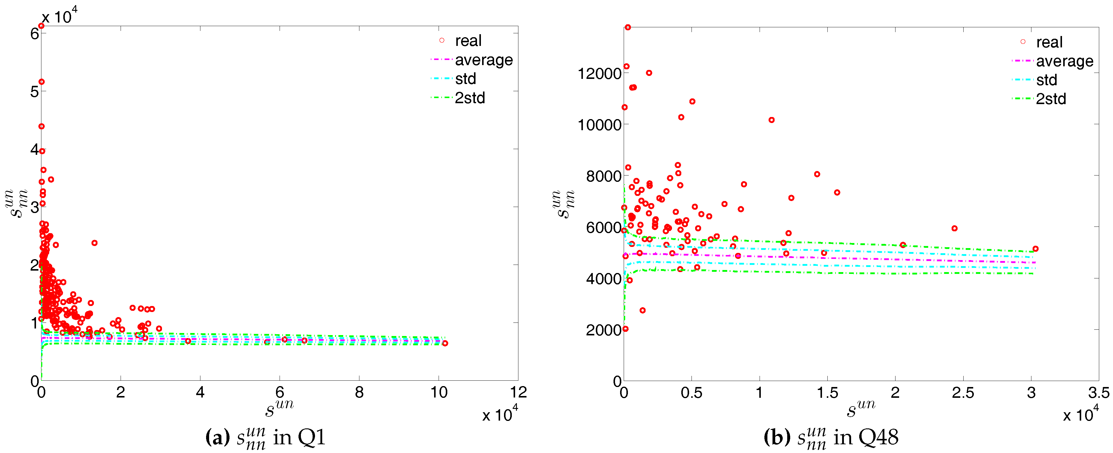
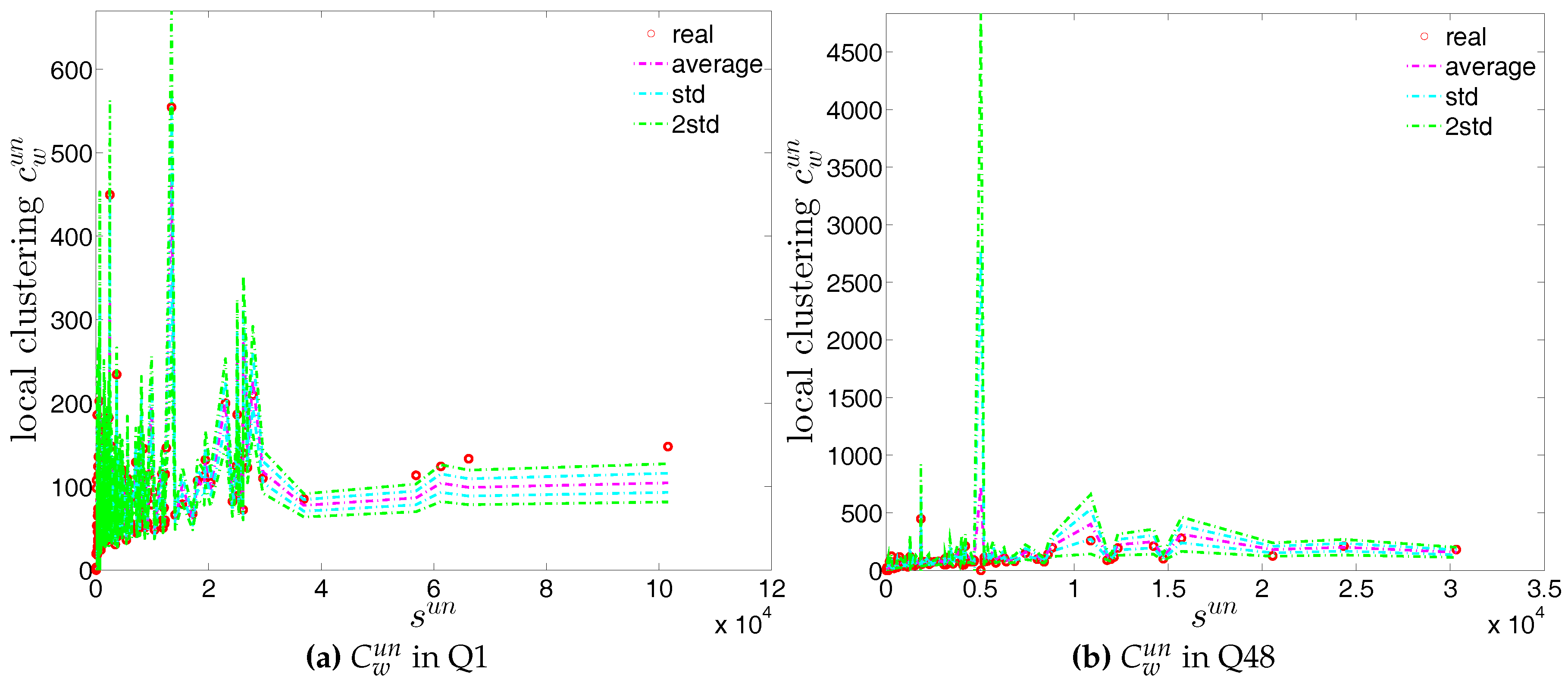
First, the observed values of the measure ANNS as well as of the local weighted clustering coefficients (as can be seen in Figure 43 and Figure 44) strongly deviate from their respective expectations under the UWCM. In contrast, we find that the UECM model is able to reproduce the main features of such measures (see Figure 45 and Figure 46).
For a more detailed comparison between the two models, we compare the z-scores of the measure ANNS as well as of the local weighted clustering coefficients evaluated under the UWCM with those for the same measures evaluated under the UECM. More specifically, for every bank i, we define the z-scores
and
where and are respectively the expected values of the measure ANNS for bank i evaluated under the UWCM and the UECM; and and are respectively the standard deviations of ANNS(i) evaluated under the UWCM and the UECM (throughout this paper, the notation and are respectively the expected value and standard deviation of X evaluated under the referenced null model).
Similarly, the z-scores for the local weighted clustering coefficients for bank i evaluated under the UWCM and the UECM are defined as
and
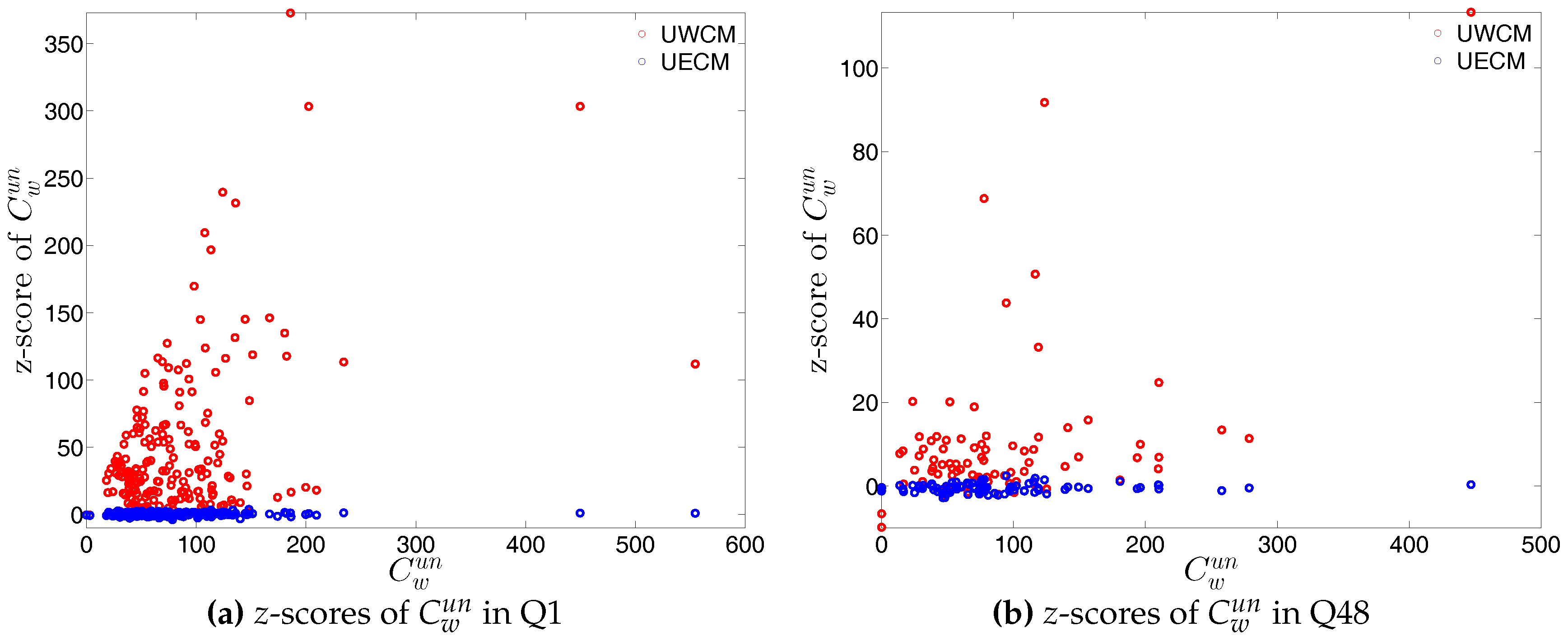
We show the comparisons between the z-scores under the two considered configuration models in Figure 47 and Figure 48. For almost all banks, we find that and .
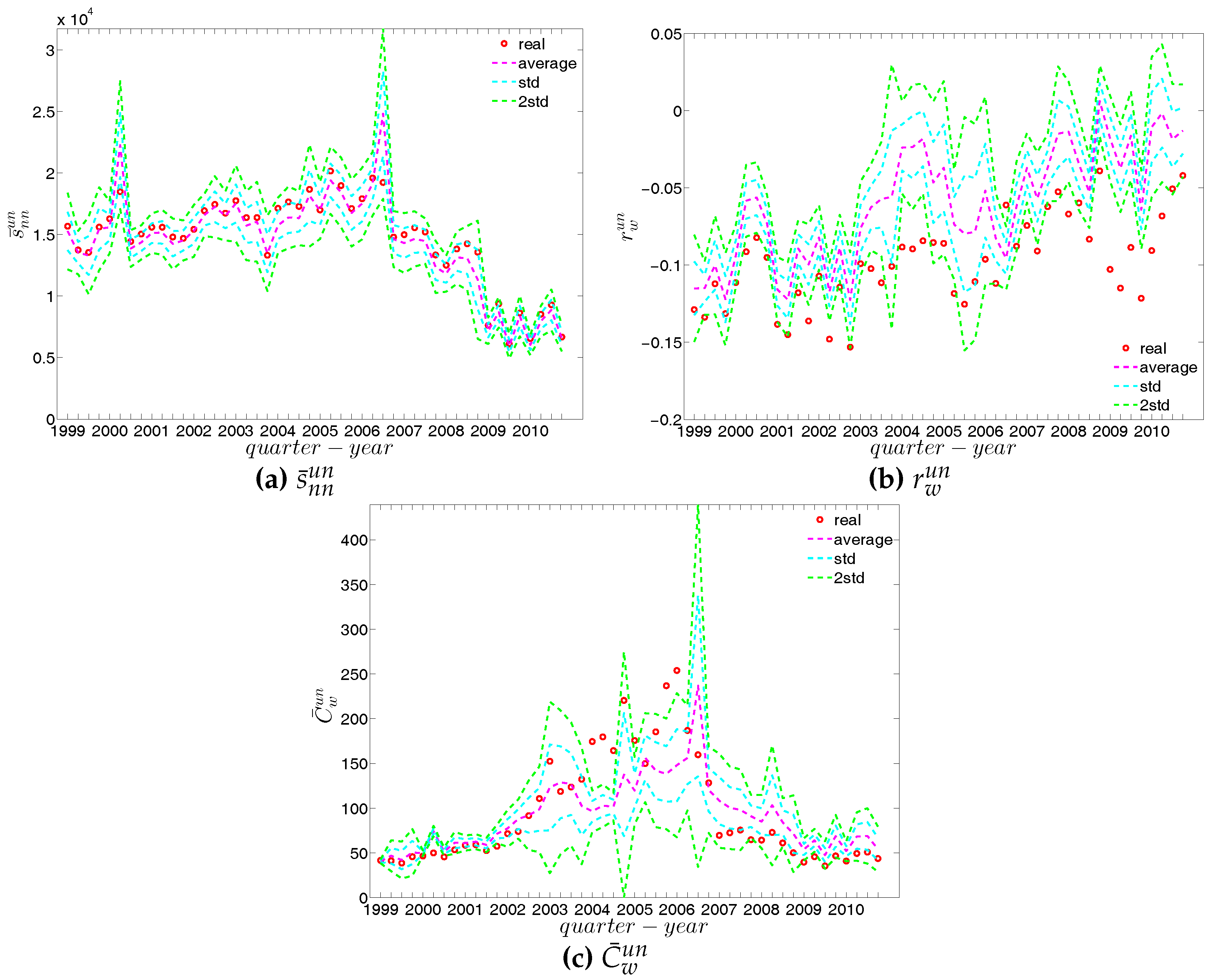
We now compare the evolution of (i.e., the average of the ANNSs over all nodes), , and for the observed network with the one obtained for these measures under the UWCM and the UECM. In Figure 49, we see that for most of the time, the observed values of , , and lie outside the ±2 bands associated with the UWCM. In contrast, in Figure 50, we see that the evolution of these measures is well captured by the ECM. The observed values of and and the expected ones obtained from the ECM are in very close agreement. Even in the case of , for which several significant deviations are found, the main features of its evolution are well reproduced by the ECM.
5.3.2. Directed Weighted Network
We now extend our comparison between the observed network and the configuration models to the directed weighted version. For this purpose, again the two relevant null models are employed, i.e., the DWCM and the DECM.
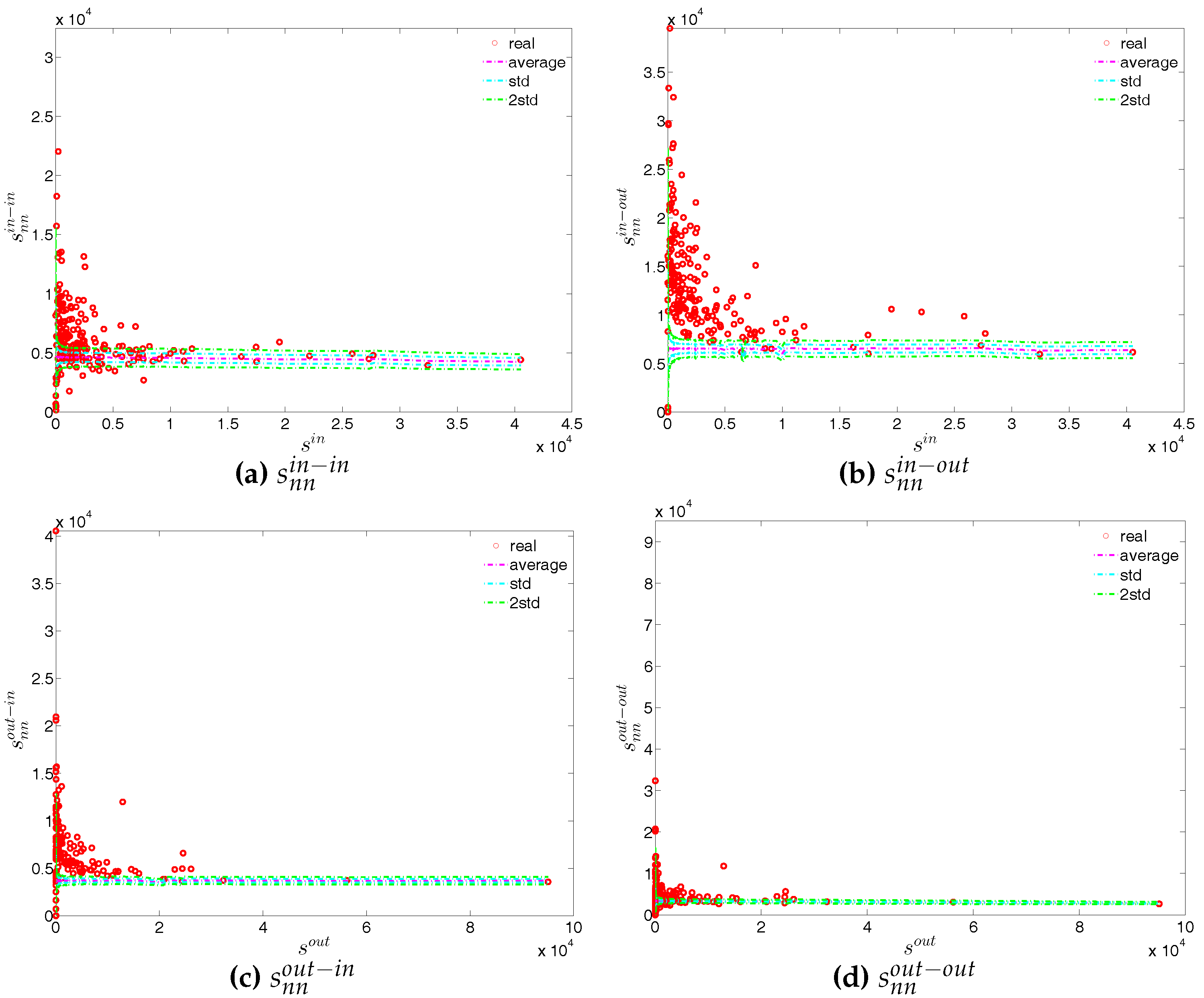
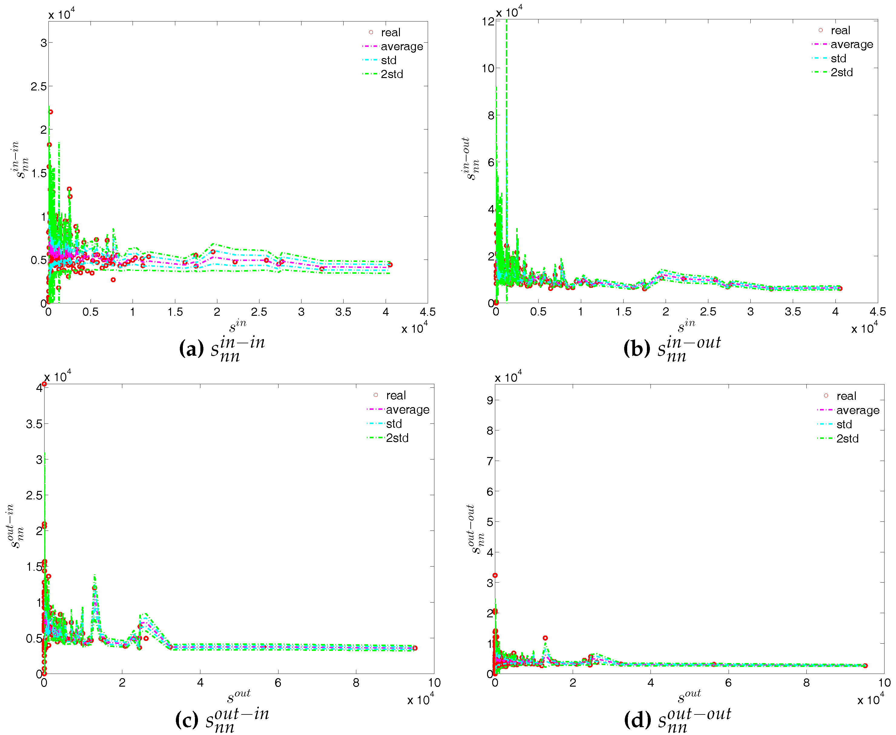
First, regarding the directed versions of the measure ANNS, we compare , , , and of the observed network in the two chosen quarters with those obtained from the DWCM in Figure 51 and Figure 52, and with those obtained from the DECM in Figure 53 and Figure 54. Similar to the undirected weighted case, the z-scores of the directed weighted versions of the measure ANNS evaluated under these two models are also reported in Figure 55 and Figure 56. Overall, we see that the main features of the measure ANNS are replicated much better by the DECM than by the DWCM. Furthermore, typically for almost all banks, we find that .
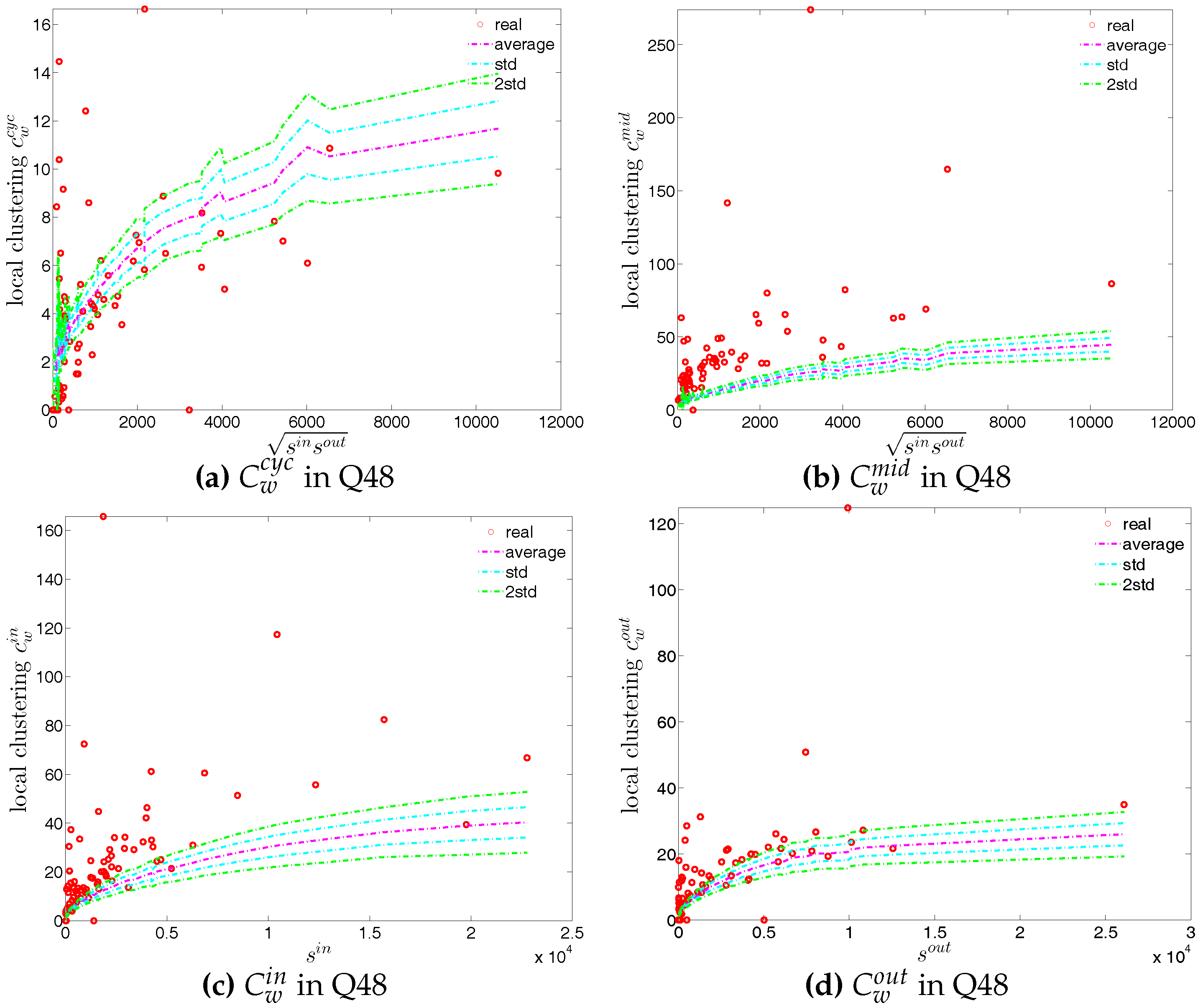
In terms of the third order structural correlations, the DECM again outperforms the DWCM in terms of reproducing the main features of local weighted clustering coefficients. This is visualized in Figure 57, Figure 58, Figure 59 and Figure 60. In addition, for each type of local weighted clustering coefficients we also calculate the z-scores evaluated under the DWCM and the DECM. As shown in Figure 61 and Figure 62, we observe that on average , , , and , although there is often a certain deviation from this general tendency at the lower end of the spectrum of degrees and strengths.
Finally, we analyze the predictive power of the two considered null models in terms of the evolution of the averages of the various versions of the measure ANNSs (i.e., , , and ), the global weighted assortativity indicators (i.e., , , and ), and the averages of the local weighted clustering coefficients (i.e., , , and ) (see also the next subsection for a further comparison).
Figure 63, Figure 64 and Figure 65 show significant deviations of the observed network from the DWCM over time. A comparison between the DECM and the observed network in terms of the aforementioned measures is shown in Figure 66, Figure 67 and Figure 68. Overall, we observe that, on the one hand, the DWCM is clearly dominated by the DECM, on the other hand, significant deviations from the DECM are still present in several quarters, regarding such as the average of the measure ANNS in the mixing category out-out (), the global weighted assortativity indicators in the in-in and in-out categories, the average of the local weighted clustering coefficients and the average of the local weighted clustering coefficients .
We emphasize that one of the main features not explained by the sequences of degrees and strengths of the network nodes themselves is the high level of clustering in the years preceding the crisis, i.e., the huge increase in various indirect exposures generated via more intensive interbank credit links. Obviously, this is the one feature that stands out in our time series. The extreme deviation of the clustering coefficient during around 2002 through 2007 from its expectation under the DWCM and DECM (and also from previous and later years) indicates some form of deliberate behavioral change of banks in this period. As it seems banks added new partners in the money market to existing ones in the boom phase but with the onset of the crisis only kept links to those partners that appeared particularly trustworthy. It seems very likely that, banks might have seen little risk in short-run interbank loans and, therefore, they had increased their range of trading partners, while with the emerging awareness of severe risk of failures of counterparties, they restricted their transactions to those counterparties to whom a strong bilateral relationship had been built up. Again, this conclusion is supported by the behavioral model estimated by [41].
Note that, although, in general, we find that the family of Enhanced Configuration Models outperforms the family of Weighted Configuration Models in terms of replicating the main features of the structural correlations in the weighted version of the observed network, solving the system (29) to extract the hidden variables in the DECM (or system (25) in the UECM for the undirected version of the network) is much more computationally demanding than solving the system (23) for the DWCM (or system (19) for the UWCM for the undirected version of the network). According to [13], solving for hidden variables under Enhanced Configuration Models may be very time consuming if the strength distribution contains big outliers and the degree distribution is narrow. Indeed, our data set shows that the strength distribution is much wider than the degree distribution. Following [13,17], in order to speed up the process of solving systems (25) and (29), we have used the iteration method, which uses the output of the previous iteration as the initial value for the current one. However, it remains a very time consuming process to obtain an acceptable solution for the hidden variables.
Since the Enhanced Configuration Model uses both the information on the degree sequence and the weight sequence in the data, it is not too surprising that it should perform better than theWeighted Configuration Model. Too highlight the difference between both approaches, we show in Appendix B the expected link probabilities and expected weights computed from the estimated hidden variables under all models. As it transpires, link probabilities have quite some right-hand skewness when computed on the base of weight sequences only. The model would, thus, predict existence of links with a probability close to one for those nodes that have the highest strength (volume). Hence, the negligence of the degree sequence brings in some tendency towards assortativity that is in contrast to the empirical behavior of the underlying data. Since the Enhanced Configuration Model keeps the degree distribution together with the distribution of weights it does not suffer from such a bias, and hence can generate an ensemble of networks that better accommodates this stylized fact.
5.4. z-Scores Analysis Revealing Structural Changes in the Weighted System
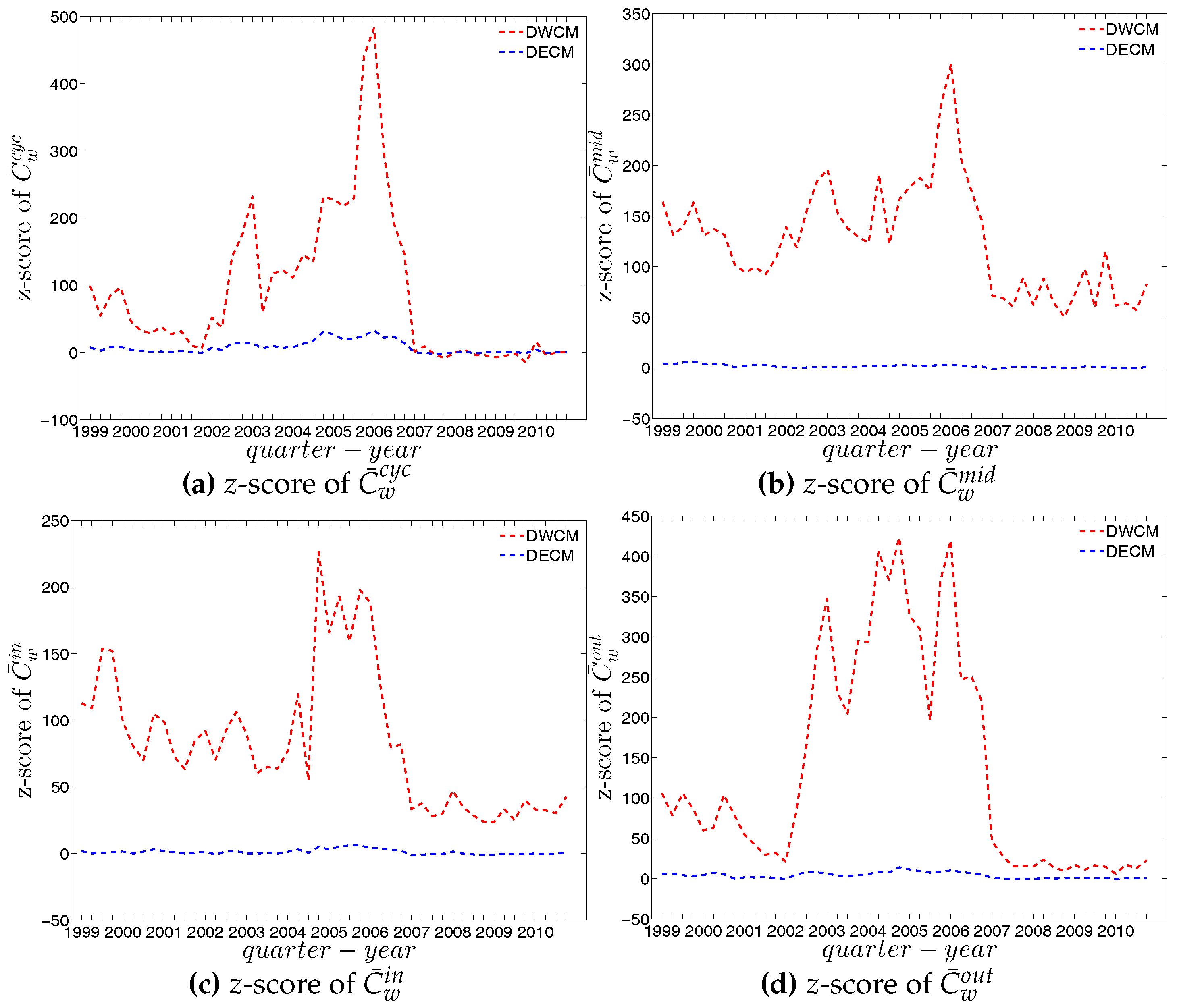
To analyze the evolution of the discrepancies between the referenced models and the observed network, we define z-scores for the global indicators, i.e., for in the undirected weighted network (evaluated under the UWCM and the UECM) and for , , , and in the directed weighted network (evaluated under the DWCM and the DECM).
Before going into details, it should be noted that from Figure 69, Figure 70, Figure 71 and Figure 72, when comparing the UECM with the UWCM in the undirected version or the DECM with the DWCM in the directed version, some of the high z-scores under the UECM (or under the DECM) are blurred because of the presence of much larger z-scores under the UWCM (or under the DWCM).
In the undirected weighted case, two important findings are obtained. First, overall, the z-scores are mostly smaller in absolute value under the UECM than under the UWCM (see Figure 69). This is consistent with what we found for the local indicators and underlines the general finding that the UECM out-performs the UWCM. Second, interestingly, in Figure 69c we see that the distance between the z-scores for evaluated under the UWCM and the UECM increases over the period from 2002 to 2006, and then decreases sharply after the financial crisis. This suggests that the importance of particular basic features of a network (like its degree sequence or its strength sequence) for the emergence of higher order correlations structures can vary over time.
In the directed weighted case, similarly, we find that the z-scores under the DECM are much smaller in absolute value than those evaluated under the DWCM (see Figure 70, Figure 71 and Figure 72). As we can see in Figure 72, similar to the undirected version, the distance between the z-scores for each of the evaluated under the DWCM and the DECM continuously increases during the period 2002 to 2006, and then decreases dramatically after the financial crisis.
6. Conclusions
In this study, we have investigated the structural correlations in the e-MID network. We find that the observed structural correlations can vary across different versions of the network (binary vs. weighted and undirected vs. directed). In the undirected version of the network, the mixing is disassortative in both the binary and the weighted case. In addition, when the directions of the edges are taken into account, we find that among the four mixing categories (i.e., in-in, in-out, out-in, and out-out), the global assortativity in the out-in category comes closest to the mixing observed in the undirected network. The similarity between these two quantities is suggested by [34]. Due to the fact that only in the out-in mixing category the considered edge (see the out-in category in Figure 1) contributes to the node degrees on both of its sides, this mixing category can be considered a generalization of the mixing in undirected networks. During our analysis of the evolution of the third order correlations among banks over time, we detected dramatic changes in the network structure surrounding the recent financial crisis in 2007. More specifically, in the weighted network, the averages of the local weighted clustering coefficients appear elevated from the adoption of the Euro up until 2006, and then decrease dramatically around the time of the financial crisis. We also report strong indications of elevated shared risk in the network, evidenced by the prevalence of the “middleman” and “inward” types of clustering in the network.
Moreover, by employing the various configuration models, we examined whether the information encoded in the local constraints (like the observed degree sequence and/or the strength sequence of a network) can explain higher order structural correlations. We find that, in the binary case, the degree sequence is informative in terms of explaining the main features of the structural correlations in the e-MID network. However, under closer scrutiny, the binary e-MID network does display some patterns that cannot simply be explained by the degree sequence in conjunction with the configuration model.
In the weighted version of the network, for the most part, the structural correlations in the observed e-MID network are deviating strongly from their respective expectations evaluated under the Weighted Configuration Models, which capture only the heterogeneity in the strength sequence(s) (i.e., the UWCM in the undirected version and the DWCM in the directed version). One possible explanation is that while all measures of structural correlations used in the weighted network depend on the elements of both the adjacency as well as the weighting matrices, neither the UWCM or DWCM utilize information about the node degrees (degree sequence), which is, in fact, found to be more important than the strength sequence in reproducing the topological properties of real world networks (see, for example, [13,15,16]).
Due to the failures of the UWCM and the DWCM, we consider the family of Enhanced Configuration Models, which constrains the degree as well as the strength sequences of the randomized ensemble to match those of the observed network on average (i.e., UECM in the undirected case and the DECM in the directed case). Our findings indicate that the randomized ensembles produced by the Enhanced Configuration Model have a much greater predictive power. This is in line with what was found in previous studies such as [13,17], and is not very surprising since the Enhanced Configuration Models utilize more information when replicating the structural correlations of the observed network. The results obtained from the analysis of the DECM confirms the role that the distribution of the in-coming and out-going degrees together with their strengths (volumes) in directed weighted networks plays for the emergence of higher order structural correlations.
Still, a detailed comparison between the observed network and the Enhanced Configuration Models reveals that even this family of Configuration Models is not able to produce accurate estimates for all the measures of structural correlations we used, meaning that some of the patterns can be considered non-random or unexplained by the models. For instance, in the undirected network, we find that even when using the UECM, the weighted assortativity deviates significantly from the respective expected value in a couple of times. In the directed weighted network, the global weighted assortativity in the in-in as well as in the in-out mixing categories and the average of the local weighted clustering coefficients of “inward”, “outward”, and “cyclical” clustering also display patterns in several quarters, mainly from 2002 to 2006, that deviate from the expectations based on the configuration model. The high degree of clustering in this episode is the one characteristic that can not be explained satisfactorily via the influence of lower-order characteristics like the degree and strength sequences. Hence, this finding points to a behavioral change in the formation of the credit network: A deliberate increase of indirect exposure through multiple credit relations. Interestingly, with the crisis year 2007, we find an abrupt reduction of all clustering coefficients to their “normal” levels implied by the degree and strength sequences.
The Enhanced Configuration Models also fail to reproduce the local behavior of certain banks captured by the local indicators of structural correlations. Unfortunately, because of the lack of more detailed information about the banks in the system, we can not identify the factors for the formations of such deviating patterns.
Interestingly, similar to the study of [36], we also observe evidence for structural changes when comparing the weighted version of the e-MID network with the weighted configuration models. Squartini et al. [36] focuse on the analysis of the binary version of the network of interbank exposures among Dutch banks over the period 1998–2008. More specifically, the distance between the predictions of the Weighted Configuration Models and of the Enhanced Configuration Models for the averages of local weighted clustering coefficients continuously increases from the adoption of the Euro up until the financial crisis in 2007 and then sharply decreases after that. This result can be interpreted as an indication of structural changes in the network associated with these two critical events. It also suggests that the importance of particular basic features of a network (like its degree sequence or its strength sequence) for the emergence of higher order correlation structures can vary over time.
Due to issues of confidentiality, in many cases, the biggest challenge in the analysis of complex financial systems lies in the utilization of the limited available information. Our results can be understood as an evaluation of the potential of configuration models to reconstruct higher order topological properties of a network from limited information (e.g., see [17,24]). Meaningful systemic risk evaluation can be conducted on reconstructed networks only to the extent to which the reconstruction is reliable (see, for example, [43]).
In addition, the configuration models translate the local constraints in the observed network into hidden variables associated with the individual banks. It would be interesting to investigate whether some individual node characteristics (i.e., non-topological properties like bank’s size and leverage) correlate with the extracted hidden variables (see, for example, [14,44,45,46]), however, such additional information is unfortunately not available in our data set. This can be a fruitful direction for future research into financial networks.
Moreover, since the Exponential Random Graph Model is generic and flexible enough, one may want to investigate the extent to which it can be useful to use other statistics of the observed network as ensemble constraints. For instance, the average degree of the nearest neighbors or the local clustering coefficients might also prove informative in explaining particular topological properties of the observed network (see, for example, [35,47] for employing different constraints). In addition, since the second and third order structural correlations are the main focus of this study, we suggest that the role of various constraints for the emergence of higher order correlations (or motifs) and for the meso-scale network structures such as the core-periphery and community structures should be studied further.
Author Contributions
All authors contributed equally to this article.
Conflicts of Interest
The authors declare no conflict of interest.
Appendix A
Appendix A.1. Overall Assortativity
In an undirected network, define the list of m edges , where for each index e, the two nodes stand for the ends of an edge. Note that, the overall assortativity indicator can be calculated via and as
where (e.g., [48]).
In a directed network, suppose that we have a list of M edges , where for each index e, the two nodes respectively stand for the source and target nodes (note that ).
Each node or has an in-coming degree and an out-going degree (see Figure A1). Consequently, we have four combinations of degrees associated with each edge as mentioned in Figure 1. Therefore, regarding the degree dependencies, four separate indicators can be obtained, i.e., . Similar to the undirected case, mathematically, these measures of overall assortativity actually depend on the degree sequences , as well as the sequences of the average nearest neighbor degrees (e.g., [33,34]). More specifically, accordingly, they are given by
and
Figure A1.
In-coming, out-going degrees to two vertices of an edge in directed networks.

Appendix A.2. Local Assortativity
The local assortativity statistics is obtained as the (unbiased) contribution of individual nodes to the overall (global) assortativity. The basic idea is that the numerator in the Pearson correlation coefficient proposed by [26] can be reformulated based on the contribution of individual nodes instead of edges (e.g., [33,38]).
It should be emphasized that, for the directed version of the measure of local assortativity introduced in [33], the two in-out and out-in degree dependencies are not differentiated, when in fact they exhibit totally different behaviors (as found in [32] and in Section 4 of our study). In our study, the contributions to the in-out and out-in degree dependencies are distinguishable.
We denote the local assortativity measures for a given node i as , , , and corresponding to the four mixing categories in the directed version and is used for the undirected version. Note that the following equalities must hold:
First, we define
and
Note that, in the undirected case, it can be shown that is equal to the average of the degrees of the target and source nodes in the edge list , i.e., . Similarly, in the directed case, given the edge list , it can be shown that and are respectively equal to the averages of the in-coming and out-going degrees from target and source nodes in the edge list. Mathematically, and . In contrast, () gives the average of out-going (in-coming) degrees of the target (source) nodes in the edge list. We have that and .
Second, we define
and
By decomposing the overall assortativity coefficient in Equation (A1), we obtain the local assortativity indicators. More specifically, the contribution of node i to r is
Similarly, in the directed case, for each node i, we have four local assortativity indicators:
Appendix B
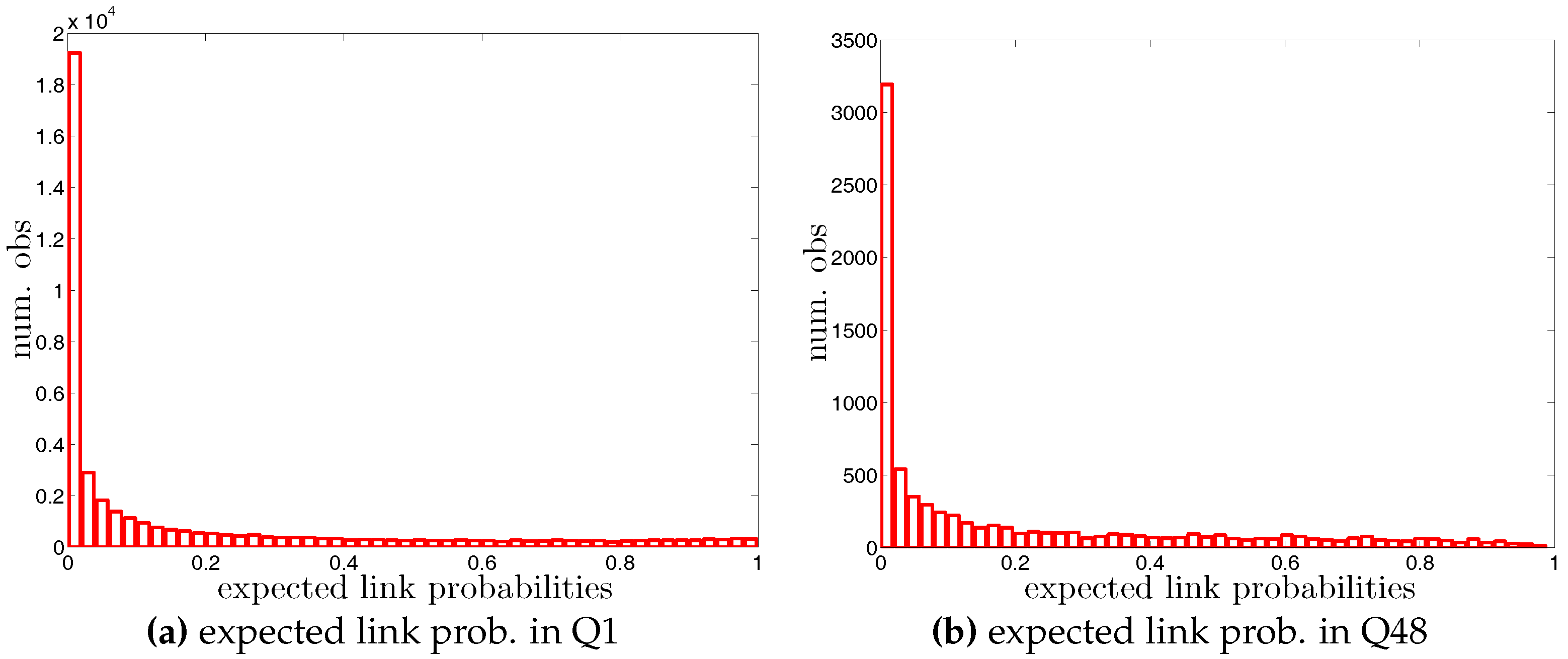
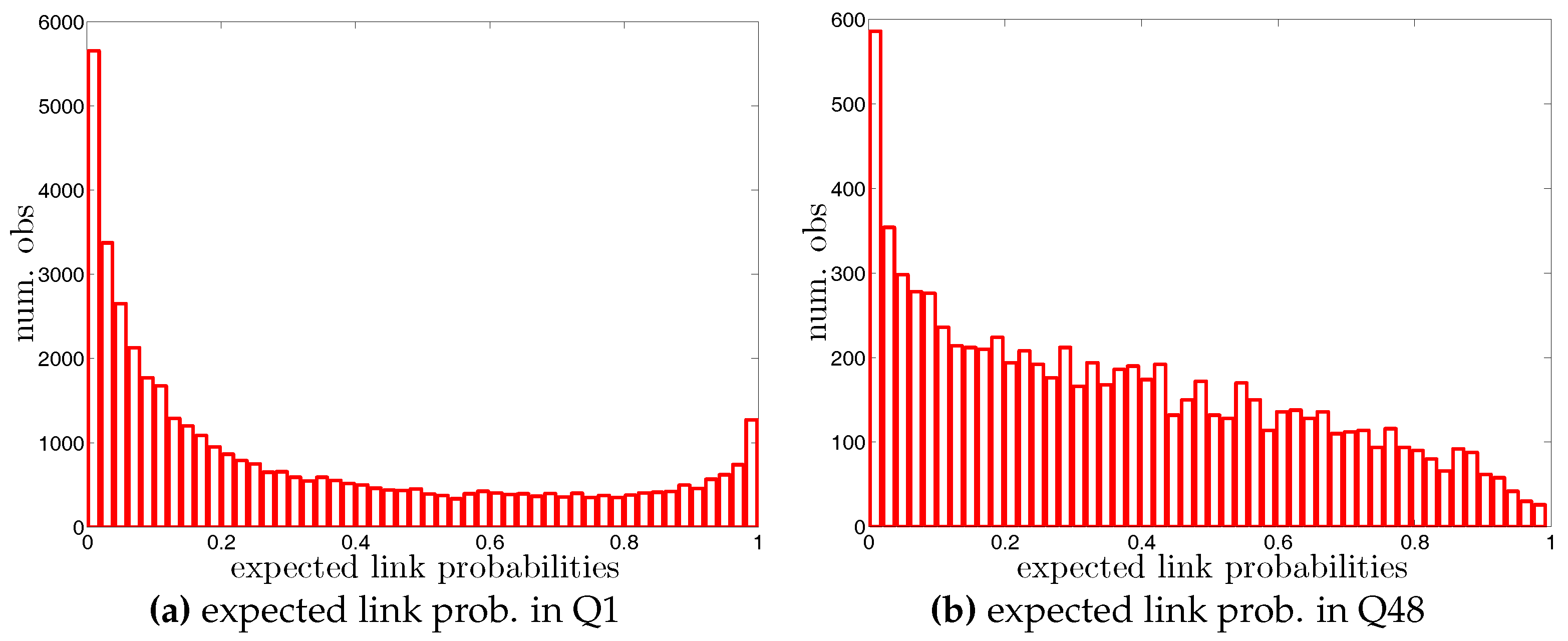
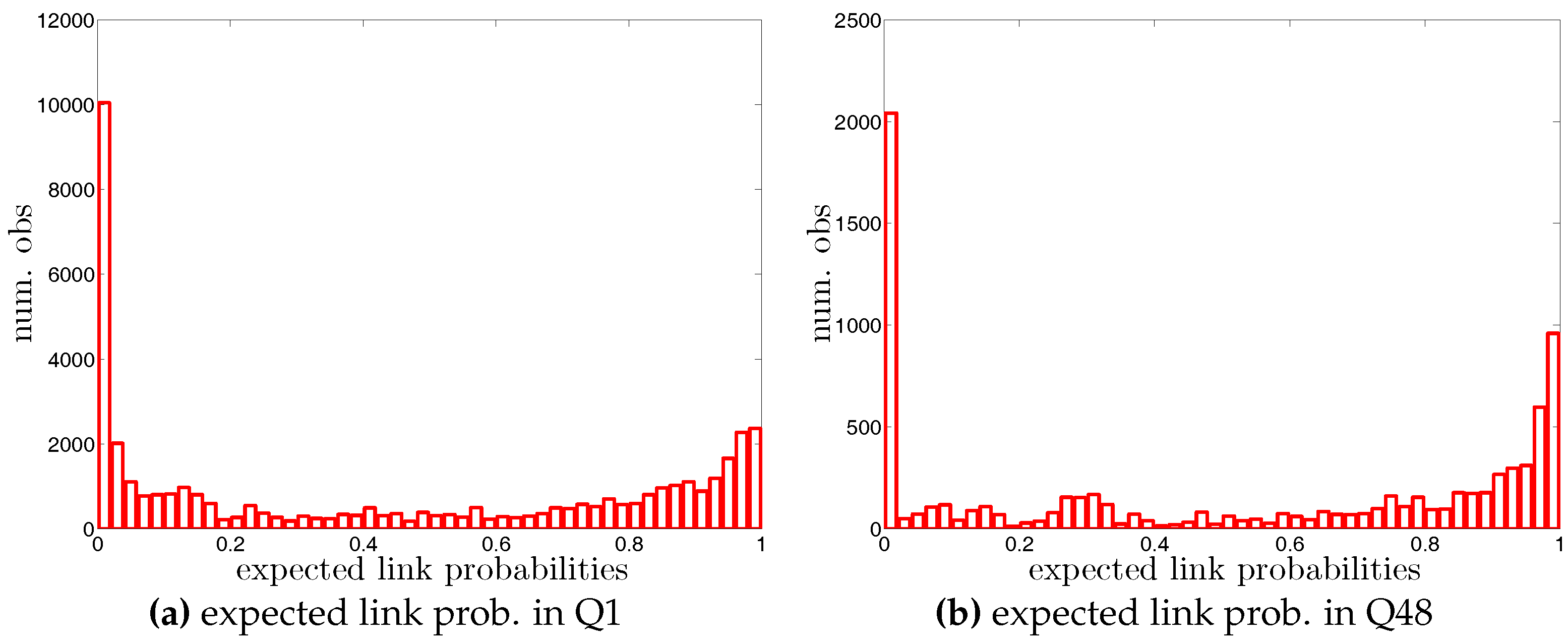
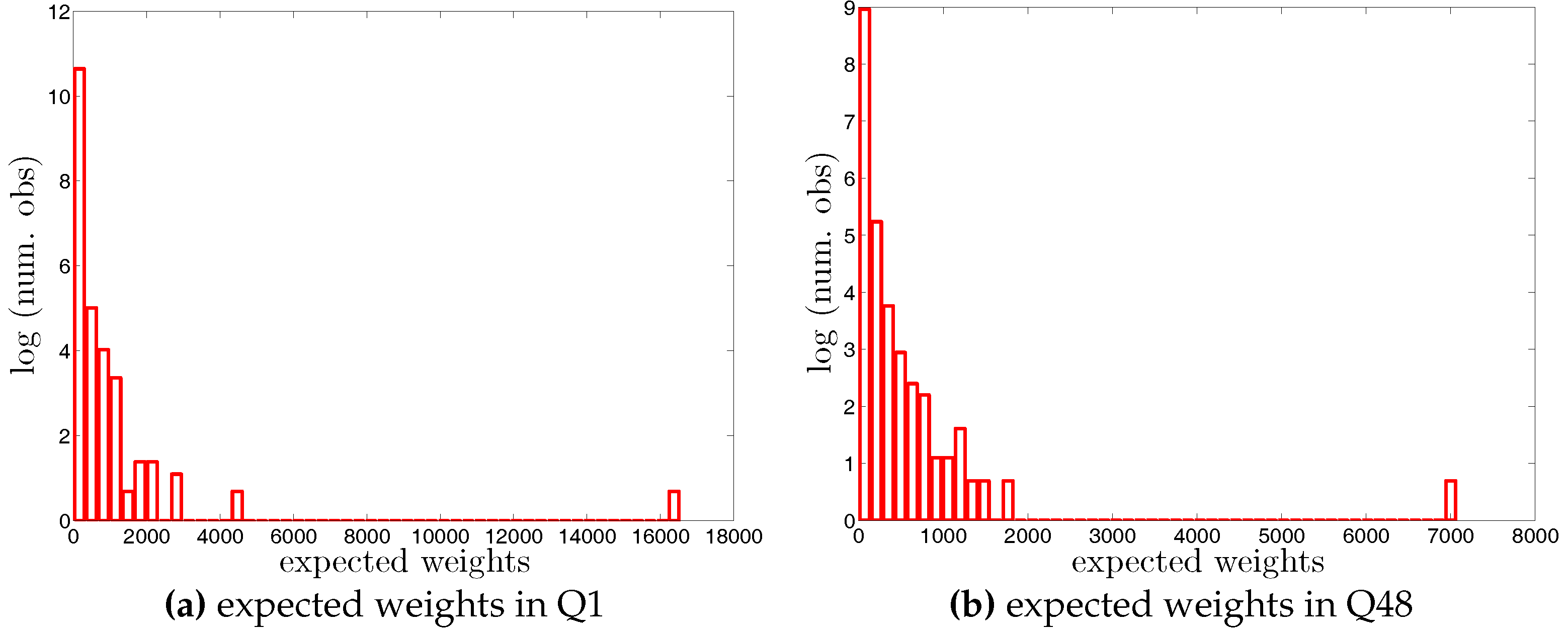
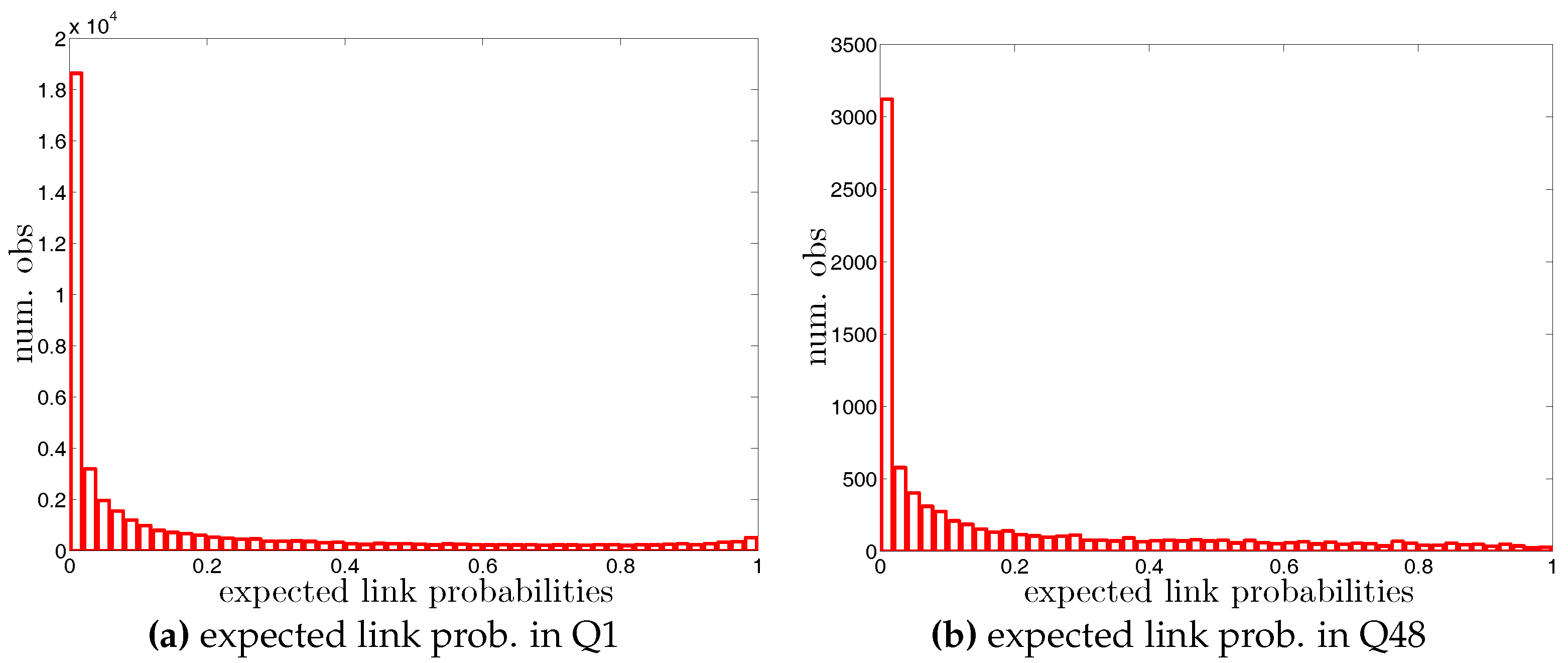
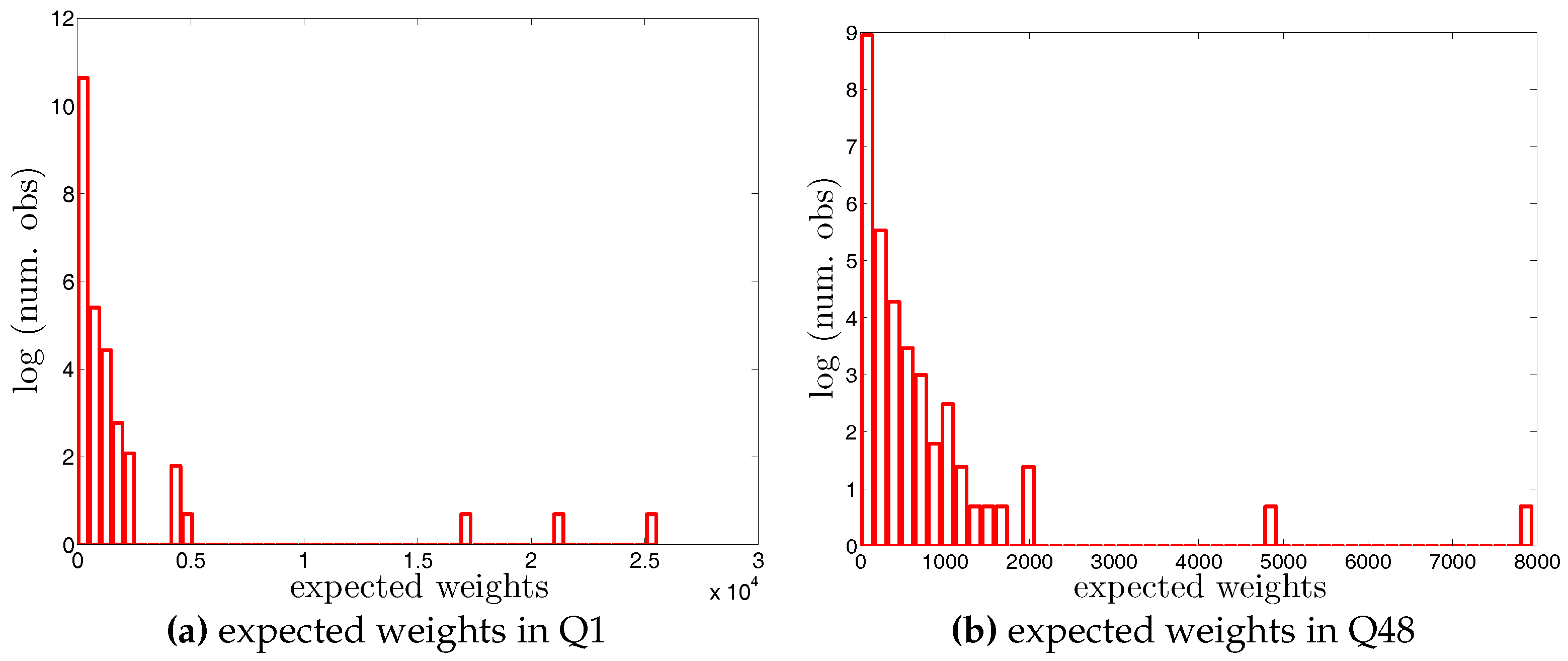
In the followings, we will provide the distributions of expected link probabilities (i.e., for every pair of different nodes i and j) and weights (i.e., for every pair of different nodes i and j) under the different configuration models, i.e., the UBCM and DBCM in the binary version, the UWCM, UECM, DWCM, and DECM in the weighted version (see Section 2.3 in the main text for details). Again, for the sake of conciseness, here we only report the results for the two quarters, Q1 and Q48.
As mentioned in Section 2 of the main text, under the UBCM and DBCM we only obtain the expected link probabilities, while under the UWCM, UECM, DWCM, and DECM we obtain both the expected link probabilities as well as the expected weights. Note that under the UBCM and DBCM in the binary version, depends on hidden variables extracted from the observed degrees. For the weighted version of the network, under the UWCM and DWCM, and depend on hidden variables extracted from the observed strengths, while under the UECM and DECM, and depend on hidden variables extracted from both the observed degrees as well as strengths.
• Distributions of Expected Undirected Link Probabilities under the UBCM
Figure A2.
Histogram of expected undirected link probabilities, , under the UBCM in Q1 and Q48.

• Distributions of expected directed link probabilities under the DBCM
Figure A3.
Histogram of expected directed link probabilities, , under the DBCM in Q1 and Q48.

• Distributions of Expected Undirected Link Probabilities and Weights under the UWCM
Figure A4.
Histogram of expected undirected link probabilities, , under the UWCM in Q1 and Q48.
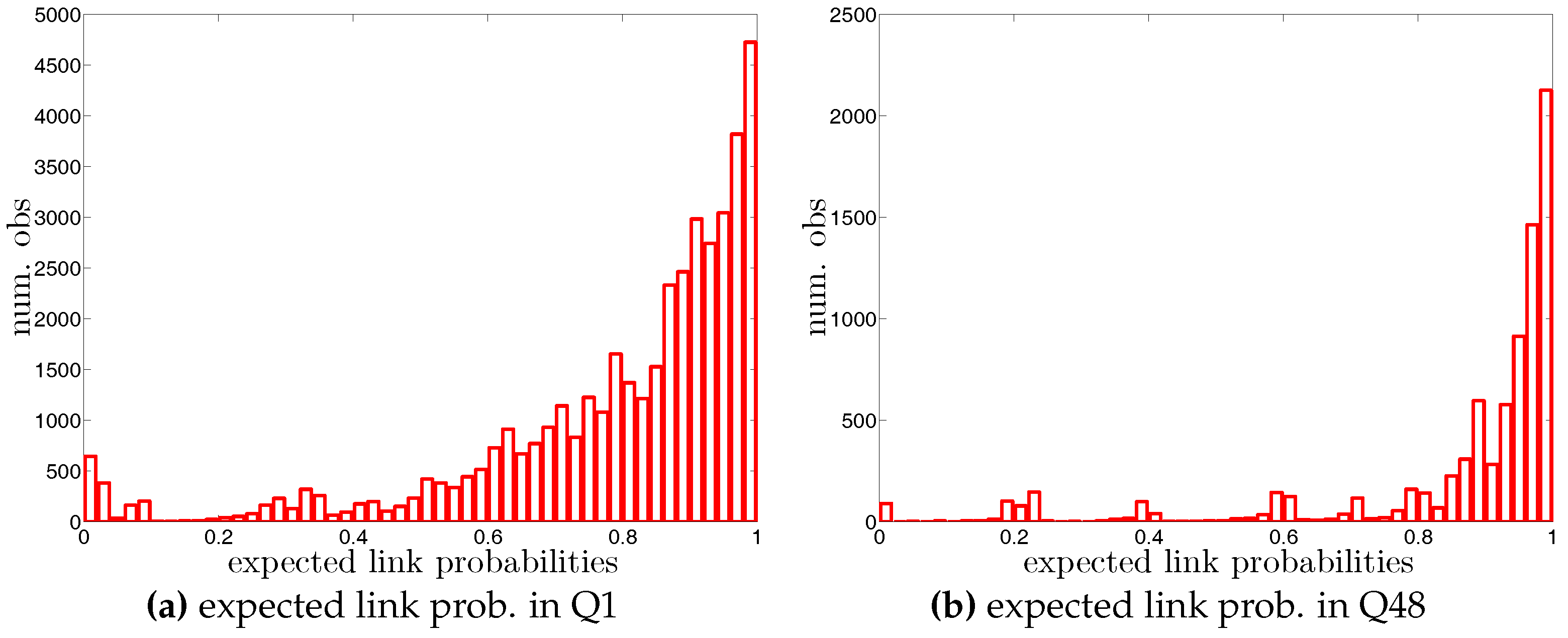
Figure A5.
Histogram of expected undirected weights, , under the UWCM in Q1 and Q48. Note that for the sake of readability, we plot the number of the observations in log scale.
Figure A5.
Histogram of expected undirected weights, , under the UWCM in Q1 and Q48. Note that for the sake of readability, we plot the number of the observations in log scale.
• Distributions of Expected Undirected Link Probabilities and Weights under the UECM
Figure A6.
Histogram of expected undirected link probabilities, , under the UECM in Q1 and Q48.

Figure A7.
Histogram of expected undirected weights, , under the UECM in Q1 and Q48. Note that for the sake of readability, we plot the number of the observations in log scale.
Figure A7.
Histogram of expected undirected weights, , under the UECM in Q1 and Q48. Note that for the sake of readability, we plot the number of the observations in log scale.
• Distributions of Expected Directed Link Probabilities and Weights under the DWCM
Figure A8.
Histogram of expected directed link probabilities, , under the DWCM in Q1 and Q48.

Figure A9.
Histogram of expected directed weights, , under the DWCM in Q1 and Q48. Note that for the sake of readability, we plot the number of the observations in log scale.
Figure A9.
Histogram of expected directed weights, , under the DWCM in Q1 and Q48. Note that for the sake of readability, we plot the number of the observations in log scale.

• Distributions of Expected Directed Link Probabilities and Weights under the DECM
Figure A10.
Histogram of expected directed link probabilities, , under the DECM in Q1 and Q48.

Figure A11.
Histogram of expected directed weights, , under the DECM in Q1 and Q48. Note that for the sake of readability, we plot the number of the observations in log scale.
Figure A11.
Histogram of expected directed weights, , under the DECM in Q1 and Q48. Note that for the sake of readability, we plot the number of the observations in log scale.
References
- Allen, F.; Gale, D. Financial contagion. J. Political Econ. 2000, 108, 1–33. [Google Scholar] [CrossRef]
- Haldane, A. Rethinking the Financial Network. Available online: http://www.bis.org/review/r090505e.pdf (accessed on 6 June 2017).
- Gai, P.; Haldane, A.; Kapadia, S. Complexity, concentration and contagion. J. Monet. Econ. 2011, 58, 453–470. [Google Scholar] [CrossRef]
- Haldane, A.G.; May, R.M. Complexity, concentration and contagion. Nature 2011, 469, 351–355. [Google Scholar] [CrossRef] [PubMed]
- Arinaminpathy, N.; Kapadia, S.; May, R.M. Size and complexity in model financial systems. Proc. Natl. Acad. Sci. USA 2012, 109, 18338–18343. [Google Scholar] [CrossRef] [PubMed]
- Acemoglu, D.; Ozdaglar, A.; Tahbaz-Salehi, A. Systemic risk and stability in financial networks. Am. Econ. Rev. 2015, 105, 564–608. [Google Scholar] [CrossRef]
- Battiston, S.; Caldarelli, G.; May, R.M.; Roukny, T.; Stiglitz, J.E. The price of complexity in financial networks. Proc. Natl. Acad. Sci. USA 2016, 113, 10031–10036. [Google Scholar] [CrossRef] [PubMed]
- Bardoscia, M.; Battiston, S.; Caccioli, F.; Caldarelli, G. Pathways towards instability in financial networks. Nat. Commun. 2017, 8, 14416. [Google Scholar] [CrossRef] [PubMed]
- Maslov, S.; Sneppen, K. Specificity and stability in topology of protein networks. Science 2002, 296, 910–913. [Google Scholar] [CrossRef] [PubMed]
- Maslov, S.; Sneppen, K.; Zaliznyak, A. Detection of topological patterns in complex networks: Correlation profile of the internet. Physica A 2004, 333, 529–540. [Google Scholar] [CrossRef]
- Zlatic, V.; Bianconi, G.; Díaz-Guilera, A.; Garlaschelli, D.; Rao, F.; Caldarelli, G. On the rich-club effect in dense and weighted networks. Eur. Phys. J. B 2009, 67, 271–275. [Google Scholar] [CrossRef]
- Squartini, T.; Garlaschelli, D. Analytical maximum-likelihood method to detect patterns in real networks. New J. Phys. 2011, 13, 083001. [Google Scholar] [CrossRef]
- Squartini, T.; Mastrandrea, R.; Garlaschelli, D. Unbiased sampling of network ensembles. New J. Phys. 2015, 17, 023052. [Google Scholar] [CrossRef]
- Garlaschelli, D.; Loffredo, M.I. Maximum likelihood: Extracting unbiased information from complex networks. Phys. Rev. E 2008, 78, 015101. [Google Scholar] [CrossRef] [PubMed]
- Squartini, T.; Fagiolo, G.; Garlaschelli, D. Randomizing world trade. I. A binary network analysis. Phys. Rev. E 2011, 84, 046117. [Google Scholar] [CrossRef] [PubMed]
- Squartini, T.; Fagiolo, G.; Garlaschelli, D. Randomizing world trade. II. A weighted network analysis. Phys. Rev. E 2011, 84, 046118. [Google Scholar] [CrossRef] [PubMed]
- Mastrandrea, R.; Squartini, T.; Fagiolo, G.; Garlaschelli, D. Enhanced reconstruction of weighted networks from strengths and degrees. New J. Phys. 2014, 16, 043022. [Google Scholar] [CrossRef]
- De Masi, G.; Iori, G.; Caldarelli, G. Fitness model for the Italian interbank money market. Phys. Rev. E 2006, 74, 066112. [Google Scholar] [CrossRef] [PubMed]
- Fricke, D. Trading strategies in the overnight money market: Correlations and clustering on the e-MID trading platform. Physica A 2012, 391, 6528–6542. [Google Scholar] [CrossRef]
- Fricke, D.; Finger, K.; Lux, T. On Assortative and Disassortative Mixing Scale-Free Networks: The Case of Interbank Credit Networks; Kiel Working Papers; Kiel Institute for the World Economy: Kiel, Germany, 2013; Volume 1830. [Google Scholar]
- Finger, K.; Fricke, D.; Lux, T. Network analysis of the e-MID overnight money market: The informational value of different aggregation levels for intrinsic dynamic processes. Comput. Manag. Sci. 2013, 10, 187–211. [Google Scholar] [CrossRef]
- Fricke, D.; Lux, T. On the distribution of links in the interbank network: Evidence from the e-MID overnight money market. Empir. Econ. 2015, 49, 1463–1495. [Google Scholar] [CrossRef]
- Fricke, D.; Lux, T. Core-periphery structure in the overnight money market: Evidence from the e-MID trading platform. Comput. Econ. 2015, 45, 359–395. [Google Scholar] [CrossRef]
- Cimini, G.; Squartini, T.; Garlaschelli, D.; Gabrielli, A. Estimating topological properties of weighted networks from limited information. Phys. Rev. E 2015, 92, 040802. [Google Scholar] [CrossRef] [PubMed]
- Newman, M.E.J. Assortative mixing in networks. Phys. Rev. Lett. 2002, 89, 208701. [Google Scholar] [CrossRef] [PubMed]
- Newman, M.E.J. Mixing patterns in networks. Phys. Rev. E 2003, 67, 026126. [Google Scholar] [CrossRef] [PubMed]
- Barrat, A.; Barthélemy, M.; Pastor-Satorras, R.; Vespignani, A. The architecture of complex weighted networks. Proc. Natl. Acad. Sci. USA 2004, 101, 3747–3752. [Google Scholar] [CrossRef] [PubMed]
- Onnela, J.P.; Soramäki, J.; Kertész, J.; Kaski, K. Intensity and coherence of motifs in weighted complex networks. Phys. Rev. E 2005, 71, 065103. [Google Scholar] [CrossRef] [PubMed]
- Zhang, B.; Horvath, S. A general framework for weighted gene co-expression network analysis. Stat. Appl. Genet. Mol. Biol. 2005, 4, 1128. [Google Scholar] [CrossRef] [PubMed]
- Holme, P.; Park, S.M.; Kim, B.J.; Edling, C.R. Korean university life in a network perspective: Dynamics of a large affiliation network. Physica A 2007, 373, 821–830. [Google Scholar] [CrossRef]
- Soramäki, J.; Kivelä, M.; Onnela, J.; Kaski, K.; Kertész, J. Generalizations of the clustering coefficient to weighted complex networks. Phys. Rev. E 2007, 75, 027105. [Google Scholar] [CrossRef] [PubMed]
- Foster, J.G.; Foster, D.V.; Grassberger, P.; Paczuski, M. Edge direction and the structure of networks. Proc. Natl. Acad. Sci. USA 2010, 107, 10815–10820. [Google Scholar] [CrossRef] [PubMed]
- Piraveenan, M.; Prokopenko, M.; Zomaya, A. Assortative mixing in directed biological networks. IEEE/ACM Trans. Comput. Biol. 2012, 9, 66–78. [Google Scholar] [CrossRef] [PubMed]
- Van der Hoorn, P.; Litvak, N. Degree-degree dependencies in directed networks with heavy-tailed degrees. Internet Math. 2015, 11, 155–179. [Google Scholar] [CrossRef]
- Park, J.; Newman, M.E.J. Statistical mechanics of networks. Phys. Rev. E 2004, 70, 066117. [Google Scholar] [CrossRef] [PubMed]
- Squartini, T.; van Lelyveld, I.; Garlaschelli, D. Early-warning signals of topological collapse in interbank networks. Sci. Rep. 2013, 3. [Google Scholar] [CrossRef] [PubMed]
- European Central Bank. Euro Money Market Study 2006; European Central Bank: Frankfurt am Main, Germany, 2007. [Google Scholar]
- Piraveenan, M.; Prokopenko, M.; Zomaya, A.Y. Classifying complex networks using unbiased local assortativity. In Proceedings of the Artificial Life XII Conference, Odense, Denmark, 19–23 August 2010; pp. 329–336. [Google Scholar]
- Watts, D.J.; Strogatz, S.H. Collective dynamics of “small-world” networks. Nature 1998, 393, 440–442. [Google Scholar] [CrossRef] [PubMed]
- Newman, M.E.J. The structure and function of complex networks. SIAM Rev. 2003, 45, 167–256. [Google Scholar] [CrossRef]
- Finger, K.; Lux, T. Network formation in the interbank money market: An application of the actor-oriented model. Soc. Netw. 2017, 48, 237–249. [Google Scholar] [CrossRef]
- Fagiolo, G. Clustering in complex directed networks. Phys. Rev. E 2007, 76, 026107. [Google Scholar] [CrossRef] [PubMed]
- Cimini, G.; Squartini, T.; Garlaschelli, D.; Gabrielli, A. Systemic risk analysis on reconstructed economic and financial networks. Sci. Rep. 2015, 5, 15758. [Google Scholar] [CrossRef] [PubMed]
- Garlaschelli, D.; Loffredo, M.I. Fitness-dependent topological properties of the world trade web. Phys. Rev. Lett. 2004, 93, 188701. [Google Scholar] [CrossRef] [PubMed]
- Garlaschelli, D.; Di Matteo, T.; Aste, T.; Caldarelli, G.; Loffredo, M. Interplay between topology and dynamics in the world trade web. Eur. Phys. J. B 2007, 57, 159–164. [Google Scholar] [CrossRef]
- Almog, A.; Squartini, T.; Garlaschelli, D. A GDP-driven model for the binary and weighted structure of the international trade network. New J. Phys. 2015, 17, 013009. [Google Scholar] [CrossRef]
- Bianconi, G. Entropy of network ensembles. Phys. Rev. E 2009, 79, 036114. [Google Scholar] [CrossRef] [PubMed]
- Park, J.; Newman, M.E.J. Origin of degree correlations in the Internet and other networks. Phys. Rev. E 2003, 68, 026112. [Google Scholar] [CrossRef] [PubMed]
Figure 1.
Degree-degree dependencies in the directed version.Degree-degree dependencies in the directed version.
Figure 1.
Degree-degree dependencies in the directed version.Degree-degree dependencies in the directed version.
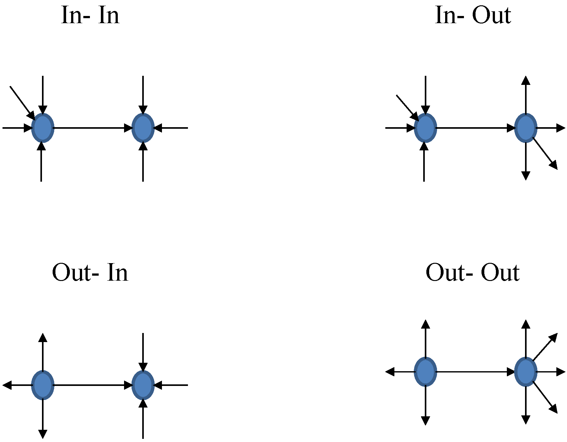
Figure 2.
Directed triangles and the corresponding (binary) clusterings associated with a node i. (a) Cycle clustering; (b) Middleman clustering; (c) In clustering; (d) Out clustering.Directed triangles and the corresponding clusterings.
Figure 2.
Directed triangles and the corresponding (binary) clusterings associated with a node i. (a) Cycle clustering; (b) Middleman clustering; (c) In clustering; (d) Out clustering.Directed triangles and the corresponding clusterings.

Figure 3.
The evolution of the size and the density of the electronic market for interbank deposits (e-MID) network. The left y-axis shows the number of active banks (in blue) and the right y-axis shows density (in green).
Figure 3.
The evolution of the size and the density of the electronic market for interbank deposits (e-MID) network. The left y-axis shows the number of active banks (in blue) and the right y-axis shows density (in green).
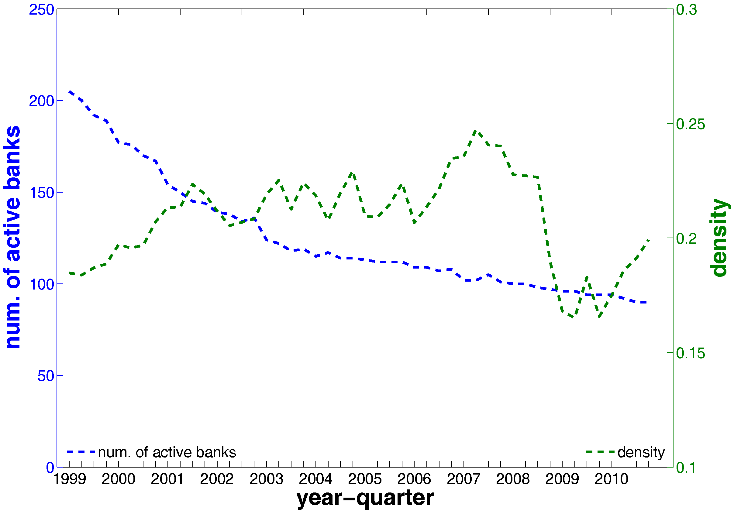
Figure 4.
The evolution of the basic statistics of weights in the undirected version () and in directed version ().
Figure 4.
The evolution of the basic statistics of weights in the undirected version () and in directed version ().

Figure 5.
Histograms of weights (i.e., in the undirected version and in the directed version) in two example quarters, Q1 and Q48. Note that for the sake of readability, we plot the number of the observations in log scale.
Figure 5.
Histograms of weights (i.e., in the undirected version and in the directed version) in two example quarters, Q1 and Q48. Note that for the sake of readability, we plot the number of the observations in log scale.

Figure 6.
The evolution of the basic statistics of degrees. Note that, by definition, the mean values of and are identical.
Figure 6.
The evolution of the basic statistics of degrees. Note that, by definition, the mean values of and are identical.
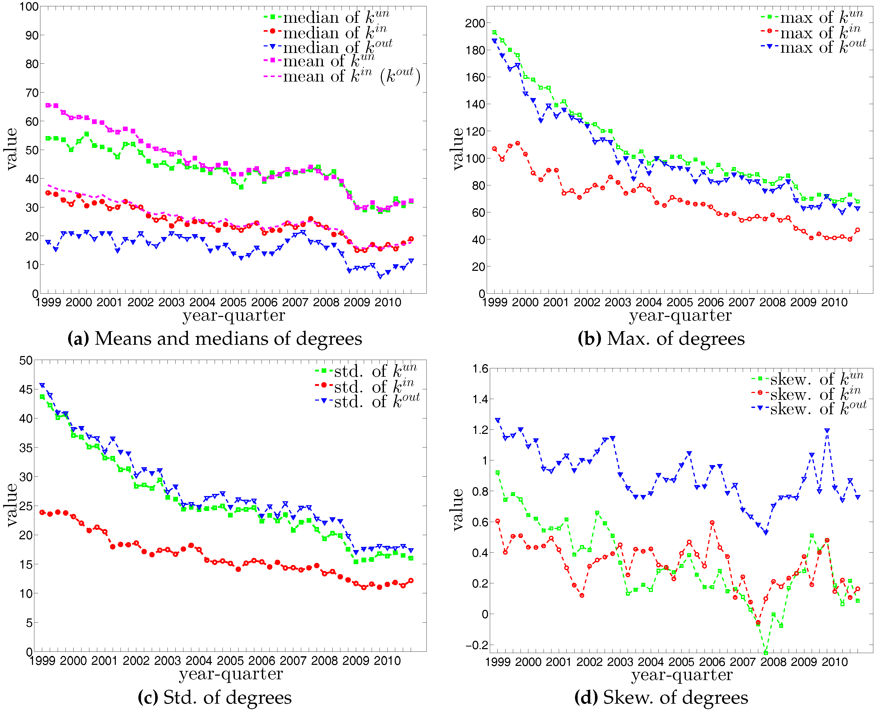
Figure 7.
Histograms of degrees in two example quarters, Q1 and Q48.

Figure 8.
The evolution of the basic statistics of strengths. Note that, by definition, the mean values of and are identical.
Figure 8.
The evolution of the basic statistics of strengths. Note that, by definition, the mean values of and are identical.
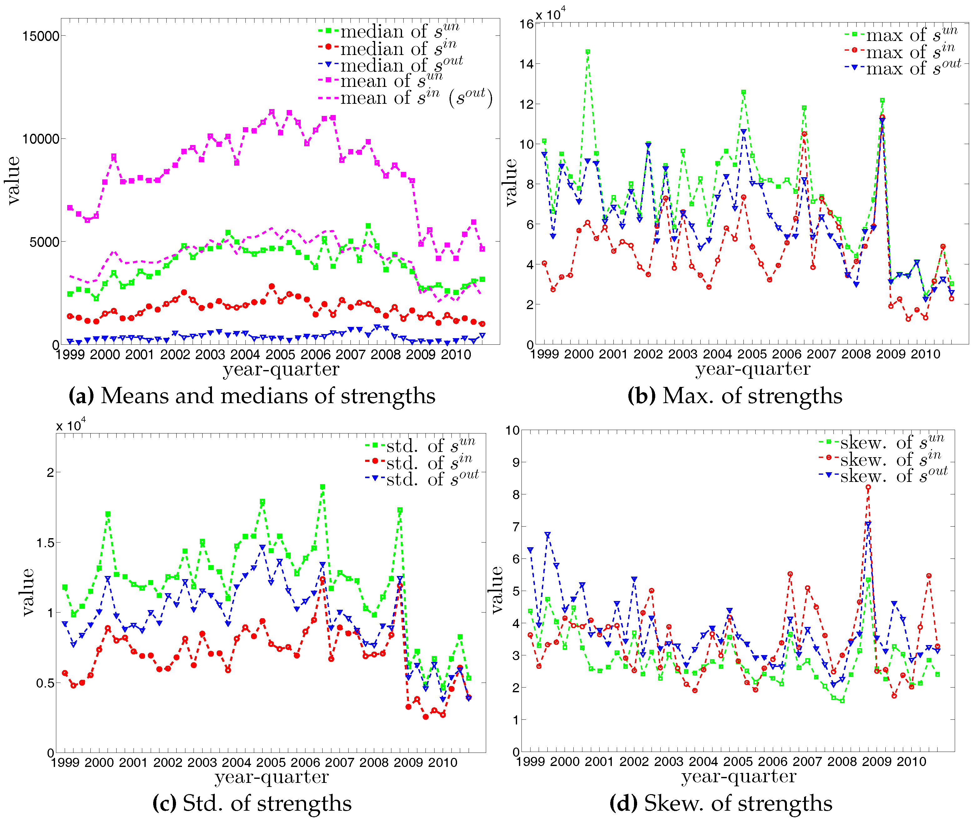
Figure 9.
Histograms of strengths in two example quarters, Q1 and Q48.
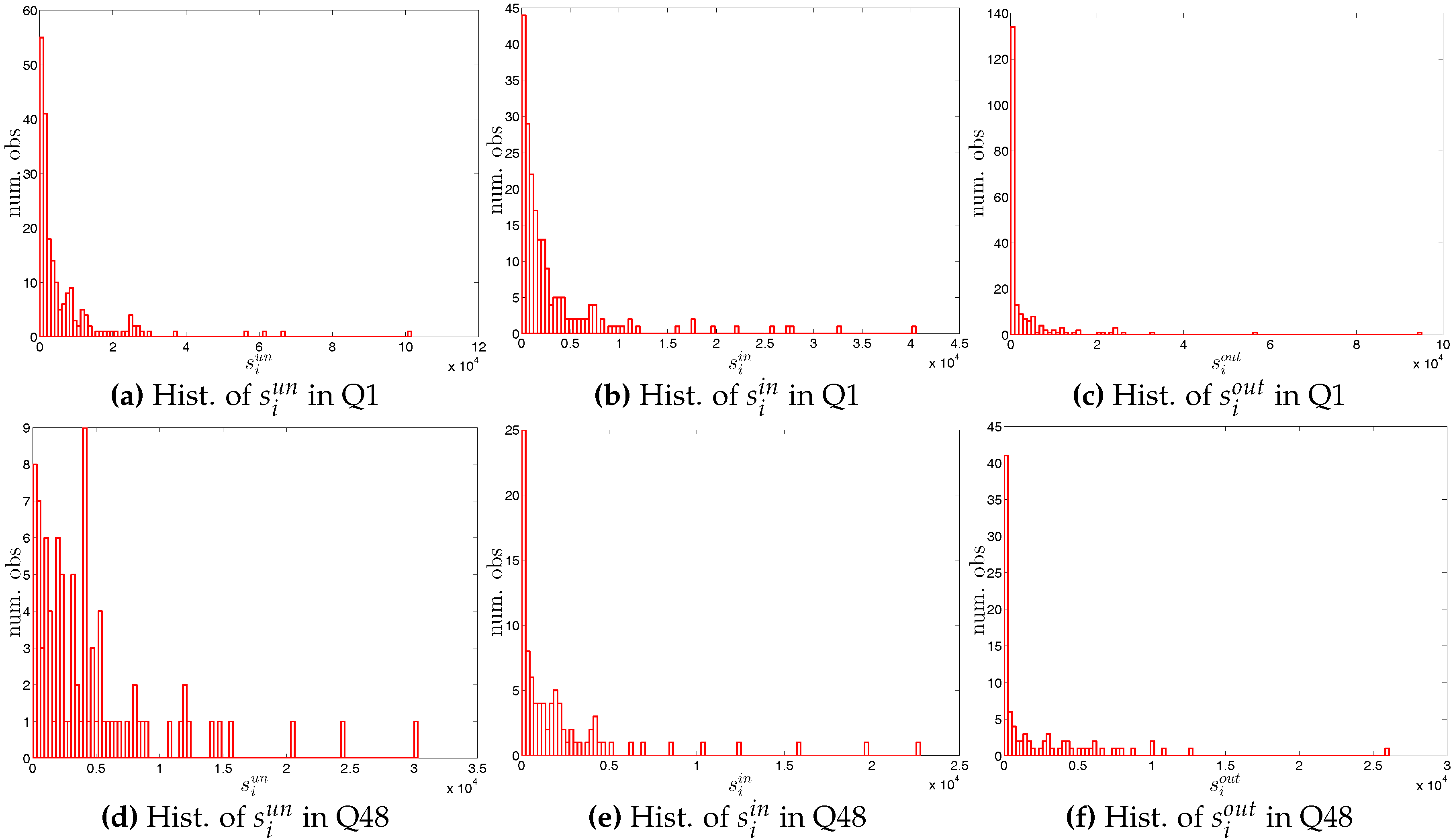
Figure 10.
The evolution of the Pearson correlation coefficients between degrees and strengths.

Figure 11.
Average degree of the nearest neighbors (ANND) (a,b), local assortativity (c,d), and local clustering coefficients (e,f) in the undirected binary e-MID network, in Q1 and Q48.Average degrees of nearest neighbors, local assortativity, and local clustering coefficients in the undirected binary e-MID network, in Q1 and Q48.

Figure 12.
Evolution of the overall assortativity indicator in the undirected binary e-MID network.
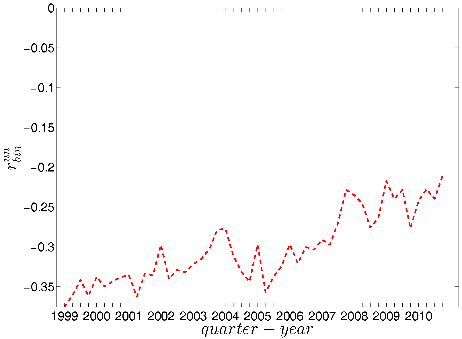
Figure 13.
Evolution of the average of local clustering coefficients (i.e., ) in the undirected binary e-MID network.
Figure 13.
Evolution of the average of local clustering coefficients (i.e., ) in the undirected binary e-MID network.
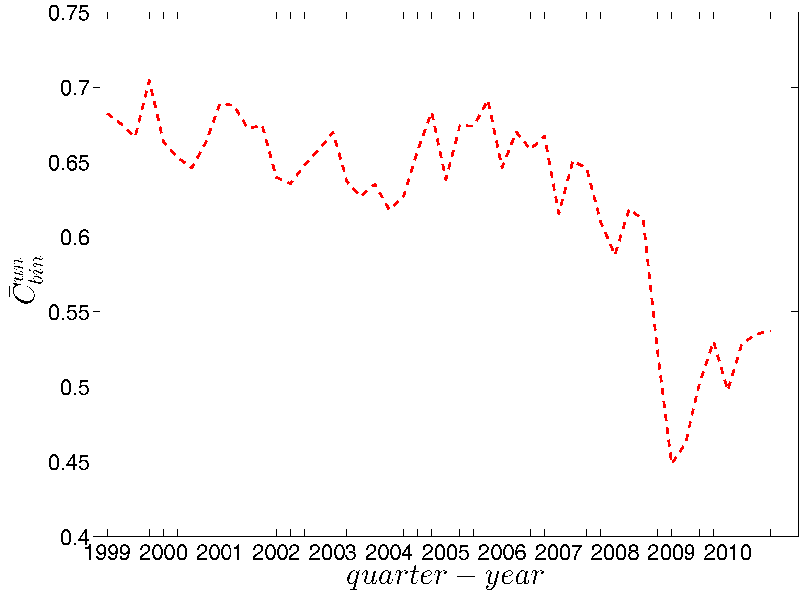
Figure 14.
ANND in the directed binary e-MID network, in Q1. (a) ; (b) ; (c) ; (d) .

Figure 15.
ANND in the directed binary e-MID network, in Q48. (a) ; (b) ; (c) ; (d) .

Figure 16.
Evolution of the overall assortativity indicators in the directed binary e-MID network.Evolution of the overall assortativity indicators in the directed binary e-MID network.
Figure 16.
Evolution of the overall assortativity indicators in the directed binary e-MID network.Evolution of the overall assortativity indicators in the directed binary e-MID network.

Figure 17.
Local assortativity in the directed binary e-MID network, in Q1. (a) ; (b) ; (c) ; (d) .
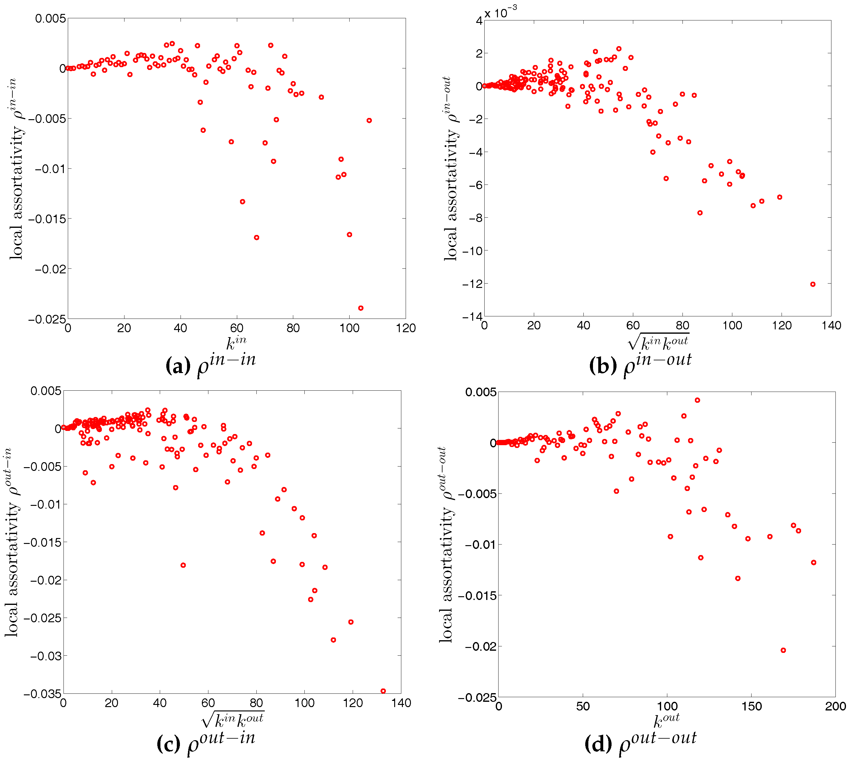
Figure 18.
Local assortativity in the directed binary e-MID network, in Q48. (a) ; (b) ; (c) ; (d) .
Figure 18.
Local assortativity in the directed binary e-MID network, in Q48. (a) ; (b) ; (c) ; (d) .
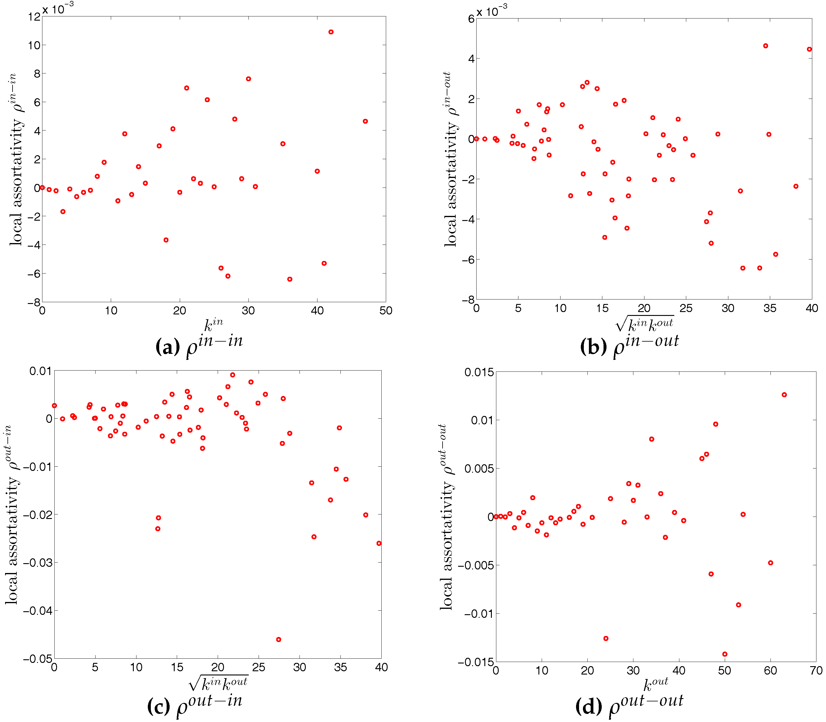
Figure 19.
Local clustering coefficients (a) ; (b) ; (c) ; (d) in the directed binary e-MID network, in Q1.
Figure 19.
Local clustering coefficients (a) ; (b) ; (c) ; (d) in the directed binary e-MID network, in Q1.
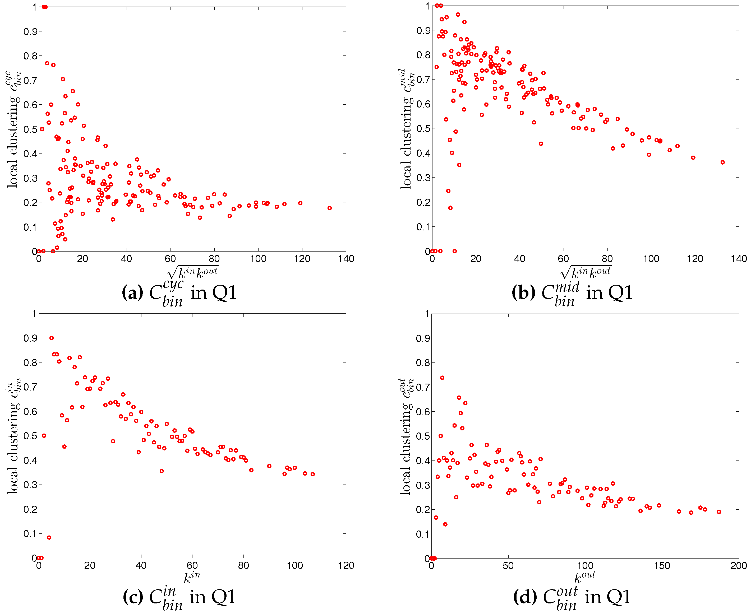
Figure 20.
Local clustering coefficients (a) ; (b) ; (c) ; (d) in the directed binary e-MID network, in Q48.
Figure 20.
Local clustering coefficients (a) ; (b) ; (c) ; (d) in the directed binary e-MID network, in Q48.


Figure 21.
Evolution of the averages of local clustering coefficients (i.e., , , , and ) in the directed binary e-MID network.
Figure 21.
Evolution of the averages of local clustering coefficients (i.e., , , , and ) in the directed binary e-MID network.

Figure 22.
(a,b) ANND; (c,d) local assortativity ; (e,f) local clustering coefficients in the observed e-MID network and in the UBCM, in Q1 and Q48.
Figure 22.
(a,b) ANND; (c,d) local assortativity ; (e,f) local clustering coefficients in the observed e-MID network and in the UBCM, in Q1 and Q48.

Figure 23.
Evolution of (a) ; (b) ; and (c) in the observed e-MID network and in the undirected binary configuration model (UBCM).
Figure 23.
Evolution of (a) ; (b) ; and (c) in the observed e-MID network and in the undirected binary configuration model (UBCM).
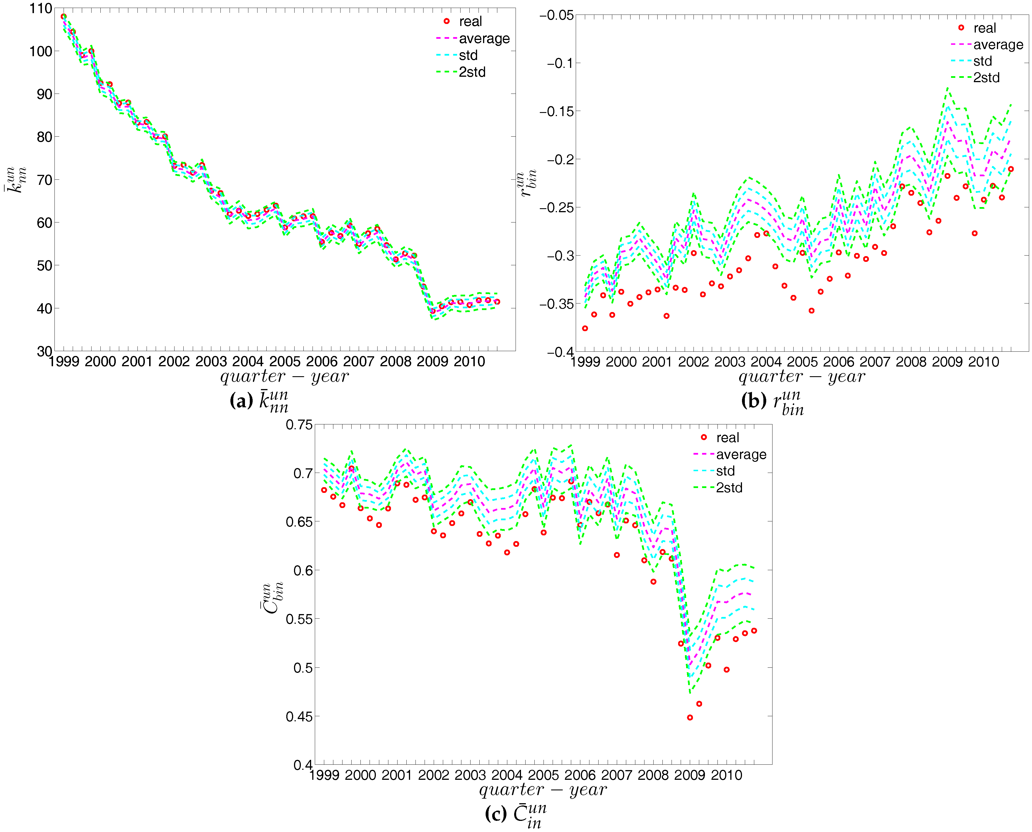
Figure 24.
ANND in the observed e-MID network and in the DBCM, in Q1. (a) ; (b) ; (c) ; (d) .

Figure 25.
ANND in the observed e-MID network and in the DBCM, in Q48. (a) ; (b) ; (c) ; (d) .

Figure 26.
Local assortativity in the observed e-MID network and in the DBCM, in Q1. (a) ; (b) ; (c) ; (d) .
Figure 26.
Local assortativity in the observed e-MID network and in the DBCM, in Q1. (a) ; (b) ; (c) ; (d) .
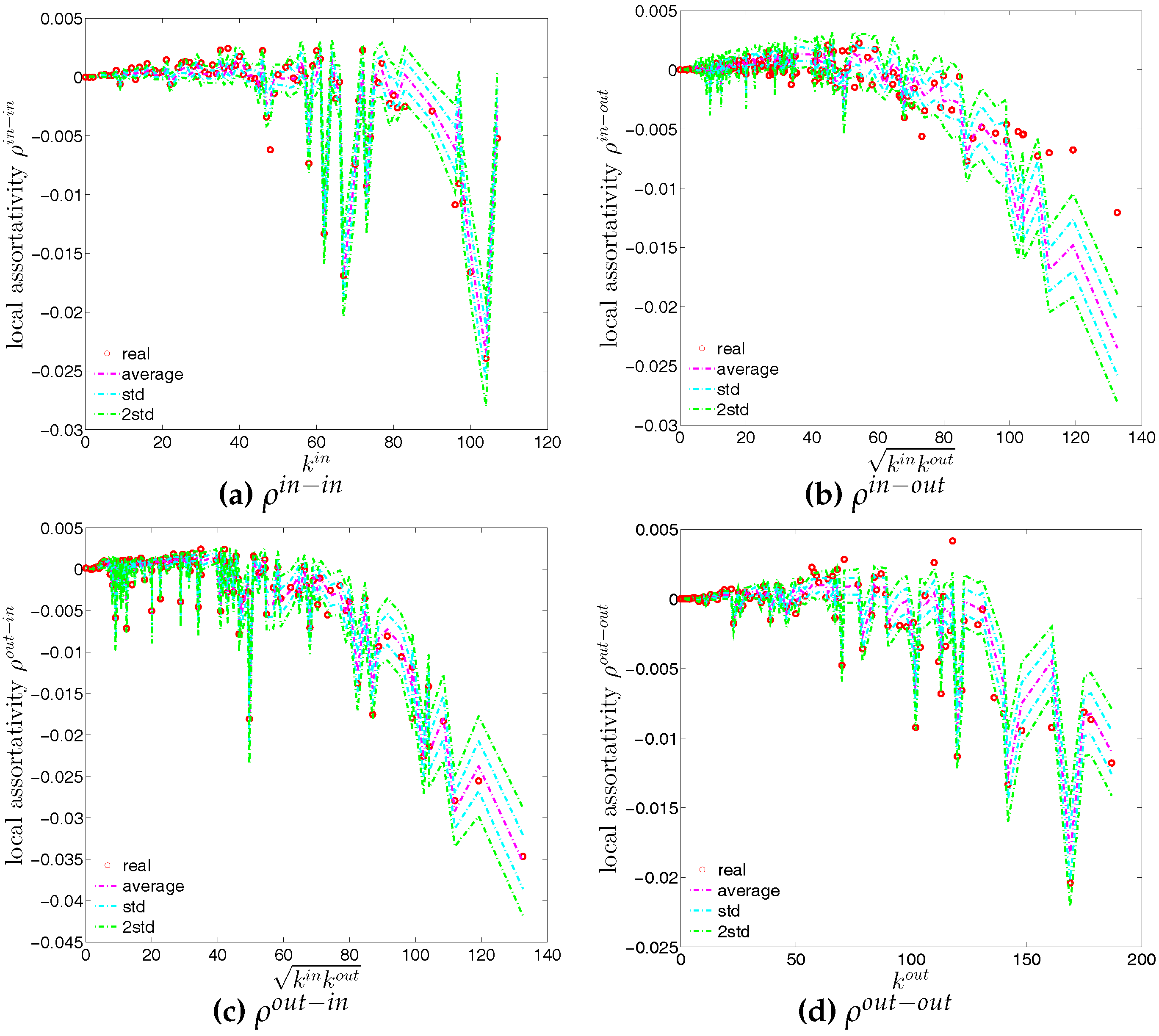
Figure 27.
Local assortativity in the observed e-MID network and in the DBCM, in Q48. (a) ; (b) ; (c) ; (d) .
Figure 27.
Local assortativity in the observed e-MID network and in the DBCM, in Q48. (a) ; (b) ; (c) ; (d) .
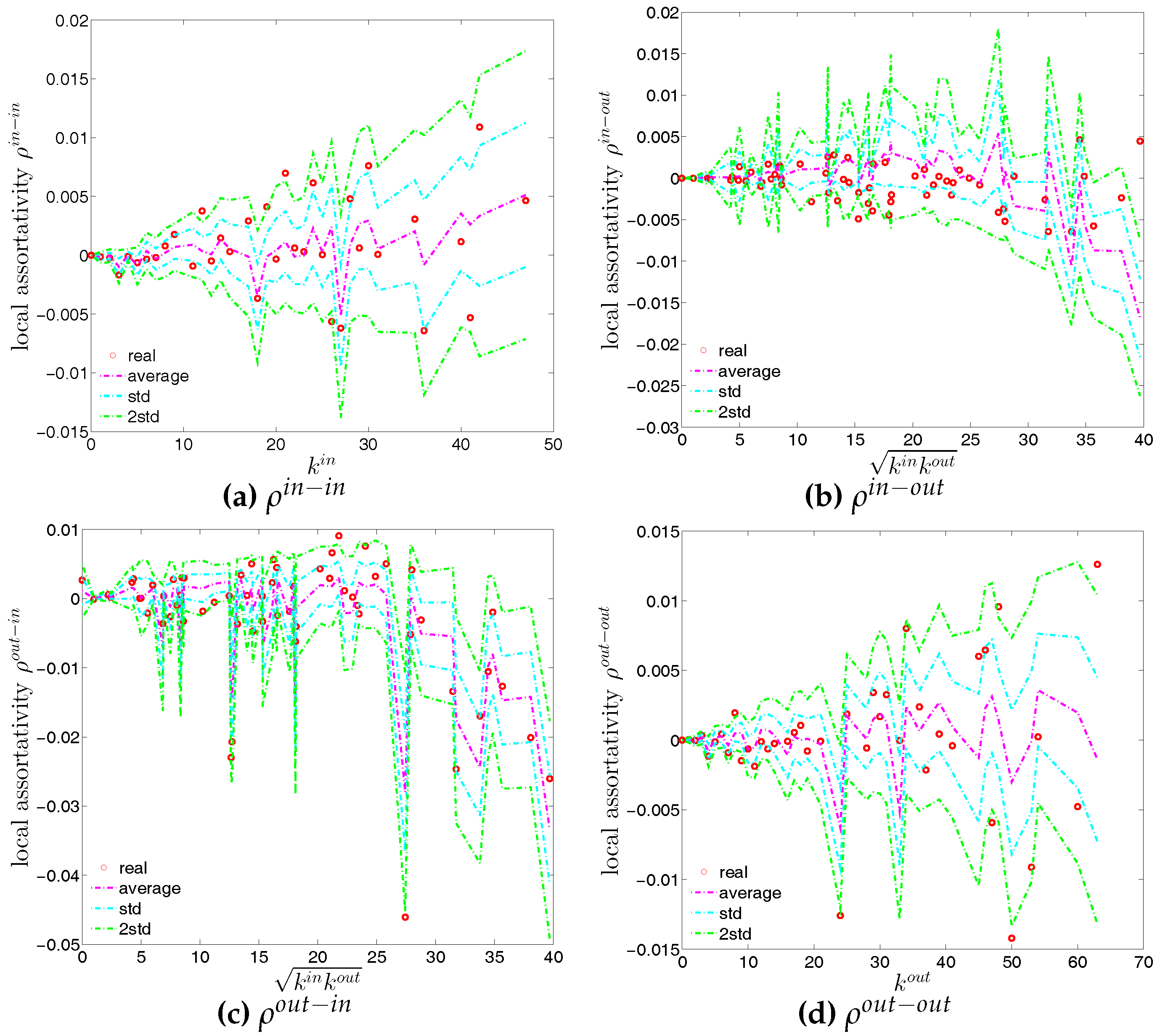
Figure 28.
Local clustering coefficients (a) ; (b) ; (c) ; (d) in the observed e-MID network and in DBCM, in Q1.
Figure 28.
Local clustering coefficients (a) ; (b) ; (c) ; (d) in the observed e-MID network and in DBCM, in Q1.

Figure 29.
Local clustering coefficients (a) ; (b) ; (c) ; (d) in the observed e-MID network and in DBCM, in Q48.
Figure 29.
Local clustering coefficients (a) ; (b) ; (c) ; (d) in the observed e-MID network and in DBCM, in Q48.

Figure 30.
Evolution of the averages of ANNDs in the observed e-MID network and in the DBCM. (a) ; (b) ; (c) ; (d) .
Figure 30.
Evolution of the averages of ANNDs in the observed e-MID network and in the DBCM. (a) ; (b) ; (c) ; (d) .
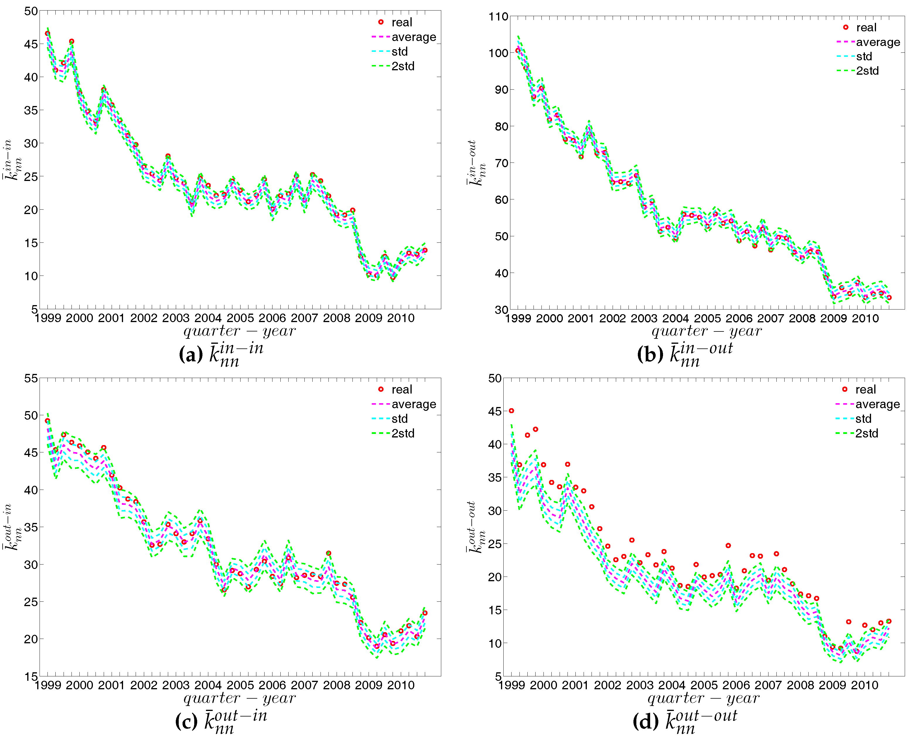
Figure 31.
Evolution of the global assortativity indicators in the observed e-MID network and in the DBCM. (a) ; (b) ; (c) ; (d) .
Figure 31.
Evolution of the global assortativity indicators in the observed e-MID network and in the DBCM. (a) ; (b) ; (c) ; (d) .

Figure 32.
Evolution of the averages of clustering coefficients in the observed e-MID network and in the DBCM. (a) ; (b) ; (c) ; (d) .
Figure 32.
Evolution of the averages of clustering coefficients in the observed e-MID network and in the DBCM. (a) ; (b) ; (c) ; (d) .
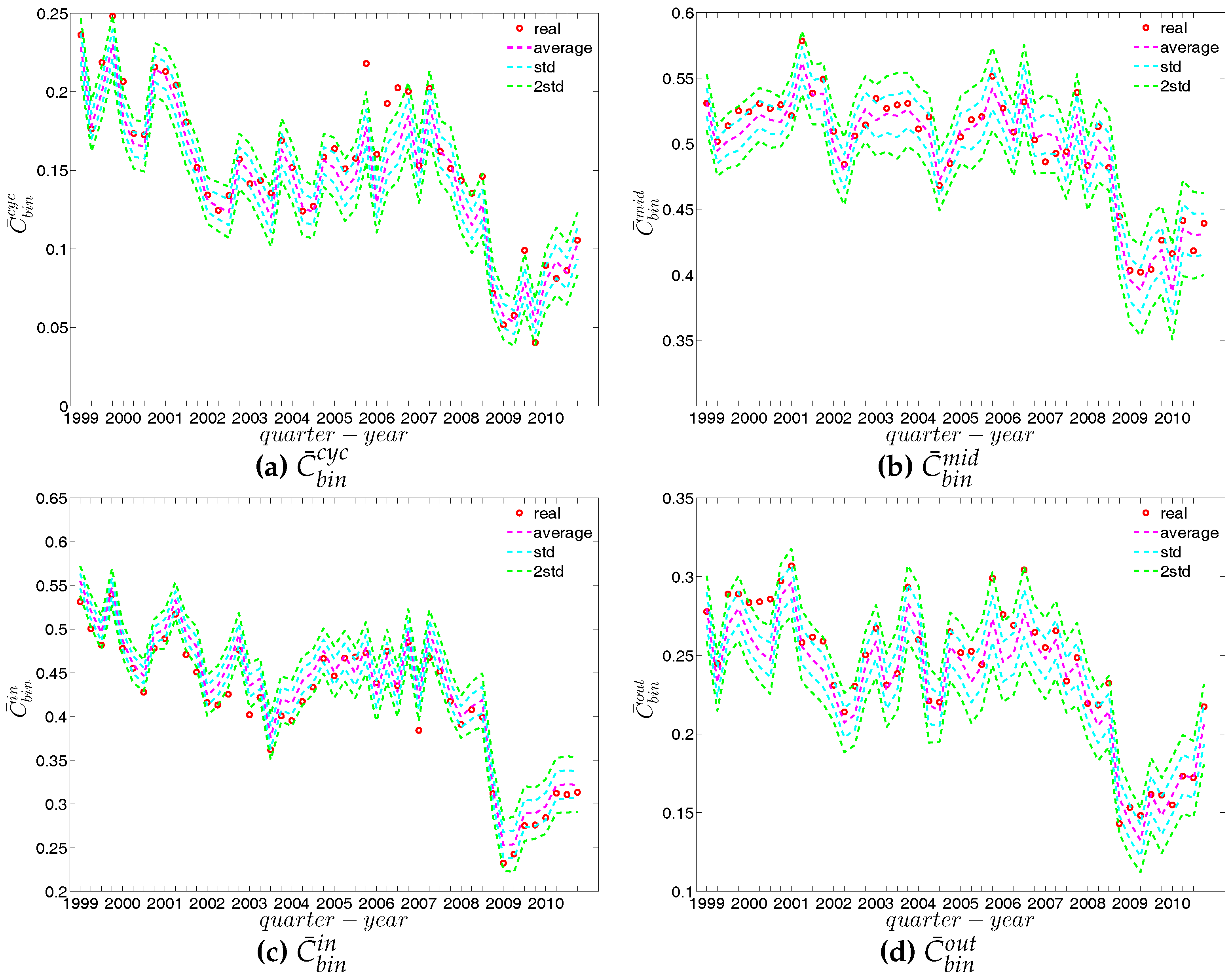
Figure 33.
Average strength of the nearest neighbors (ANNS) in the undirected weighted e-MID network, in Q1 and Q48.
Figure 33.
Average strength of the nearest neighbors (ANNS) in the undirected weighted e-MID network, in Q1 and Q48.

Figure 34.
Evolution of global weighted assortativity in the undirected weighted e-MID network.

Figure 35.
Local clustering coefficients in the undirected weighted e-MID network, in Q1 and Q48.

Figure 36.
Evolution of the average of local weighted clustering coefficients (i.e., ) in the undirected weighted e-MID network.
Figure 36.
Evolution of the average of local weighted clustering coefficients (i.e., ) in the undirected weighted e-MID network.
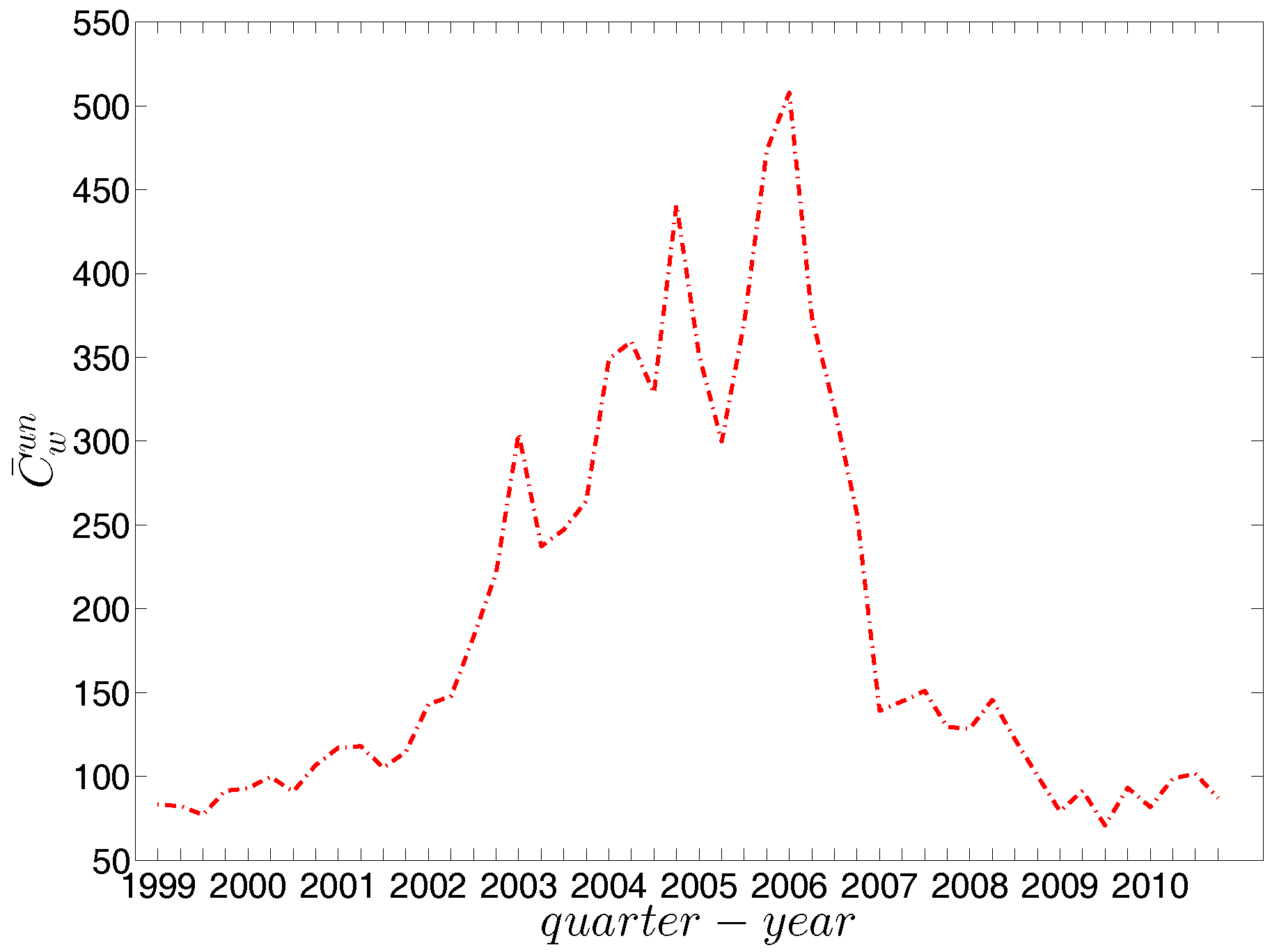
Figure 37.
ANNSs in the directed weighted e-MID network, in Q1. (a) ; (b) ; (c) ; (d) .

Figure 38.
ANNSs in the directed weighted e-MID network, in Q48. (a) ; (b) ; (c) ; (d) .

Figure 39.
Evolution of the directed weighted assortativity indicators, i.e., , , , and in the directed weighted e-MID network.
Figure 39.
Evolution of the directed weighted assortativity indicators, i.e., , , , and in the directed weighted e-MID network.
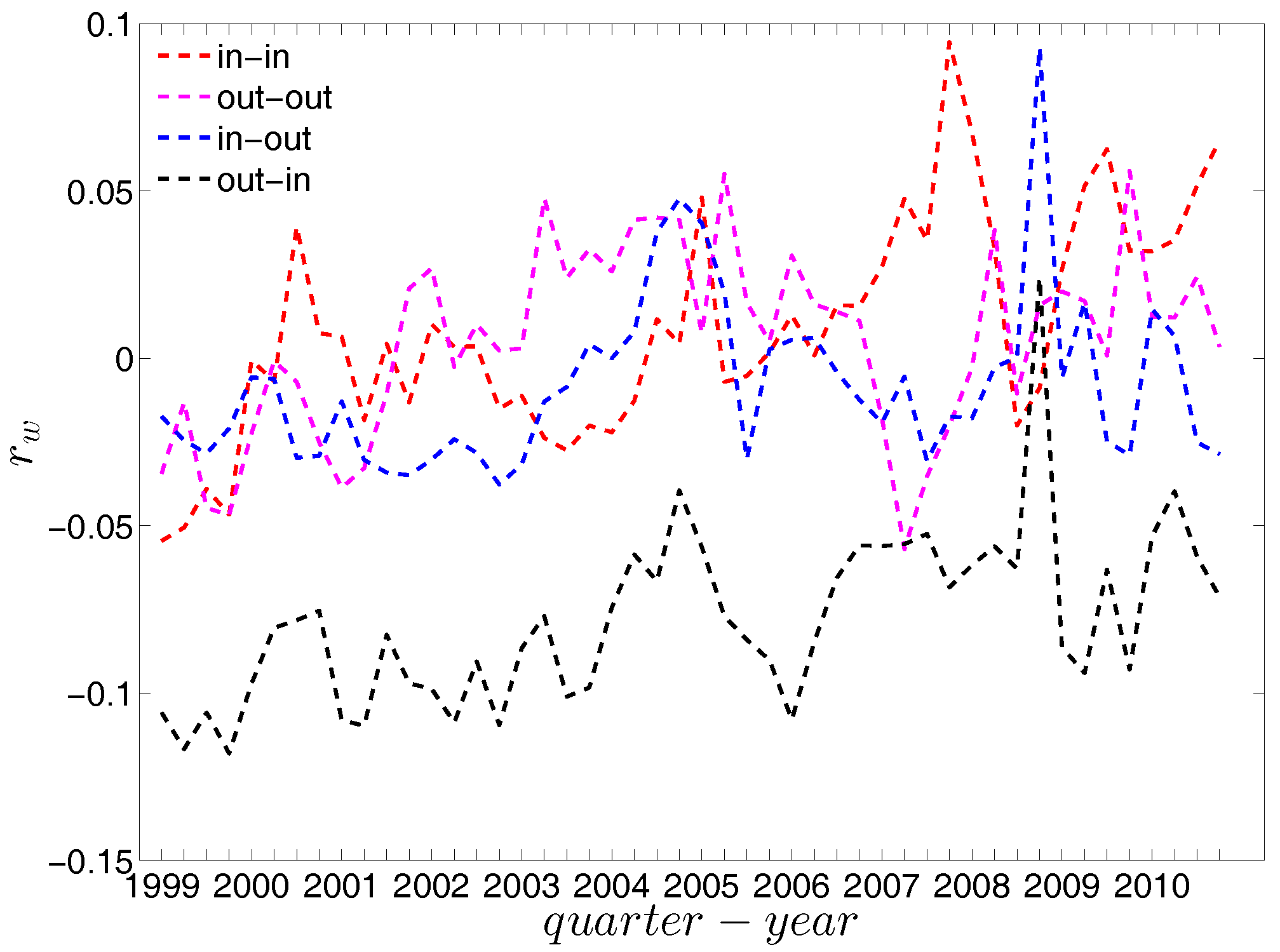
Figure 40.
Local weighted clustering coefficients in the directed weighted e-MID network, in Q1. (a) ; (b) ; (c) ; (d) .
Figure 40.
Local weighted clustering coefficients in the directed weighted e-MID network, in Q1. (a) ; (b) ; (c) ; (d) .

Figure 41.
Local weighted clustering coefficients in the directed weighted e-MID network, in Q48. (a) ; (b) ; (c) ; (d) .
Figure 41.
Local weighted clustering coefficients in the directed weighted e-MID network, in Q48. (a) ; (b) ; (c) ; (d) .
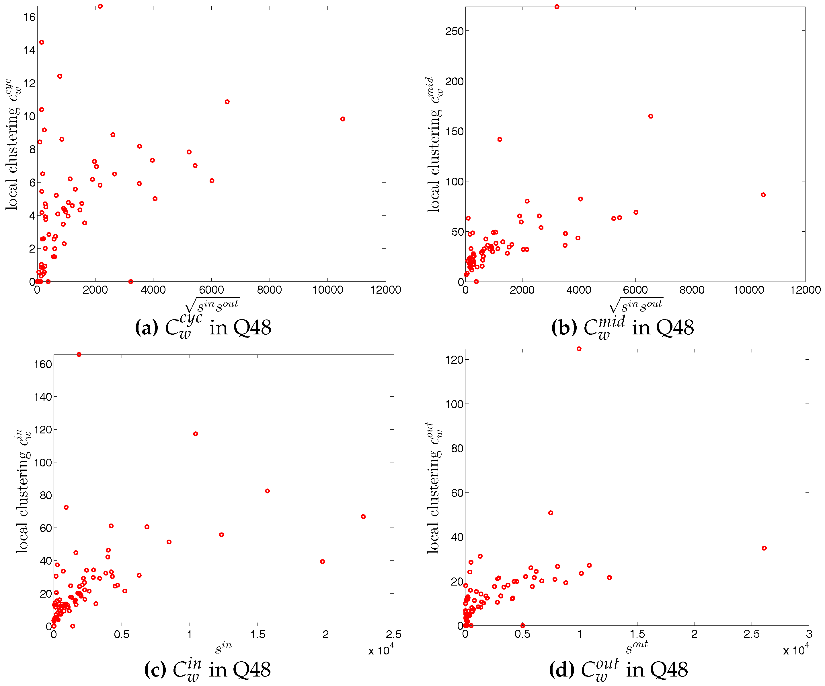
Figure 42.
Evolution of the averages of local weighted clustering coefficients, i.e., , , , and in the directed weighted e-MID network.
Figure 42.
Evolution of the averages of local weighted clustering coefficients, i.e., , , , and in the directed weighted e-MID network.
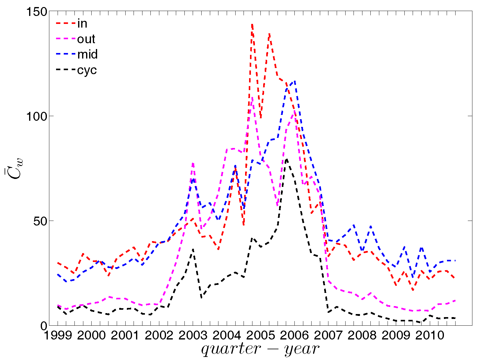
Figure 43.
ANNS in the observed e-MID network and in the UWCM, in Q1 and Q48.

Figure 44.
Local weighted clustering coefficients in the observed e-MID network and in the UWCM, in Q1 and Q48.
Figure 44.
Local weighted clustering coefficients in the observed e-MID network and in the UWCM, in Q1 and Q48.
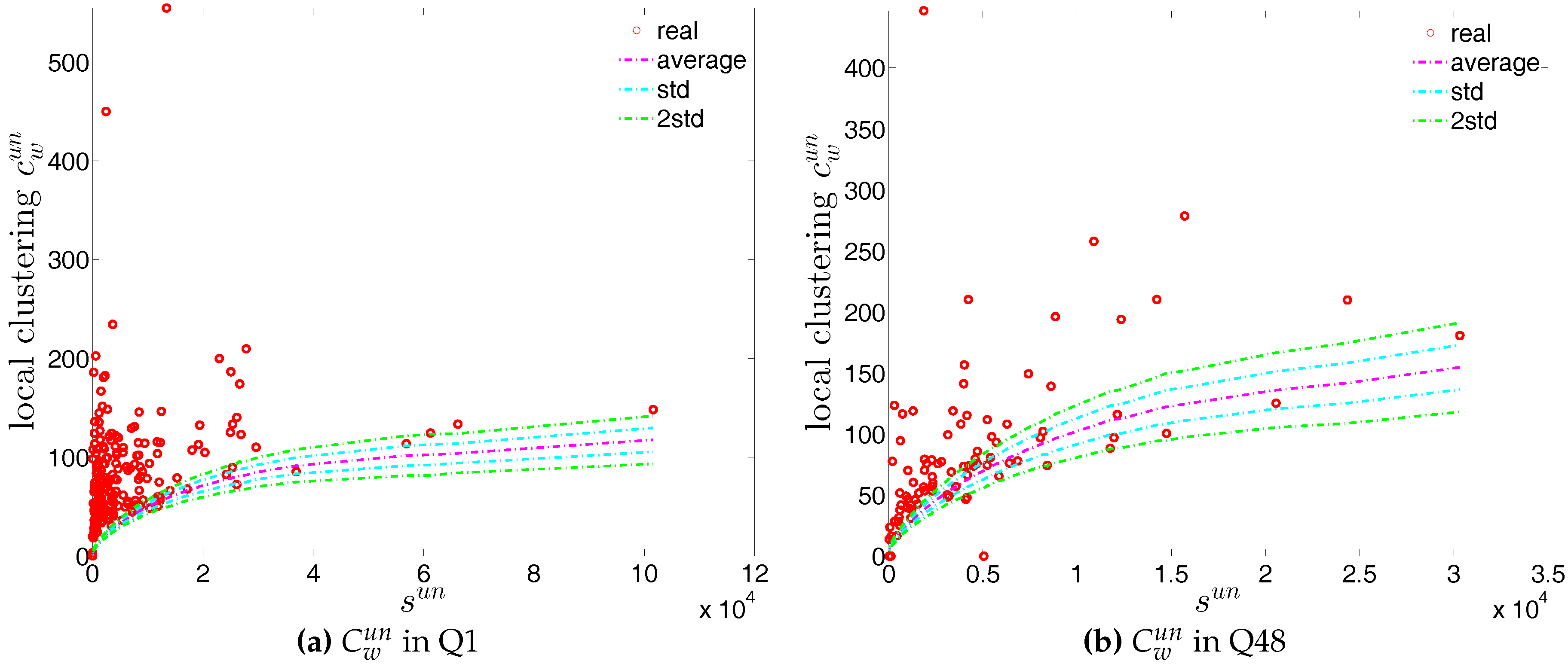
Figure 45.
ANNS in the observed e-MID network and in the UECM, in Q1 and Q48.

Figure 46.
Local weighted clustering coefficients in the observed e-MID network and in the UECM, in Q1 and Q48.
Figure 46.
Local weighted clustering coefficients in the observed e-MID network and in the UECM, in Q1 and Q48.

Figure 47.
z-scores of vs. in the UWCM and the UECM, in Q1 and in Q48. Panel (a) for z-scores of in Q1; panel (b) for z-scores of in Q48.
Figure 47.
z-scores of vs. in the UWCM and the UECM, in Q1 and in Q48. Panel (a) for z-scores of in Q1; panel (b) for z-scores of in Q48.
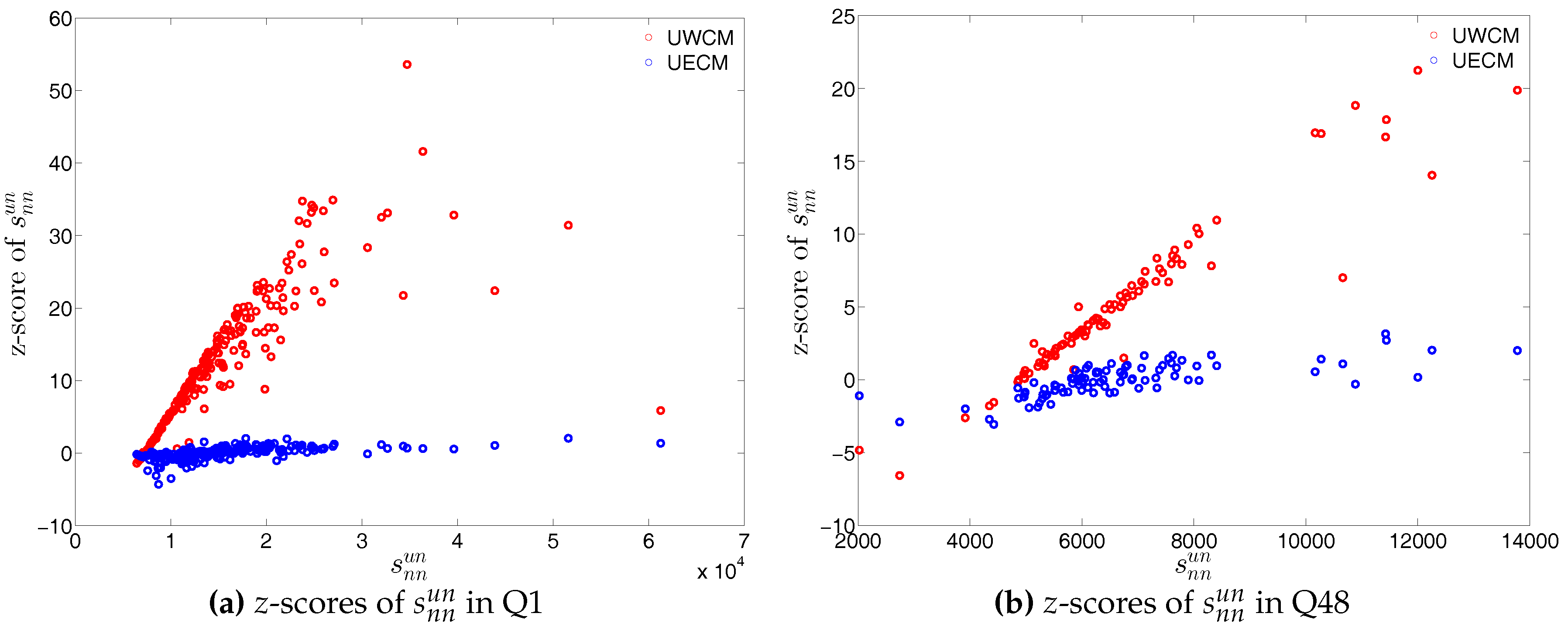
Figure 48.
z-scores of vs. in the UWCM and the UECM. (a) for z-scores of in Q1; (b) for z-scores of in Q48.
Figure 48.
z-scores of vs. in the UWCM and the UECM. (a) for z-scores of in Q1; (b) for z-scores of in Q48.

Figure 49.
Evolution of (a) ; (b) ; and (c) in the observed e-MID network and in the UWCM.
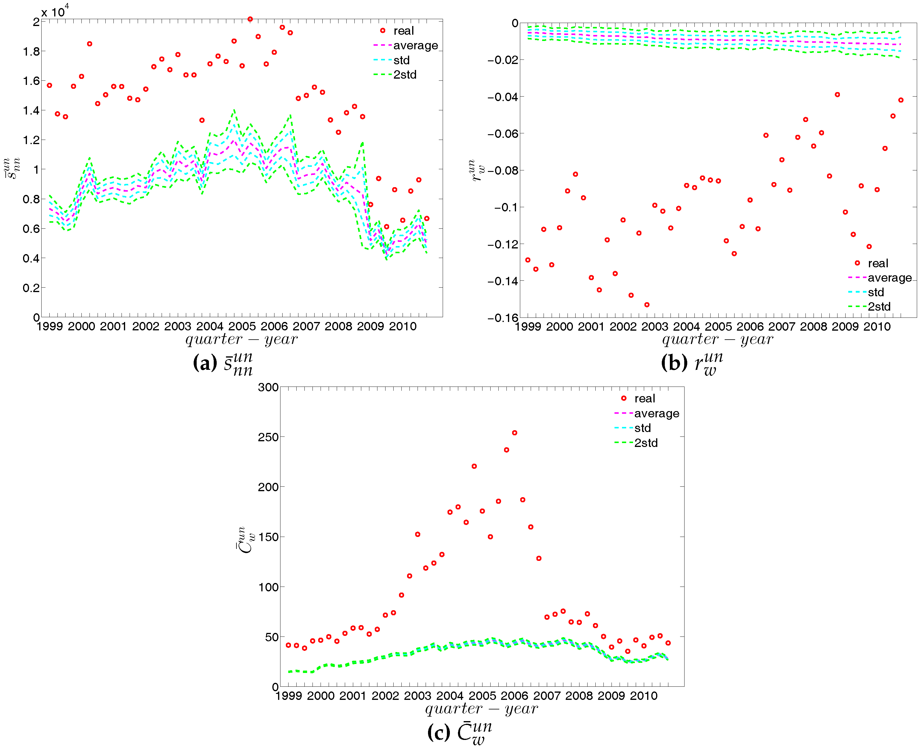
Figure 50.
Evolution of (a) ; (b) ; and (c) in the observed e-MID network and in the UECM.

Figure 51.
ANNSs in the observed e-MID network and in the DWCM, in Q1. (a) ; (b) ; (c) ; (d) .

Figure 52.
ANNSs in the observed e-MID network and in the DWCM, in Q48. (a) ; (b) ; (c) ; (d) .
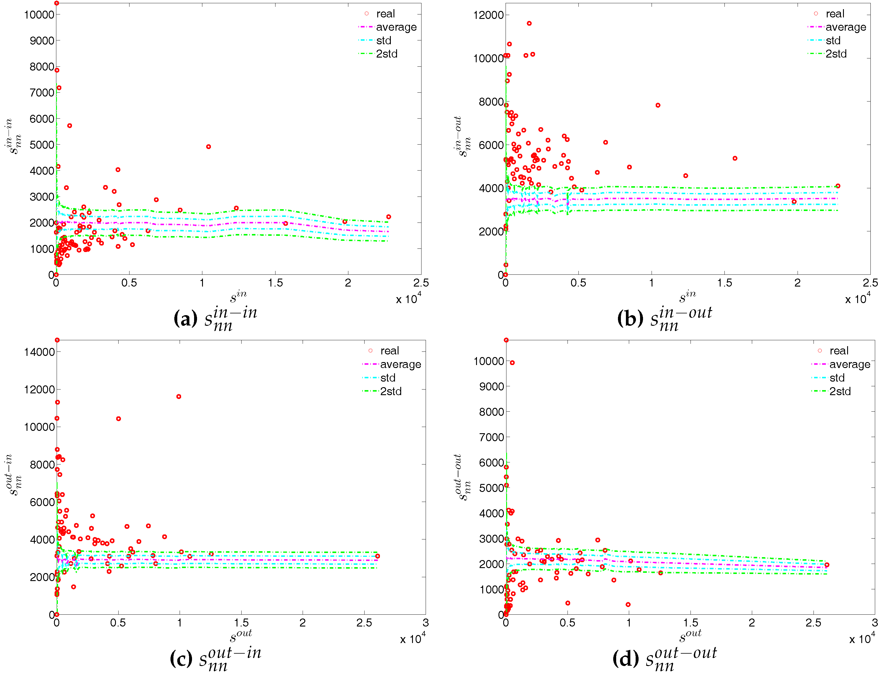
Figure 53.
ANNSs in the observed e-MID network and in the DECM, in Q1. (a) ; (b) ; (c) ; (d) .

Figure 54.
ANNSs in the observed e-MID network and in the DECM, in Q48. (a) ; (b) ; (c) ; (d) .
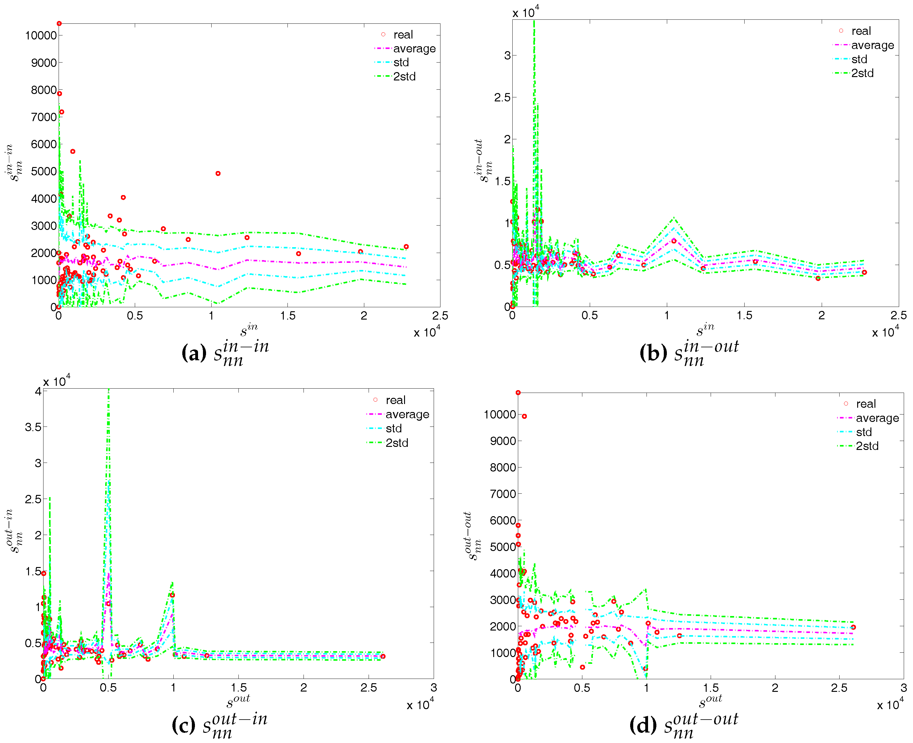
Figure 55.
z-scores of ANNSs vs. ANNSs, in the DWCM and DECM models, in Q1. (a) for ; (b) for ; (c) for ; (d) for .
Figure 55.
z-scores of ANNSs vs. ANNSs, in the DWCM and DECM models, in Q1. (a) for ; (b) for ; (c) for ; (d) for .
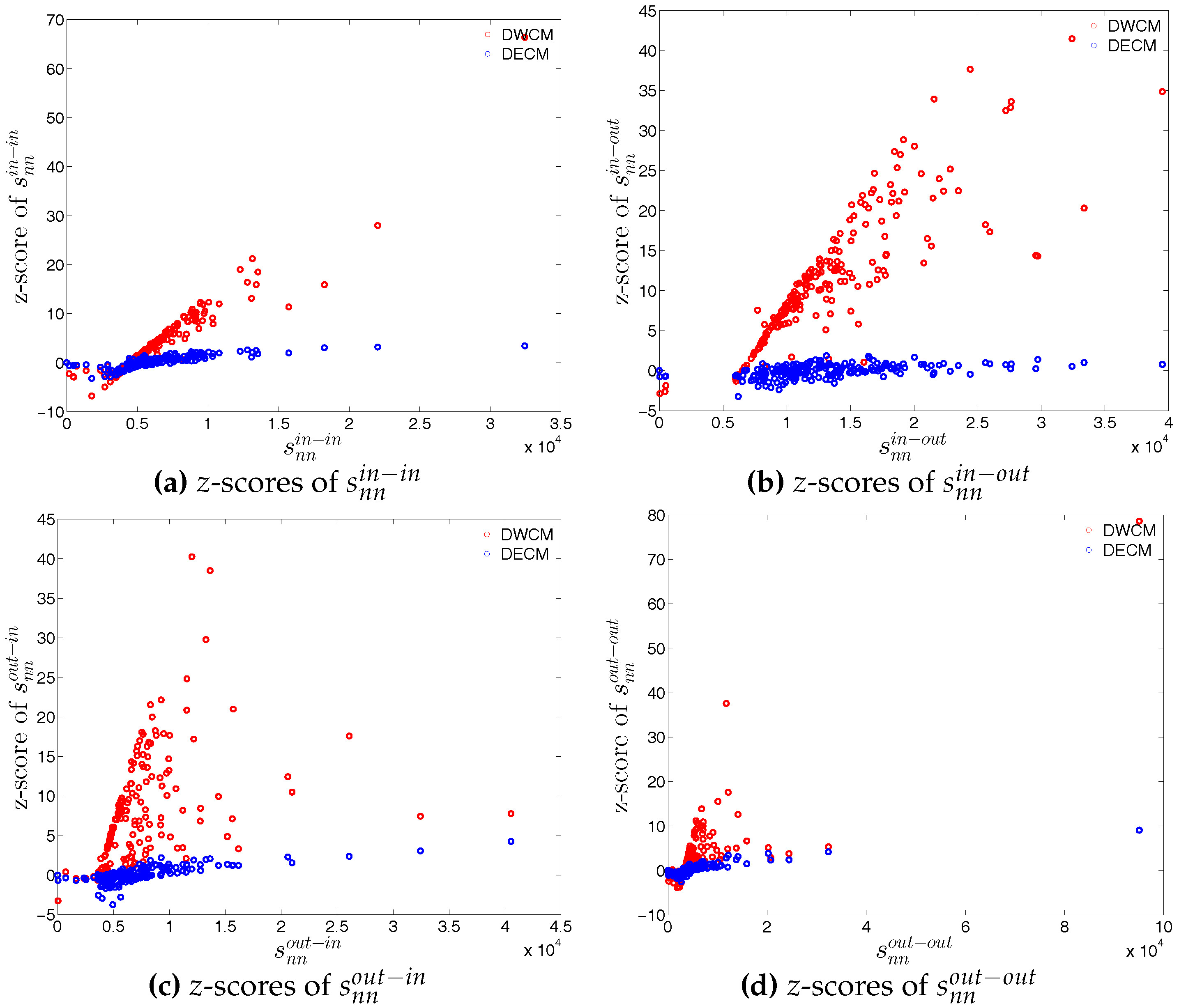
Figure 56.
z-scores of ANNSs vs. ANNSs, in the DWCM and DECM models, in Q48. (a) for ; (b) for ; (c) for ; (d) for .
Figure 56.
z-scores of ANNSs vs. ANNSs, in the DWCM and DECM models, in Q48. (a) for ; (b) for ; (c) for ; (d) for .

Figure 57.
Local weighted clustering coefficients in the observed e-MID network and in the DWCM, in Q1. (a) ; (b) ; (c) ; (d) .
Figure 57.
Local weighted clustering coefficients in the observed e-MID network and in the DWCM, in Q1. (a) ; (b) ; (c) ; (d) .
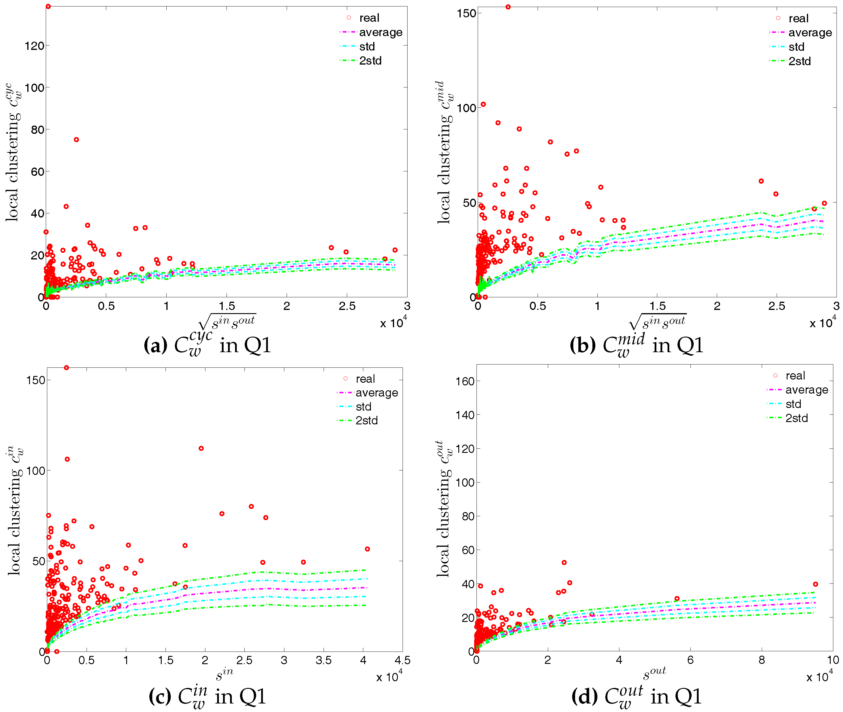
Figure 58.
Local weighted clustering coefficients in the observed e-MID network and in the DWCM, in Q48. (a) ; (b) ; (c) ; (d) .
Figure 58.
Local weighted clustering coefficients in the observed e-MID network and in the DWCM, in Q48. (a) ; (b) ; (c) ; (d) .

Figure 59.
Local weighted clustering coefficients in the observed e-MID network and in the DECM, in Q1. (a) ; (b) ; (c) ; (d) .
Figure 59.
Local weighted clustering coefficients in the observed e-MID network and in the DECM, in Q1. (a) ; (b) ; (c) ; (d) .

Figure 60.
Local weighted clustering coefficients in the observed e-MID network and in the DECM, in Q48. (a) ; (b) ; (c) ; (d) .
Figure 60.
Local weighted clustering coefficients in the observed e-MID network and in the DECM, in Q48. (a) ; (b) ; (c) ; (d) .

Figure 61.
z-scores of vs. , evaluated under the DWCM and DECM models, in Q1. (a) for ; (b) for ; (c) for ; (d) for .
Figure 61.
z-scores of vs. , evaluated under the DWCM and DECM models, in Q1. (a) for ; (b) for ; (c) for ; (d) for .

Figure 62.
z-scores of vs. , evaluated under the DWCM and DECM models, in Q48. (a) for ; (b) for ; (c) for ; (d) for .
Figure 62.
z-scores of vs. , evaluated under the DWCM and DECM models, in Q48. (a) for ; (b) for ; (c) for ; (d) for .
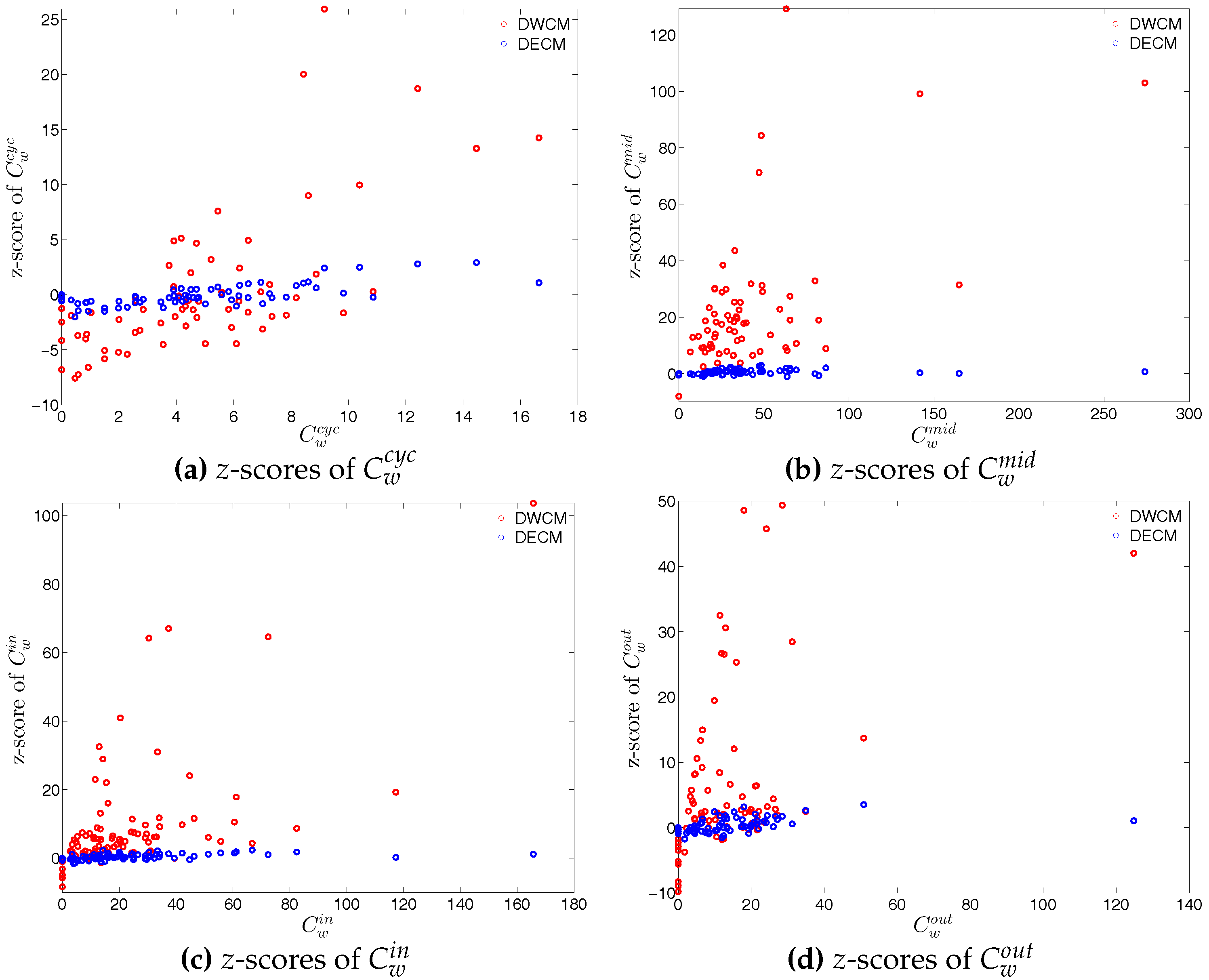
Figure 63.
Evolution of the averages of ANNSs in the observed e-MID network and in the DWCM. (a) ; (b) ; (c) ; (d) .
Figure 63.
Evolution of the averages of ANNSs in the observed e-MID network and in the DWCM. (a) ; (b) ; (c) ; (d) .
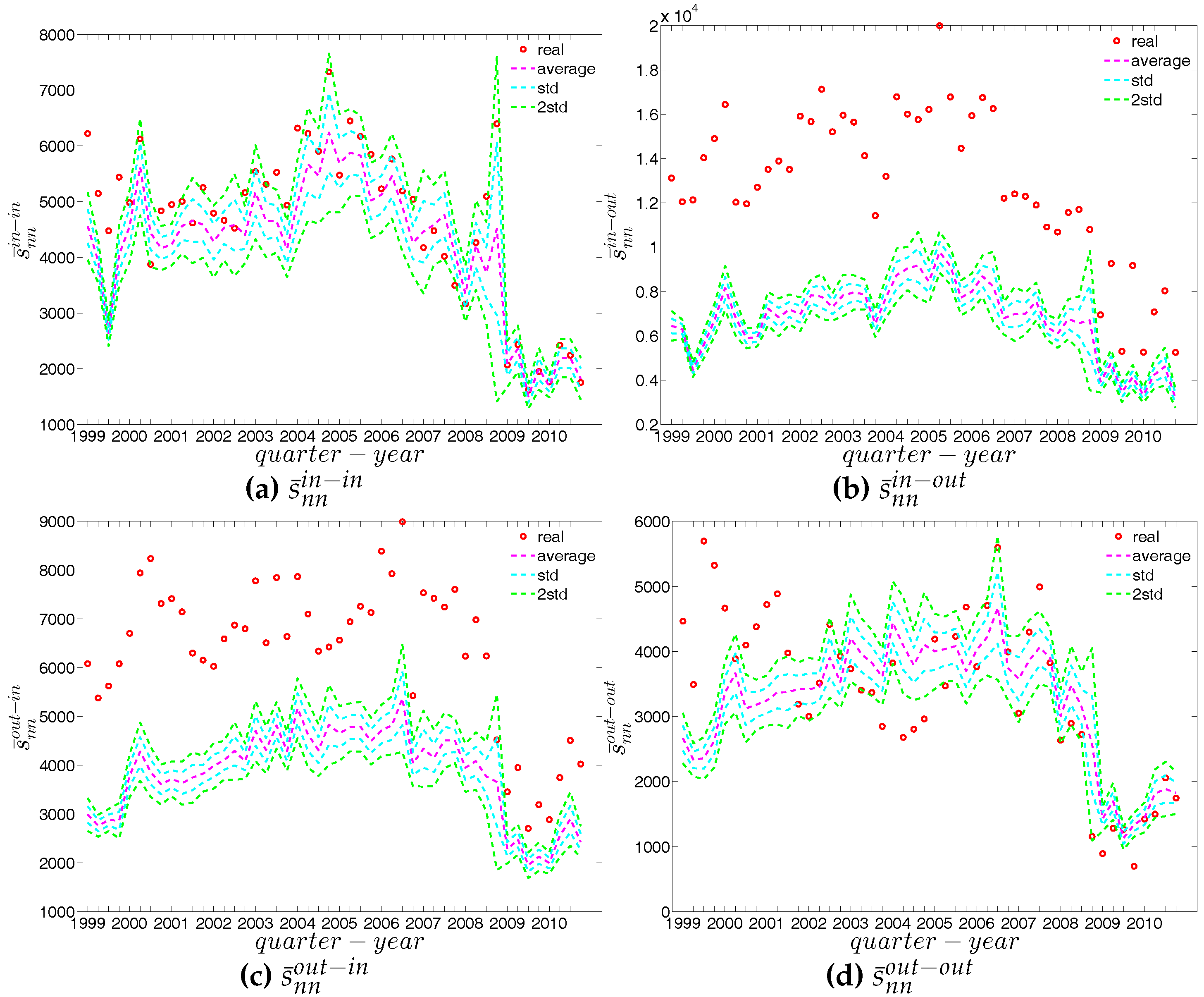
Figure 64.
Evolution of the global weighted assortativity indicators in the observed e-MID network and in the DWCM. (a) ; (b) ; (c) ; (d) .
Figure 64.
Evolution of the global weighted assortativity indicators in the observed e-MID network and in the DWCM. (a) ; (b) ; (c) ; (d) .

Figure 65.
Evolution of the averages of local weighted clustering coefficients in the observed e-MID network and in the DWCM. (a) ; (b) ; (c) ; (d) .
Figure 65.
Evolution of the averages of local weighted clustering coefficients in the observed e-MID network and in the DWCM. (a) ; (b) ; (c) ; (d) .
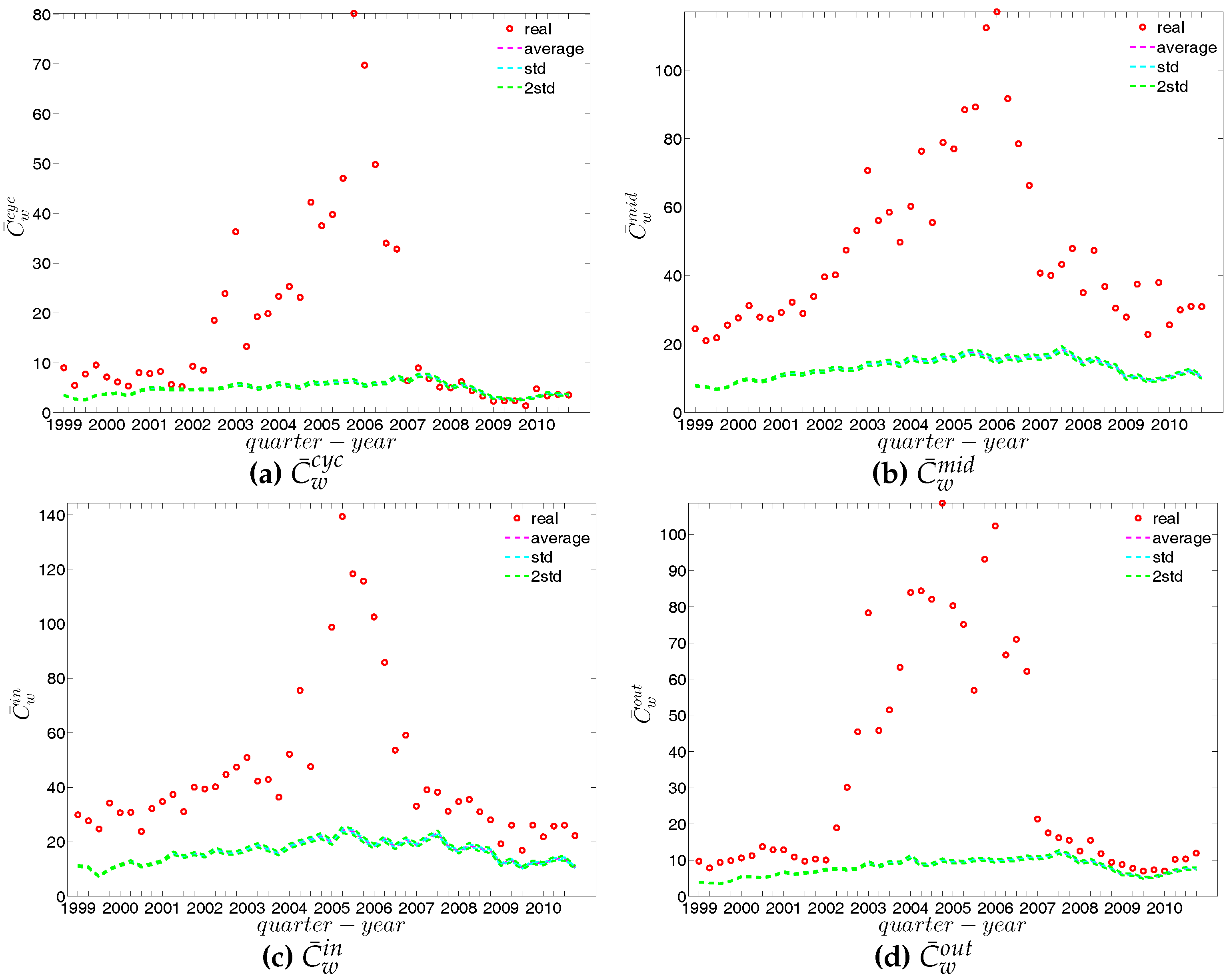
Figure 66.
Evolution of the averages of ANNSs in the observed e-MID network and in the DECM. (a) ; (b) ; (c) ; (d) .
Figure 66.
Evolution of the averages of ANNSs in the observed e-MID network and in the DECM. (a) ; (b) ; (c) ; (d) .

Figure 67.
Evolution of the global weighted assortativity indicators in the observed e-MID network and in the DECM. (a) ; (b) (b); (c) ; (d) .
Figure 67.
Evolution of the global weighted assortativity indicators in the observed e-MID network and in the DECM. (a) ; (b) (b); (c) ; (d) .
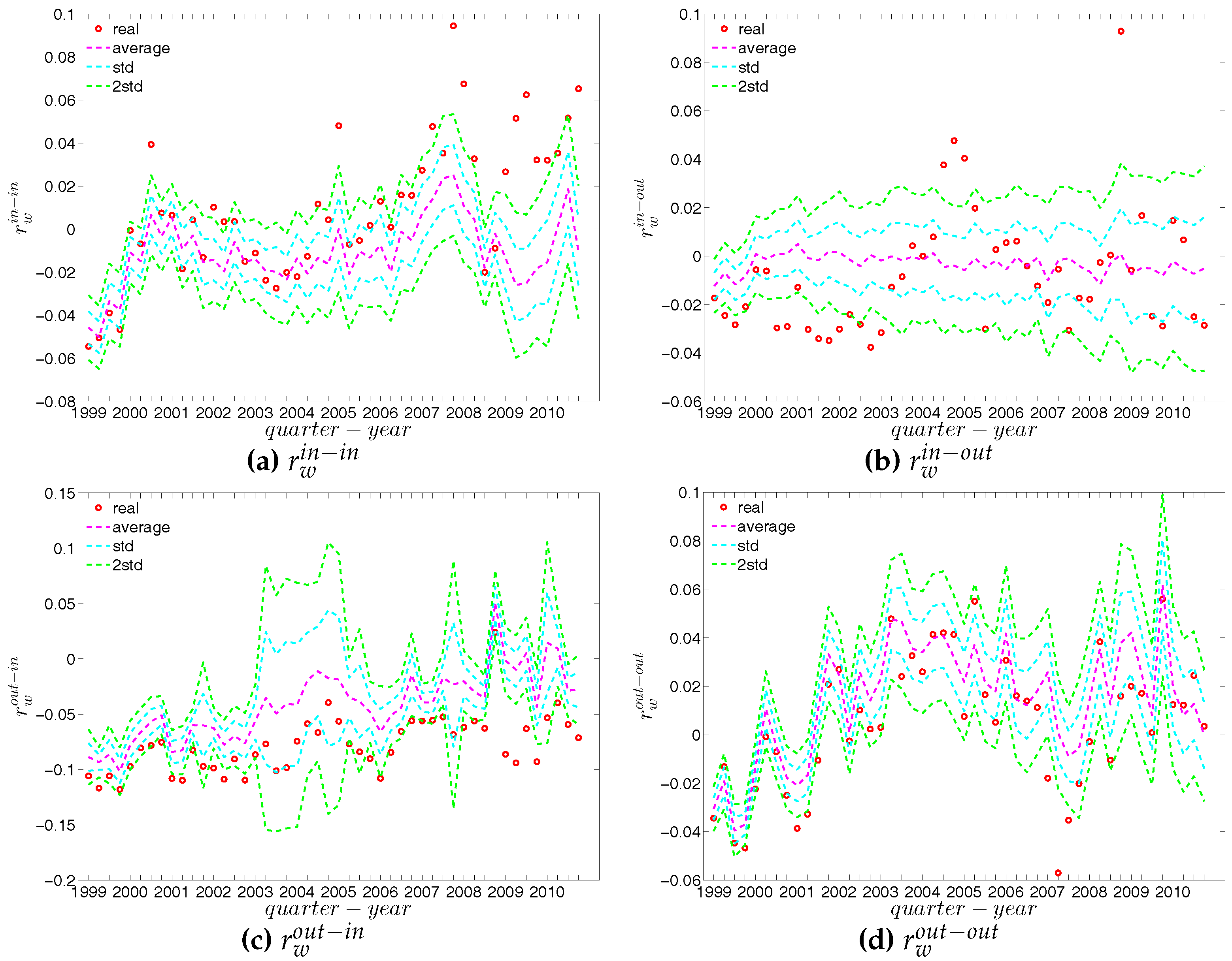
Figure 68.
Evolution of the averages of local weighted clustering coefficients in the observed e-MID network and in the DECM. (a) ; (b) ; (c) ; (d) .
Figure 68.
Evolution of the averages of local weighted clustering coefficients in the observed e-MID network and in the DECM. (a) ; (b) ; (c) ; (d) .
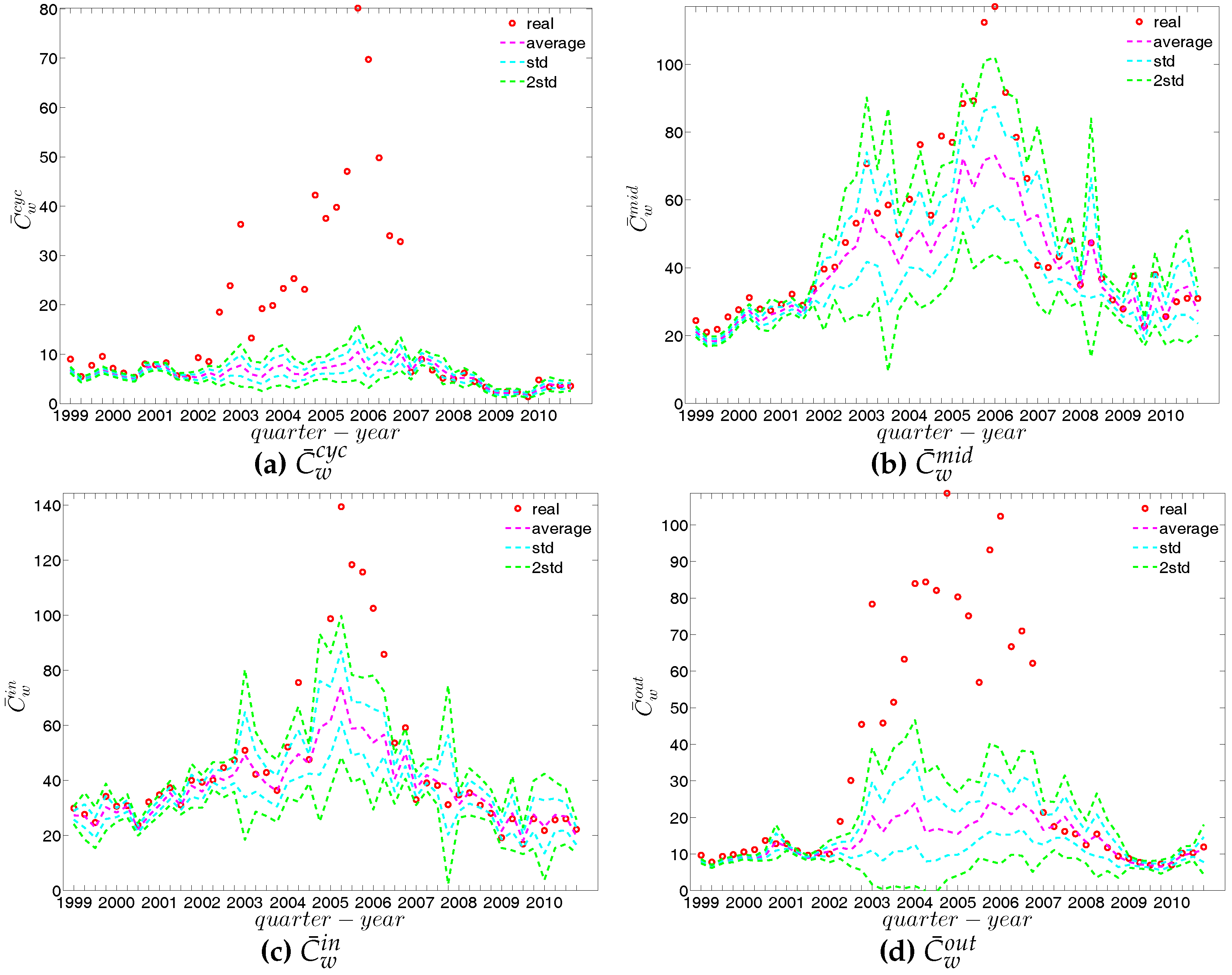
Figure 69.
Evolution of the z-scores for (a) ; (b) ; and (c) evaluated under the UWCM (red dashed lines) and the UECM (blue dashed lines).
Figure 69.
Evolution of the z-scores for (a) ; (b) ; and (c) evaluated under the UWCM (red dashed lines) and the UECM (blue dashed lines).
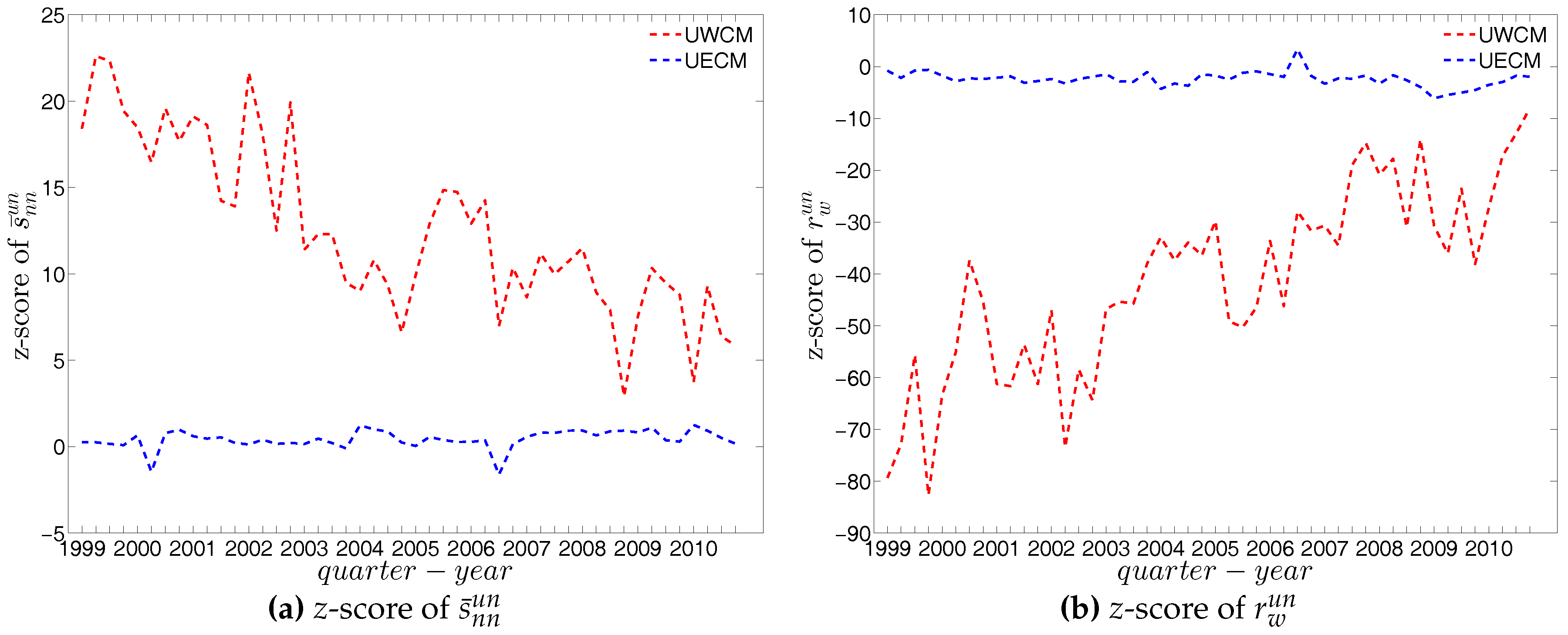
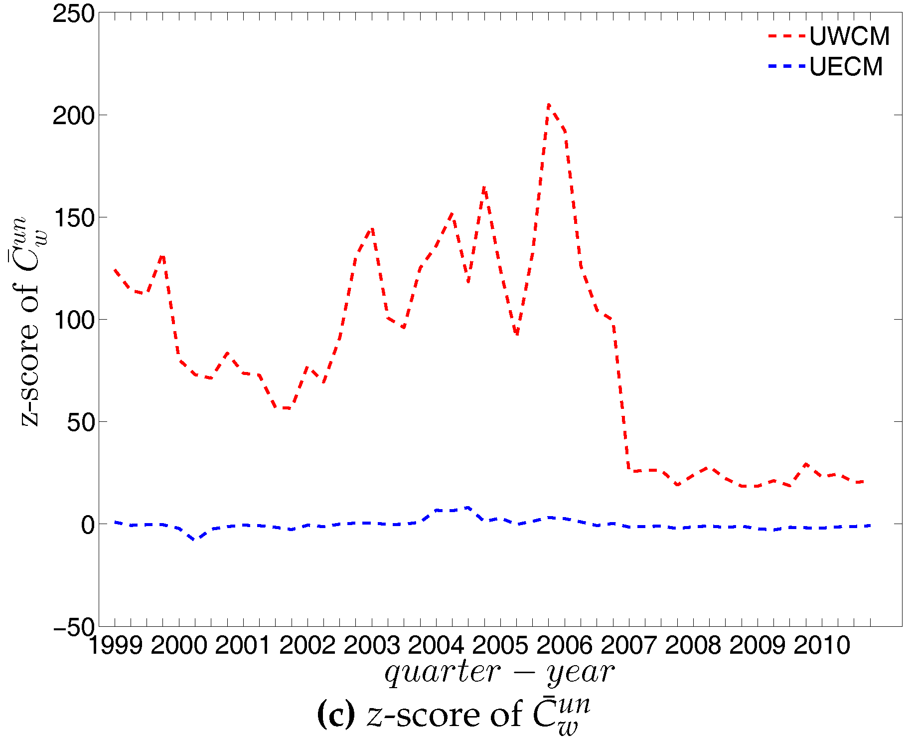
Figure 70.
Evolution of the z-scores for (a) ; (b) ; (c) , and (d) evaluated under the DWCM (red dashed lines) and the DECM (blue dashed lines).
Figure 70.
Evolution of the z-scores for (a) ; (b) ; (c) , and (d) evaluated under the DWCM (red dashed lines) and the DECM (blue dashed lines).

Figure 71.
Evolution of the z-scores for (a) ; (b) ; (c) ; and (d) evaluated under the DWCM (red dashed lines) and the DECM (blue dashed lines).
Figure 71.
Evolution of the z-scores for (a) ; (b) ; (c) ; and (d) evaluated under the DWCM (red dashed lines) and the DECM (blue dashed lines).
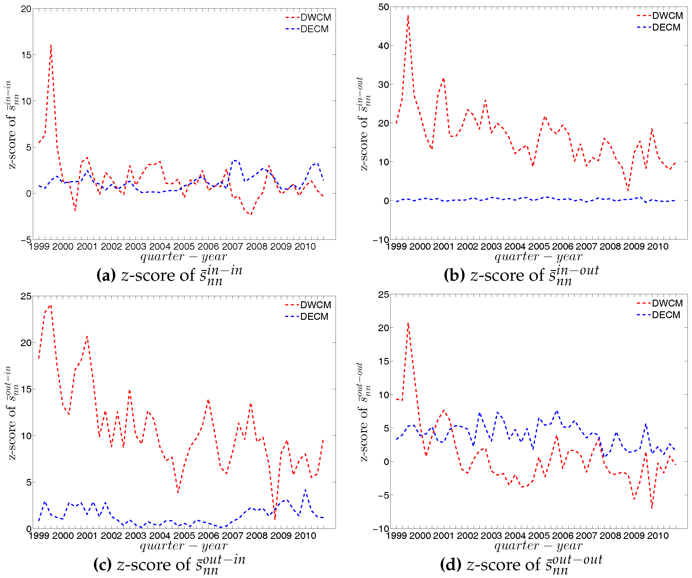
Figure 72.
Evolution of the z-scores for (a) ; (b) ; (c) ; and (d) evaluated under the DWCM (red dashed lines) and the DECM (blue dashed lines).
Figure 72.
Evolution of the z-scores for (a) ; (b) ; (c) ; and (d) evaluated under the DWCM (red dashed lines) and the DECM (blue dashed lines).

© 2017 by the authors. Licensee MDPI, Basel, Switzerland. This article is an open access article distributed under the terms and conditions of the Creative Commons Attribution (CC BY) license (http://creativecommons.org/licenses/by/4.0/).
Share and Cite
MDPI and ACS Style
Luu, D.T.; Lux, T.; Yanovski, B. Structural Correlations in the Italian Overnight Money Market: An Analysis Based on Network Configuration Models. Entropy 2017, 19, 259. https://doi.org/10.3390/e19060259
AMA Style
Luu DT, Lux T, Yanovski B. Structural Correlations in the Italian Overnight Money Market: An Analysis Based on Network Configuration Models. Entropy. 2017; 19(6):259. https://doi.org/10.3390/e19060259
Chicago/Turabian StyleLuu, Duc Thi, Thomas Lux, and Boyan Yanovski. 2017. "Structural Correlations in the Italian Overnight Money Market: An Analysis Based on Network Configuration Models" Entropy 19, no. 6: 259. https://doi.org/10.3390/e19060259
Note that from the first issue of 2016, this journal uses article numbers instead of page numbers. See further details here.