Article

Self-Organized Patterns Induced by Neimark-Sacker, Flip and Turing Bifurcations in a Discrete Predator-Prey Model with Lesie-Gower Functional Response

Research Center for Engineering Ecology and Nonlinear Science, North China Electric Power University, Beijing 102206, China
*
Author to whom correspondence should be addressed.
Entropy 2017, 19(6), 258; https://doi.org/10.3390/e19060258
Submission received: 19 April 2017 / Revised: 22 May 2017 / Accepted: 1 June 2017 / Published: 7 June 2017
(This article belongs to the Special Issue Complex Systems, Non-Equilibrium Dynamics and Self-Organisation)

Abstract

:
The formation of self-organized patterns in predator-prey models has been a very hot topic recently. The dynamics of these models, bifurcations and pattern formations are so complex that studies are urgently needed. In this research, we transformed a continuous predator-prey model with Lesie-Gower functional response into a discrete model. Fixed points and stability analyses were studied. Around the stable fixed point, bifurcation analyses including: flip, Neimark-Sacker and Turing bifurcation were done and bifurcation conditions were obtained. Based on these bifurcation conditions, parameters values were selected to carry out numerical simulations on pattern formation. The simulation results showed that Neimark-Sacker bifurcation induced spots, spirals and transitional patterns from spots to spirals. Turing bifurcation induced labyrinth patterns and spirals coupled with mosaic patterns, while flip bifurcation induced many irregular complex patterns. Compared with former studies on continuous predator-prey model with Lesie-Gower functional response, our research on the discrete model demonstrated more complex dynamics and varieties of self-organized patterns.

1. Introduction

Predator-prey systems are some of the essential ecological systems in Nature. The dynamic behaviors of the predator-prey system have captured the interest of both biologists and ecologists [1,2,3,4,5]. There are a substantial number of predator-prey system models. Recently, the formation of patterns has become a very hot topic [6,7,8,9]. This is because the formation process demonstrates self-organization of spatial heterogeneity, and shows system complexity directly and visibly. This visible complexity matches well what has been found in real ecosystems, however, the dynamics of predator-prey systems are so complex that more studies are still needed to explore the mechanism of pattern formation.
Reaction-diffusion models are commonly used to investigate spatially extended predator-prey systems [6,7,8,10,11,12,13,14]. Through Turing bifurcation, reaction-diffusion models have successfully revealed the pattern formation mechanism in many different ecosystems [2,12,13,15,16,17]. Simulations have shown a variety of patterns such as spots, stripes, labyrinth, spirals, gaps, and so on [6,10,13]. Different reaction-diffusion models focus on different functional responses that describe different predation relationships. There are a variety of responses [18], such as Lesie-Gower functional responses [19,20], Beddington-DeAngelis functional responses [14,21,22,23,24] and so on. Among these functional responses, the Leslie-Gower formulation is based on the assumption that a reduction in a predator population has a reciprocal relationship with per capita availability of its preferred food. Indeed, Leslie [19] introduced a predator-prey model where the carrying capacity of the predator is proportional to the number of its prey. This interesting formulation for predator dynamics has been discussed by Leslie and Gower [20] and Pielou [25].
In expressing predator-prey models, two main types of models are considered—continuous models and discrete models—with the latter showing more advantages in revealing complex nonlinear dynamics. A classic example is the discrete logistic model that exhibits period-doubling cascade and a route to chaos [21]. On the contrary, the continuous logistic model shows a simple “S” form curve, but never demonstrates the above dynamic complexity. Through a variety of bifurcations, discrete models can generate periodic orbits, invariant circles, periodic windows, chaotic behavior and so on. More importantly, in predator-prey systems, births and deaths of bionts are discrete events, which means continuous models only make sense for very large populations. Many researchers think that discrete models can reveal the discontinuous properties (such as a patchy environment or a fragmented habitat) of predator-prey systems [26]. Besides, discrete models may exhibit new dynamic behaviors. For example, Han et al. found that Turing instability and Turing patterns can occur in a simple discrete competitive Lotka-Volterra system rather than the continuous one [27].
In this research, we will transform a well-recognized continuous predator-prey model into a discrete model. The continuous model incorporates the Holling-type-II and the modified Lesie-Gower functional responses, that can be shown as:
{ H T = ( a 1 b 1 H c 1 P H + k 1 ) H + D 1 ( 2 H X 2 + 2 H Y 2 ) P T = ( a 2 c 2 P H + k 2 ) P + D 2 ( 2 P X 2 + 2 P Y 2 )
where H and P are the densities of prey and predators, respectively. (X,Y) is the spatial position of species when they move in a two dimensional space. D1 and D2 are the diffusion coefficients of prey and predator respectively. a1 is the growth rate of prey H. a2 describes the growth rate of predator P. b1 measures the strength of competition among individuals of species H. c1 is the maximum value of the per capita reduction of H due to P. c2 has a similar meaning to c1. k1 measures the extent to which environment provides protection to prey H. k2 has a similar meaning to k1 relatively to the predator P. With scaling transformations:
t = a 1 T ,   u ( t ) = b 1 a 1 H ( T ) ,   v ( t ) = c 2 b 1 a 1 a 2 P ( T ) ,   x = X ( a 1 D 1 ) 1 2 ,   y = Y ( a 1 D 1 ) 1 2 a = a 2 c 1 a 1 c 2 ,   b = a 2 a 1 ,   e 1 = b 1 k 1 a 1 ,   e 2 = b 1 k 2 r 1 ,   δ = D 2 D 1 ,
the continuous model can be expressed as:
{ u t = 2 u x 2 + 2 u y 2 + u ( 1 u ) a u v u + e 1 = 2 u x 2 + 2 u y 2 + f ( u , v ) v t = δ ( 2 v x 2 + 2 v y 2 ) + b ( 1 v u + e 2 ) v = δ ( 2 v x 2 + 2 v y 2 ) + g ( u , v ) .
The local dynamics of this continuous model (3) has been studied in [28,29], and the global stability of a similar model has been investigated in [30]. A similar model with delay is studied in [31,32], and a three dimensional similar model with the same functional responses is studied in [33,34,35]. In [36], several Turing and Hopf bifurcation patterns were obtained by the continuous model (3). We can see that this model is well recognized.
A few researchers found that more complex dynamics could be generated through discretizing the continuous model [26,37,38,39,40]. Based on the approach in prior studies [26,37,38,39], here we investigated the complex dynamics via transforming the continuous model (3) to a discrete model. In the analysis of the discrete model, fixed points and stability analysis were studied. Three types of bifurcation analysis were conducted, including flip bifurcation, Neimark-Sacker bifurcation and Turing bifurcation. Then numerical simulations were carried out under these bifurcation conditions, to show the complex dynamics and the formation self-organized patterns with this discrete model. Discussions focused on the types of self-organized patterns, and the relations between bifurcations and pattern types.

2. Model and Stability Analysis

2.1. A Discrete Predator-Prey Model

In this research, the above continuous model Equation (3) will be transformed to a discrete model. We consider the model on a N × N lattice, and the two variables can be expressed as u(i,j,t) and v(i,j,t) (i,j ∈ {1,2,3,…N} and tZ+), that represent the prey density and the predator density in lattice (i,j) at time t, respectively. According to the former research works of [26,37,38,39], there are two stages, reaction stage and diffusion stage, when we discretize the continuous model (3). The diffusion stage is considered firstly as:
{ u ( i , j , t ) = u ( i , j , t ) + τ h 2 d 2 u ( i , j , t ) v ( i , j , t ) = v ( i , j , t ) + τ h 2 δ d 2 v ( i , j , t ) ,
where τ and h are the time interval and space interval. d 2 denotes the discrete form of the Laplacian operator. Note that the whole research is using periodic boundary conditions. Then we consider the reaction stage:
{ u ( i , j , t + 1 ) = f 1 ( u ( i , j , t ) , v ( i , j , t ) ) v ( i , j , t + 1 ) = g 1 ( u ( i , j , t ) , v ( i , j , t ) ) ,
in which:
{ f 1 ( u , v ) = u + τ f ( u , v ) g 1 ( u , v ) = v + τ g ( u , v ) .
Equations (4)–(6) including both diffusion and reaction stages are defined as our discrete model.

2.2. Fixed Points and Stability

As we obtain a new discrete model, fixed points and stability analysis need to be investigated. The fixed points should satisfy:
d 2 u ( i , j , t ) = d 2 v ( i , j , t ) = 0 .
Then we get:
{ u ( i , j , t ) = u ( i , j , t ) v ( i , j , t ) = v ( i , j , t ) ,
and:
{ u ( i , j , t + 1 ) = f 1 ( u ( i , j , t ) , v ( i , j , t ) ) v ( i , j , t + 1 ) = g 1 ( u ( i , j , t ) , v ( i , j , t ) ) .
The above equation can be expressed as the following map:
( u v ) ( u + τ u ( 1 u ) τ a u v u + e 1 v + τ b ( 1 v u + e 2 ) v ) .
Thus the fixed points of the map can be shown as:
( u 1 , v 1 ) = ( 0 , 0 ) ,
( u 2 , v 2 ) = ( 0 , e 2 ) ,
( u 3 , v 3 ) = ( 1 , 0 ) ,
( u 4 , v 4 ) = ( u , v ) .
in which, (u*,v*) is the positive solution of the following equations:
{ u 2 + ( a + e 1 1 ) u + a e 2 e 1 = 0 v = u + e 2 .
Therefore, the sufficient and necessary condition of u* > 0, v* > 0 can be obtained as:
( a + e 1 1 ) 2 4 ( a e 2 e 1 ) > 0 ,   1 a e 1 + ( a + e 1 1 ) 4 ( a e 2 e 1 ) > 0 .
The stability of the fixed points can be studied through a Jacobi matrix with spatially homogeneous perturbations, that is shown as:
J = [ 1 + τ [ 1 2 u a v e 1 ( u + e 1 ) 2 ] τ a u u + e 1 τ b v 2 ( u + e 2 ) 2 1 + τ ( b 2 b v u + e 2 ) ] .
Substituting (u1,v1) into J, we can get:
J | ( u 1 , v 1 ) = [ 1 + τ 0 0 1 + τ b ] .
As 1 + τ > 1, 1 + τb > 1, thus (u1,v1) is unstable. Substituting ( u 2 , v 2 ) into J , we can get:
J | ( u 2 , v 2 ) = [ 1 + τ ( 1 a e 2 e 1 ) 0 τ b 1 τ b ] .
When 1 < ae2/e1 < 1 + 2/τ and 0 < b < 2/τ, (u2,v2) is stable. Substituting (u3,v3) into J, we can get:
J | ( u 3 , v 3 ) = [ 1 τ τ a 1 + e 1 0 1 + τ b ] .
The stability requires | 1 τ | < 1 and | 1 + τ b | < 1 , that is 0 < τ < 2 and τ < 0 . But this is a contradiction. Thus ( u 3 , v 3 ) is unstable.
Substituting ( u 4 , v 4 ) into J , we can get:
J | ( u 4 , v 4 ) = [ a 11 a 12 a 21 a 22 ] .
In which:
a 11 = 1 + τ [ 1 2 u a ( u + e 2 ) e 1 ( u + e 1 ) 2 ] ,   a 12 = τ a u u + e 1 ,   a 21 = τ b ,   a 22 = 1 τ b
Let:
t r 0 = a 11 + a 22 ,
Δ 0 = a 11 a 22 a 12 a 21 .
The eigenvalues can be obtained as:
λ 1 , 2 = t r 0 ± t r 0 2 4 Δ 0 2 .
Therefore ( u 4 , v 4 ) is stable only when:
{ Δ 0 < 1 ( 1 + Δ 0 ) < t r 0 < 1 + Δ 0 .

2.3. Bifurcation Analysis

In this subsection, we focus on the bifurcation analysis at fixed point (u4,v4). Parameter conditions of three bifurcations are obtained, including Neimark-Sacker bifurcation, flip bifurcation and Turing bifurcation. The detailed progress of each bifurcation analysis is shown in Appendix A.

3. Numerical Simulations

Simulations will be carried out for each bifurcation calculated in Section 2.3. (Appendix A). Bifurcation diagrams and phase portraits will be shown to interpret the system dynamics when Neimark-Sacker bifurcation or flip bifurcation conditions occur. The emergence of Turing bifurcation is also demonstrated by simulating the variations of eigenvalues (curve of Equation (A43)). And then self-organized patterns will be shown with the corresponding parameters under each bifurcation condition.

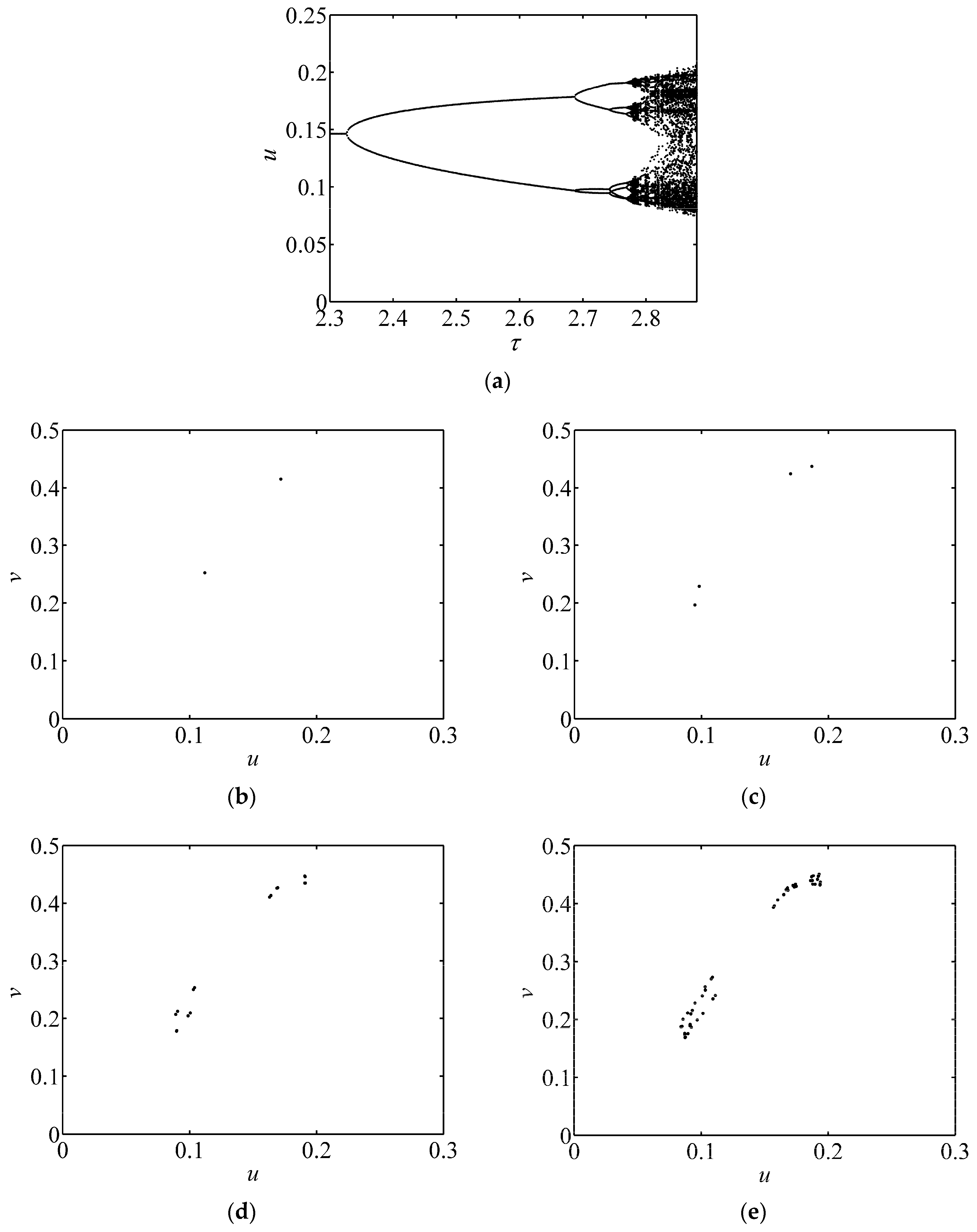
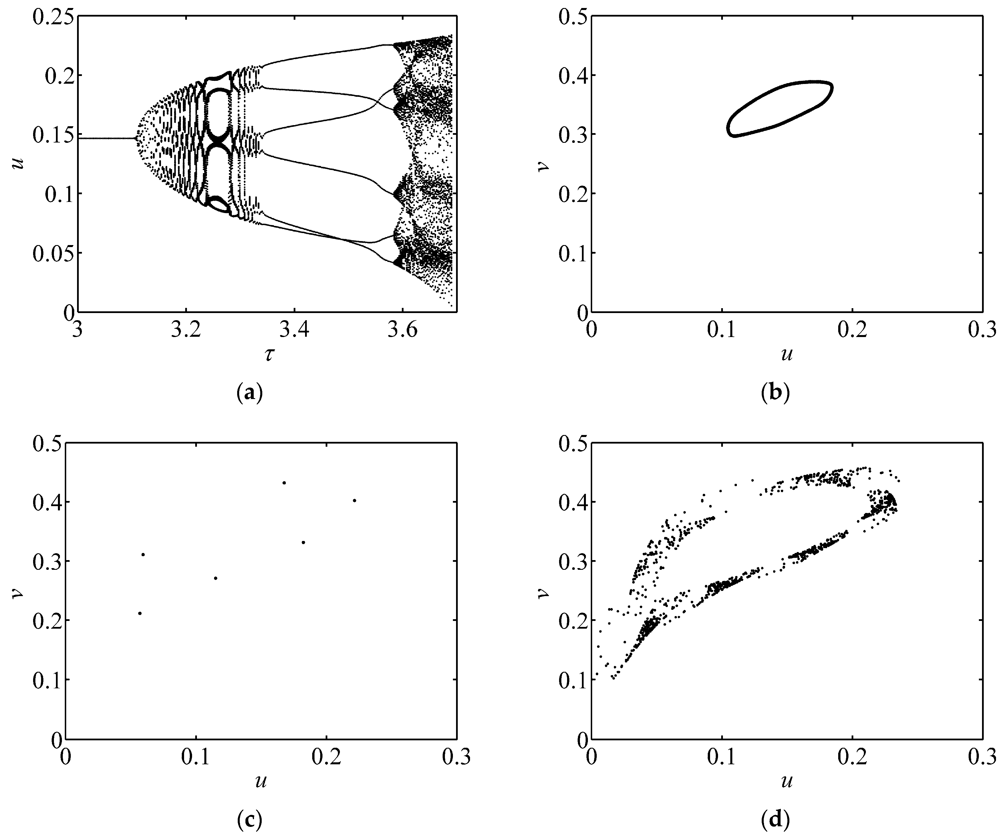
3.1. Bifurcation Diagram and Phase Portrait

Figure 1 shows variations of u versus the parameter τ when the parameter values satisfy the flip bifurcation conditions. When τ > 2.3267, the fixed point is asymptotically stable. When τ = 2.3267, the system starts to bifurcate around a fixed point. With the increase of τ , the stable states of the system go through (not only these states) period-2 (τ = 2.5 as shown in Figure 1b), period-4 (τ = 2.72 as shown in Figure 1c), period-10 (τ = 2.77 as shown in Figure 1d) and then complex periodic oscillations (τ = 2.83 as shown in Figure 1e).
Figure 2 shows the variations of u versus parameter τ when the parameter values satisfy the Neimark-Sacker bifurcation conditions. Note that this bifurcation diagram has no visible periodic windows. When τ < 2.8291, the fixed point is asymptotically stable. When τ = 2.8291, the system starts to bifurcate around a fixed point. With the increase of τ, the states of the system increase, but the system always follows the invariant circle. For example, when τ = 3, Figure 2b shows how the bifurcation drives the system from a fixed point (with 1% random perturbations) to the invariant circle in the phase plane (u,v).
Figure 3 shows another Neimark-Sacker bifurcation situation. Note that this bifurcation diagram has several periodic windows. When τ < 3.1087, the fixed point is asymptotically stable and the bifurcation point of the system is determined at τ = 2.1087.
As the value of τ increases, the stable states of the system experience several stages, such as invariant circle (τ = 3.1750 as shown in Figure 3b), period-6 (τ = 3.5250 as shown in Figure 3c), and then invariant circle again (τ = 3.69 as shown in Figure 3d).
Turing bifurcation can be shown through the variations of eigenvalues λ(k,l) as shown in Figure 4. In Figure 4a, we can see that the effects of the perturbation numbers k and l are symmetric. Thus we let k = l, and we can get the variations of eigenvalues versus l as shown in Figure 4b. When there is no perturbation, the system stays at the fixed point. When the diffusion coefficient δ = 2, the eigenvalues of the system remain at less than 1 with the increase of perturbation number l. But when the diffusion coefficient δ increases more than δc, the eigenvalues will exceed 1 with the increase of l and Turing bifurcation occurs.

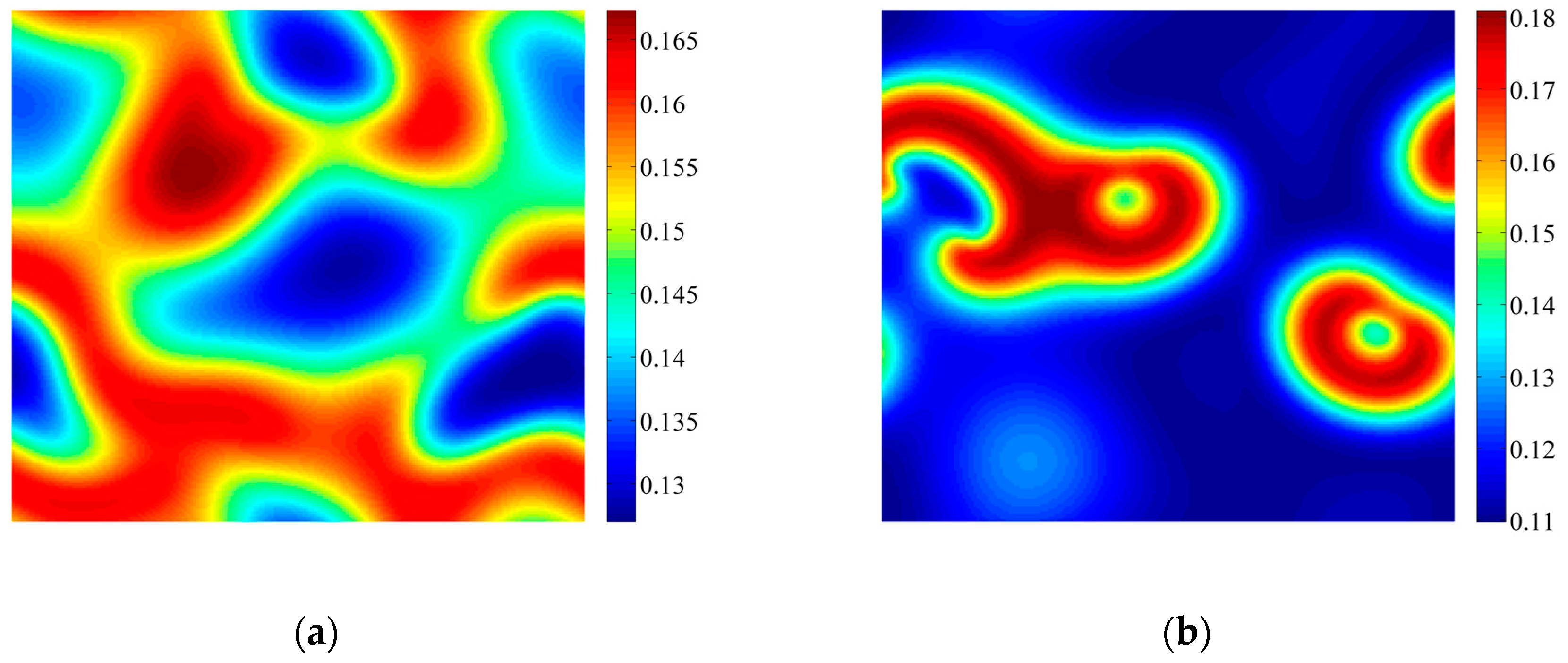
3.2. Formation of Self-Organized Patterns

In order to investigate the formation of self-organized patterns under the above bifurcation conditions, simulations will be carried out on 100 × 100 lattices with periodic boundary conditions. Initial conditions are set as fixed points with heterogeneous random disturbance (1%). Given the parameter values under each bifurcation condition, the formation of patterns can be obtained after t = 2000. Patterns will be shown only in terms of variable u, as the patterns of variable v are similar.
Figure 5 shows the patterns induced by Neimark-Sacker bifurcation. The parameters a = 1.1, e1 = 0.3, e2 = 0.2, b = 0.3739 and τ = 2.84 satisfy the Neimark-Sacker bifurcation conditions. We can see that spot patterns are formed through self-organization of variable u. With the increase of τ, the patterns become more isolated.
Figure 6 shows the patterns of variable u induced by Neimark-Sacker bifurcation. Parameters a = 1.1, e1 = 0.3, e2 = 0.2, b = 0.373 and τ satisfy the Neimark-Sacker bifurcation conditions. We can see that with the increase of τ, patterns are formed through the self-organization of u. Moreover, these patterns transit from the irregular pattern in Figure 6a to spiral patterns in Figure 6b–d, and the wavelength of the spirals decreases gradually. Spiral patterns are some of the patterns that are often recorded in the studies of predator-prey systems [41].
Figure 7 shows the patterns of variable u induced by Turing bifurcation. Parameters a = 1.1, e1 = 0.3, e2 = 0.2, b = 0.1781 and τ = 0.1, 0.2 do not satisfy Neimark-Sacker bifurcations or flip bifurcation conditions, but the addition of δ = 30 and h = 6 make Turing bifurcation occur. We can see that a labyrinth pattern is formed through the self-organization of u. With the increase of τ, the stripes in the labyrinth pattern become broader.
Figure 8 shows the pattern of variable u induced by Turing bifurcation. Parameters a = 1.1, e1 = 0.3, e2 = 0.2, b = 0.3739 and τ = 2.8, 2.82 do not satisfy Neimark-Sacker bifurcations or flip bifurcation conditions, but addition of δ = 3.2 and h = 6 make Turing bifurcation occur. We can see that complex patterns are formed through the self-organization of u. The parameter values of Figure 7 and Figure 8 both satisfy the Turing bifurcation conditions, but the types are quite different from each other. The patterns in Figure 8 are like spiral patterns coupled with irregular mosaics. Note that the patterns in Figure 8 are similar as those in Figure 6. The reason may be that the value of τ is very close to the Neimark-Sacker bifurcation point, that is τ = 2.8291.
Figure 9 shows the pattern induced by flip bifurcation. Parameters a = 1.1, e1 = 0.3, e2 = 0.2, b = 1.2 and τ satisfy the flip bifurcation conditions. We can see that patterns are formed through the self-organization of variable u. The type of pattern is quite difficult to define, but they can be reflected by the phase portrait above, that are similar to those in Figure 1. Figure 9a–d show the patterns generated by period-2, period-4, period-6 and multi-period behaviors. Due to the effect of period-doubling cascade, patterns become more and more fractal.

4. Discussion and Conclusions

We have transformed a well-recognized continuous predator-prey model into a discrete model. During the transformation, the iteration process is considered in two stages: diffusion stage and then reaction stage. Fixed points and stability analysis are studied. Three types of bifurcation analysis are performed for the discrete model, including flip bifurcation, Neimark-Sacker bifurcation, and Turing bifurcation. With parameter values satisfying bifurcation conditions, numerical simulations are carried out to show the self-organized patterns of the predator-prey model.
From the pattern simulations, we can see that Turing instability leads to the formation of spatial patterns of labyrinth and complex patterns of spirals coupled with mosaics, Neimark-Sacker bifurcation induces the formation of spots and spiral patterns, and flip bifurcation induces the formation of irregular patterns corresponding to period-2, period-4 and many complex periodic behaviors. We can see that these patterns are quite different from each other, which shows the distinguishing effects of these three types of instabilities (based on three bifurcation situations).
These self-organized patterns can also be classified into two categories: stationary patterns and oscillatory patterns. Oscillatory patterns include the spiral patterns, and stationary patterns include the other patterns. In the stationary patterns, the spatial distribution of predator and prey remains stationary and the system dynamics will not change with time. In the oscillatory patterns, the dynamics of predator and prey is always varying spatially and temporally as time goes on. One of important characteristics of the oscillatory patterns is spatiotemporal chaos, which results in the formation of complex and diverse spiral patterns.
Compared with previous studies on a continuous predator-prey model with Lesie-Gower functional response [36], the simulations on our discrete model with same functional response show not only that all the patterns were obtained by the continuous model, but also many special patterns can be induced by flip bifurcation and a special type of pattern is induced by Turing bifurcation. This proves that discrete models can generate more self-organized patterns. The most important reason is, especially in our model, the import of time interval τ gives more possibility to the system to generate these complex dynamics. Furthermore, we think the variations of τ reflect the multiple time scale in the real ecosystems. The conclusions of this research can be summarized as follows:
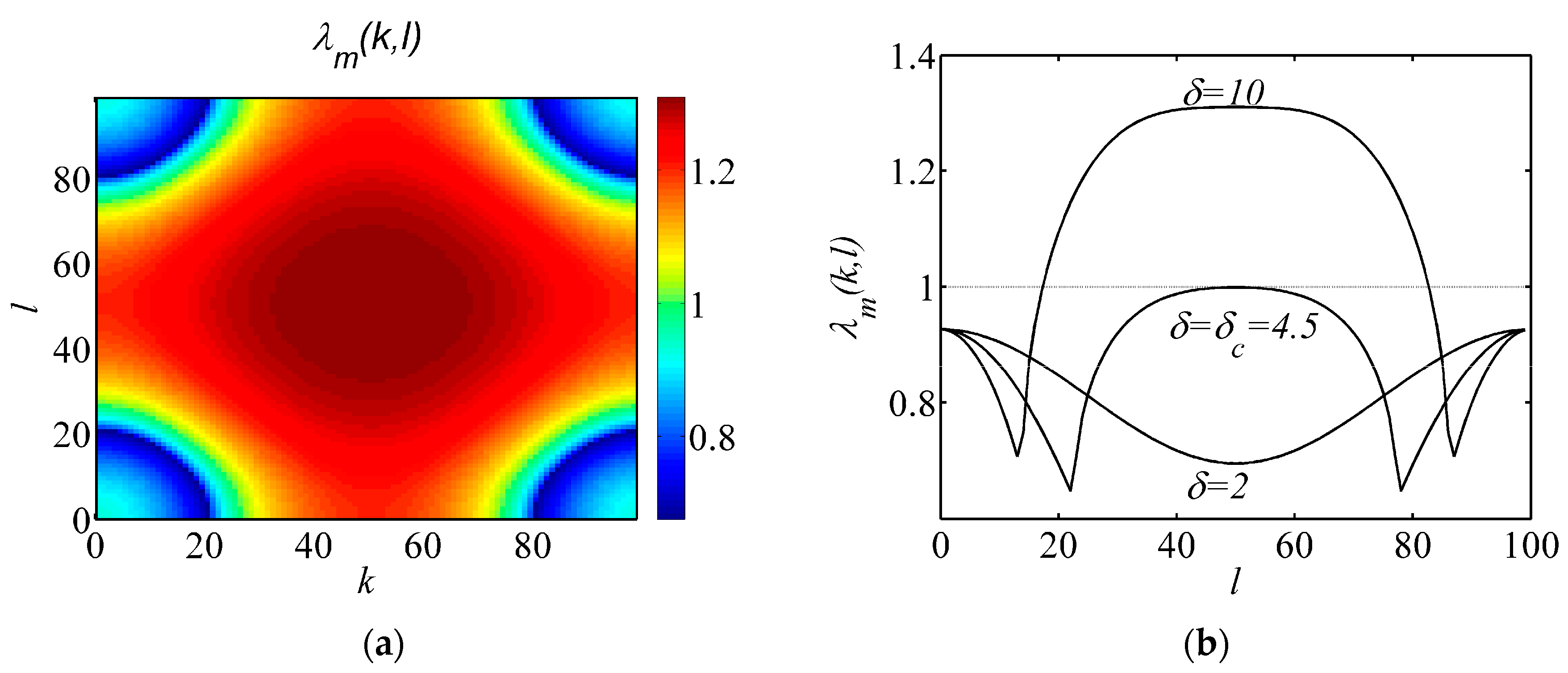
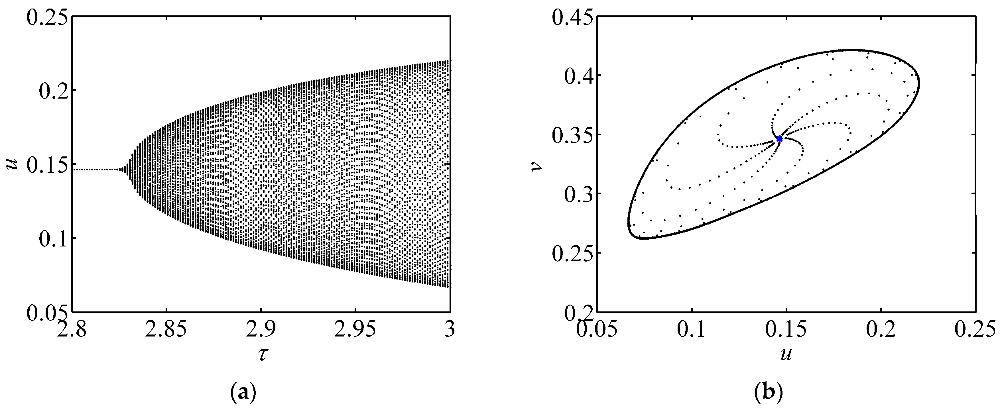
  • The discrete predator-prey model with Lesie-Gower functional response can generate many complex dynamics including three types of bifurcations, which are flip bifurcation, Neimark-Sacker bifurcation and Turing bifurcation.
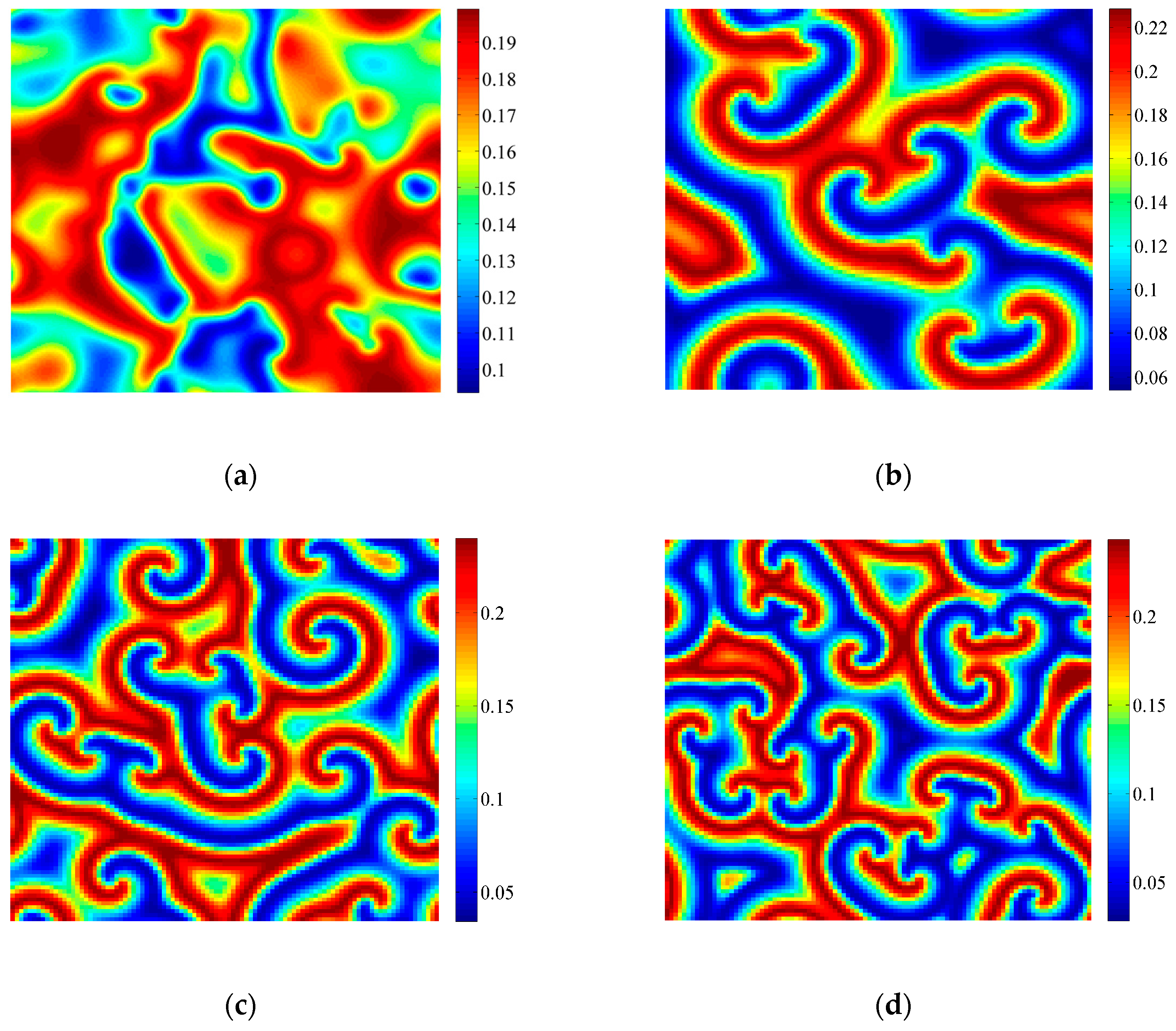
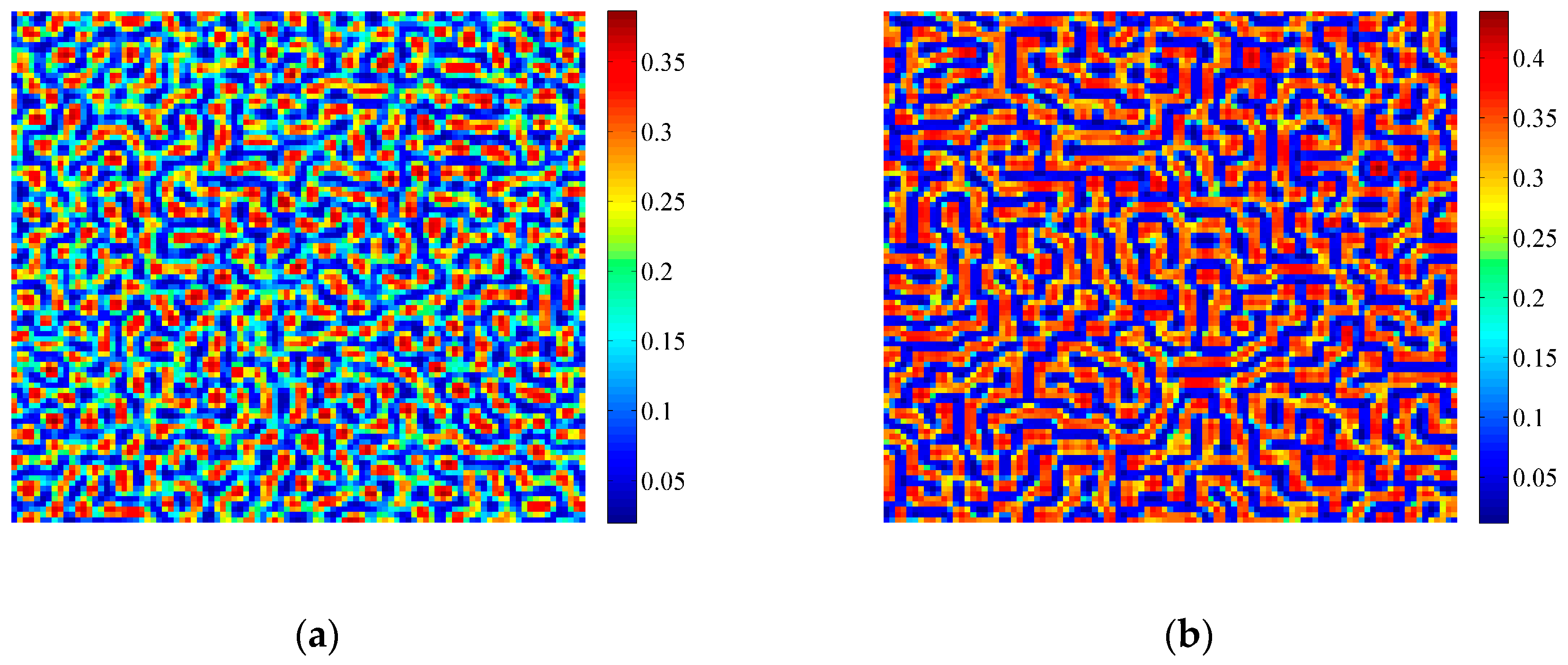
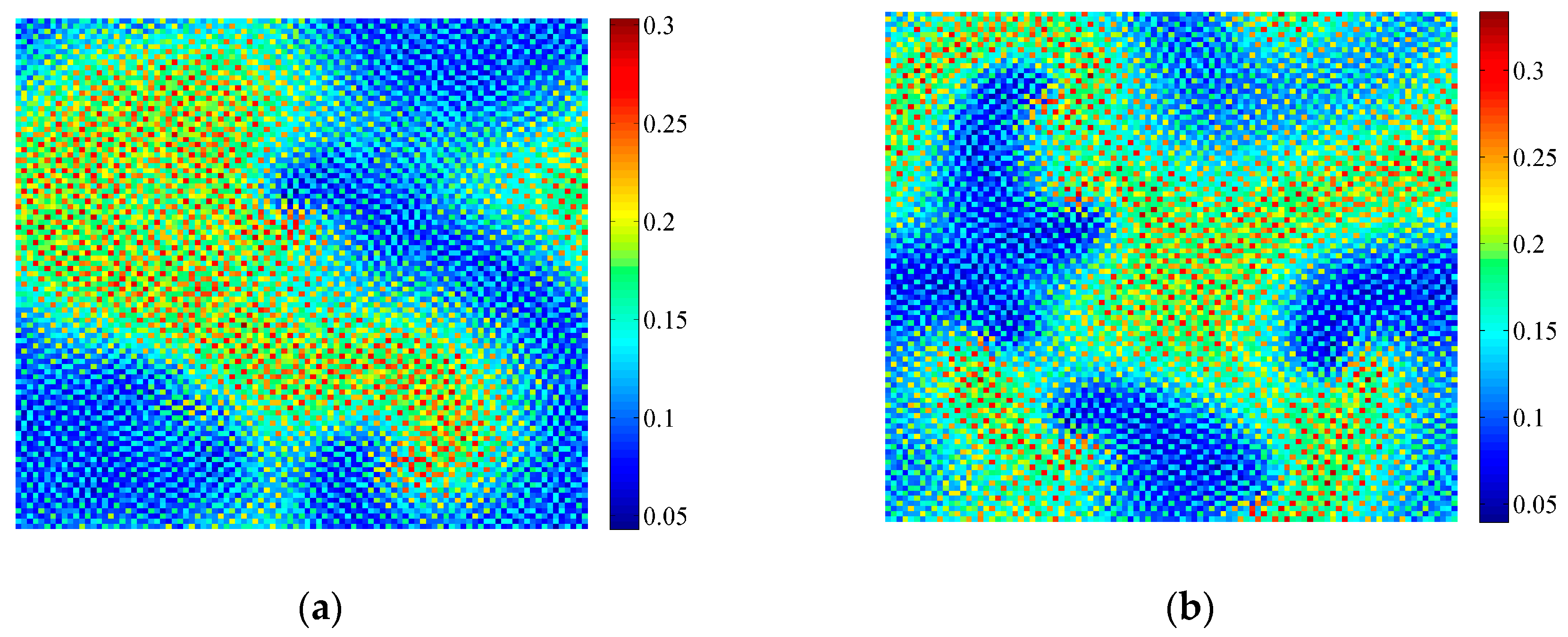
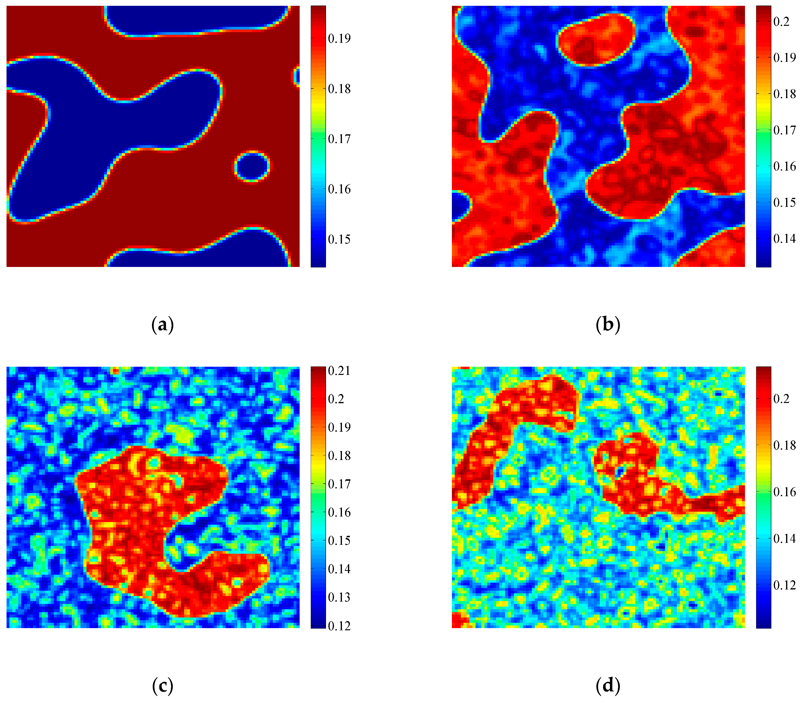
  • A variety of self-organized patterns can be formed through the discrete predator-prey model with Lesie-Gower functional response and the above three bifurcations. These patterns consist of spots, transitional patterns from spots to spirals, spirals, spirals coupled with mosaics, labyrinths, and many other complex patterns generated by flip bifurcation.
  • Among the studies on predator-prey models with Lesie-Gower functional response, this research may develop a special perspective to interpret the how self-organized patterns are generated.

Acknowledgments

The authors would like to acknowledge with great gratitude for the supports of Chinese Natural Science Foundation (Project 39560023 to Huayong Zhang), National Special Water Programs (No. 2009ZX07210-009, No. 2015ZX07203-011, No. 2015ZX07204-007), Department of Environmental Protection of Shandong Province (SDHBPJ-ZB-08). The authors would thank Jennifer Swann from USA for the language checking.

Author Contributions

Huayong Zhang and Tousheng Huang proposed the idea. Shengnan Ma, Tianxiang Meng and Hongju Yang calculated the fixed points and stability analysis and verified the bifurcation conditions. Feifan Zhang did all the bifurcation conditions, simulations and wrote the paper.

Conflicts of Interest

The authors declare no conflict of interest.

Appendix A

Appendix A.1. Flip Bifurcation Analysis

The occurrence of flip bifurcation [42] requires one of the two eigenvalues of J | ( u 4 , v 4 ) satisfies λ = −1. If we give Δ0 = −tr0 − 1, in which:
Δ 0 = a 11 a 22 a 12 a 21 = 1 + τ A τ + τ B τ 2 ,
τ A = 1 2 u a ( u + e 2 ) e 1 ( u + e 1 ) 2 b ,
τ B = [ 1 2 u a e 1 ( u + e 2 ) ( u + e 1 ) 2 ] ( b ) + a b u ( u + e 1 ) .
Equations (A1)–(A3) lead to:
τ 0 = 4 τ A + τ A 2 4 τ B ,
or:
τ 0 = 4 τ A τ A 2 4 τ B .
The two eigenvalues of J ( u 3 , v 3 ) become λ 1 = 1 and λ 2 = 1 + t r 0 ( τ 0 ) . Meanwhile, the occurrence of flip bifurcation requires | λ 2 | 1 , that is:
τ 0 ( 1 2 u a ( u + e 2 ) e 1 ( u + e 1 ) 2 b ) 2 ,   4 .
Considering τ as a dependent variable, and let:
x = u u ,   y = v v ,   τ ˜ = τ τ 0 ,
we can get a new map:
( x y τ ˜ ) ( a 11 x + a 12 y + a 13 2 x 2 + a 14 x y + a 15 x τ ˜ + a 16 y τ ˜ + a 17 6 x 3 + a 18 2 x 2 y + a 19 2 x 2 τ ˜ + a 110 x y τ ˜ + O ( ( | x | + | y | + | τ ˜ | ) 4 ) a 21 x + a 22 y + a 23 2 x 2 + a 24 2 y 2 + a 25 x y + a 26 x τ ˜ + a 27 y τ ˜ + a 28 6 x 3 + a 29 2 x 2 y + a 210 2 x y 2 + a 211 2 x 2 τ ˜ + a 212 2 y 2 τ ˜ + a 213 x y τ ˜ + O ( ( | x | + | y | + | τ ˜ | ) 4 ) τ ˜ ) .
where O ( ( | x | + | y | + | τ ˜ | ) 4 ) is a function with at least four order in the variables ( x , y , τ ˜ ) , and:
a 11 = 1 + τ ( 1 2 u a e 1 ( u + e 2 ) ( u + e 1 ) 2 ) ,   a 12 = a τ u u + e 1 ,   a 13 = 2 τ ( 1 + a e 1 ( u + e 2 ) ( u + e 1 ) 3 ) ,
a 14 = a e 1 τ ( u + e 1 ) 2 ,   a 15 = 1 2 u a e 1 ( u + e 2 ) ( u + e 1 ) 2 ,   a 16 = a u u + e 1 , a 17 = 6 τ a e 1 ( u + e 2 ) ( u + e 1 ) 4 ,
a 18 = 2 a e 1 τ ( u + e 1 ) 3 ,   a 19 = 2 + 2 a e 1 ( u + e 2 ) ( u + e 1 ) 3 ,   a 110 = a e 1 ( u + e 1 ) 2 ,
a 21 = b τ ,   a 22 = 1 b τ ,   a 23 = 2 b τ u + e 2 ,   a 24 = 2 b τ u + e 2 ,   a 25 = 2 b τ u + e 2 ,   a 26 = b ,
a 27 = b ,   a 28 = 6 b τ ( u + e 2 ) 2 ,   a 29 = 4 b τ ( u + e 2 ) 2 ,   a 210 = 2 b τ ( u + e 2 ) 2 ,   a 211 = 2 b u + e 2 ,
a 212 = 2 b u + e 2 ,   a 213 = 2 b u + e 2 .
According to Guckenheimer and Holmes [42], an effective method for bifurcation analysis is by applying the center manifold theorem, that enables us to restrict our attention to the flow within the center manifold, but we need to transform the map to the normal form. Applying the invertible transformation:
( x y ) = ( a 12 a 12 1 a 11 λ 2 a 11 ) ( x ˜ y ˜ ) ,
we can get:
( x ˜ y ˜ τ ˜ ) ( 1 0 0 0 λ 2 0 0 0 1 ) ( x ˜ y ˜ τ ˜ ) + 1 a 12 ( 1 + λ 2 ) ( F 1 ( x ˜ , y ˜ , τ ˜ ) F 2 ( x ˜ , y ˜ , τ ˜ ) 0 ) .
in which:
F 1 ( x ˜ , y ˜ , τ ˜ ) = a 12 2 ( a 13 ( λ 2 a 11 ) 2 a 12 a 23 2 ) ( x ˜ + y ˜ ) 2 a 12 a 24 2 ( ( 1 + a 11 ) x ˜ ( λ 2 a 11 ) y ˜ ) 2 a 12 ( a 14 ( λ 2 a 11 ) a 12 a 25 ) ( x ˜ + y ˜ ) ( ( 1 + a 11 ) x ˜ ( λ 2 a 11 ) y ˜ ) + a 12 ( a 15 ( λ 2 a 11 ) a 12 a 26 ) ( x ˜ τ ˜ + y ˜ τ ˜ ) ( a 16 ( λ 2 a 11 ) a 12 a 27 ) ( ( 1 + a 11 ) x ˜ τ ˜ ( λ 2 a 11 ) y ˜ τ ˜ ) + a 12 3 ( a 17 ( λ 2 a 11 ) 6 a 12 a 28 6 ) ( x ˜ + y ˜ ) 3 a 12 2 ( a 18 ( λ 2 a 11 ) 2 a 12 a 29 2 ) ( x ˜ + y ˜ ) 2 ( ( 1 + a 11 ) x ˜ ( λ 2 a 11 ) y ˜ ) a 12 2 a 210 2 ( x ˜ + y ˜ ) ( ( 1 + a 11 ) x ˜ ( λ 2 a 11 ) y ˜ ) 2 + a 12 2 ( a 19 ( λ 2 a 11 ) 2 a 12 a 211 2 ) ( x ˜ + y ˜ ) 2 τ ˜ a 12 a 212 2 ( ( 1 + a 11 ) x ˜ ( λ 2 a 11 ) y ˜ ) 2 τ ˜ a 12 ( a 110 ( λ 2 a 11 ) a 12 a 213 ) ( x ˜ τ ˜ + y ˜ τ ˜ ) ( ( 1 + a 11 ) x ˜ ( λ 2 a 11 ) y ˜ ) + O ( ( | x ˜ | + | y ˜ | + | τ ˜ | ) 4 ) ,
F 2 ( x ˜ , y ˜ , τ ˜ ) = a 12 2 ( a 13 ( 1 + a 11 ) 2 + a 12 a 23 2 ) ( x ˜ + y ˜ ) 2 + a 12 a 24 2 ( ( 1 + a 11 ) x ˜ ( λ 2 a 11 ) y ˜ ) 2 ( a 14 ( 1 + a 11 ) + a 12 a 25 ) ( a 12 ( x ˜ + y ˜ ) ) ( ( 1 + a 11 ) x ˜ ( λ 2 a 11 ) y ˜ ) + a 12 ( a 15 ( 1 + a 11 ) + a 12 a 26 ) ( x ˜ τ ˜ + y ˜ τ ˜ ) ( a 16 ( 1 + a 11 ) + a 12 a 27 ) ( ( 1 + a 11 ) x ˜ τ ˜ ( λ 2 a 11 ) y ˜ τ ˜ ) + a 12 3 ( a 17 ( 1 + a 11 ) 6 + a 12 a 28 6 ) ( x ˜ + y ˜ ) 3 a 12 2 ( a 18 ( 1 + a 11 ) 2 + a 12 a 29 2 ) ( x ˜ + y ˜ ) 2 ( ( 1 + a 11 ) x ˜ ( λ 2 a 11 ) y ˜ ) + a 12 2 a 210 2 ( x ˜ + y ˜ ) ( ( 1 + a 11 ) x ˜ ( λ 2 a 11 ) y ˜ ) 2 + a 12 2 ( a 19 ( 1 + a 11 ) 2 + a 12 a 211 2 ) ( x ˜ + y ˜ ) 2 τ ˜ + a 12 a 212 2 ( ( 1 + a 11 ) x ˜ ( λ 2 a 11 ) y ˜ ) 2 τ ˜ a 12 ( a 110 ( 1 + a 11 ) + a 12 a 213 ) ( x ˜ τ ˜ + y ˜ τ ˜ ) ( ( 1 + a 11 ) x ˜ ( λ 2 a 11 ) y ˜ ) + O ( ( | x ˜ | + | y ˜ | + | τ ˜ | ) 4 ) .
The center manifold W C ( 0 , 0 , 0 ) of (A10) at the fixed point ( 0 , 0 , 0 ) is then determined. According to the center manifold theorem [42], a center manifold W C ( 0 , 0 , 0 ) exists and can be approximately represented by the following expression:
W C ( 0 , 0 , 0 ) = { ( x ˜ , y ˜ , τ ˜ ) R 3 | y ˜ = h ( x ˜ , τ ˜ ) , h ( 0 , 0 ) = 0 , D h ( 0 , 0 ) = 0 } ,
where h ( x ˜ , τ ˜ ) is assumed to be [42]:
h ( x ˜ , τ ˜ ) = d 0 τ ˜ + d 1 x ˜ 2 + d 2 x ˜ τ ˜ + d 3 τ ˜ 2 + O ( ( | x ˜ | + | τ ˜ | ) 3 ) .
Applying map (A10) on both sides of the Equation y ˜ = h ( x ˜ , τ ˜ ) , we can obtain:
d 0 τ ˜ + d 1 ( x ˜ + F 1 ( x ˜ , h ( x ˜ , τ ˜ ) , τ ˜ ) a 12 ( 1 + λ 2 ) ) 2 + d 2 τ ˜ ( x ˜ + F 1 ( x ˜ , h ( x ˜ , τ ˜ ) , τ ˜ ) a 12 ( 1 + λ 2 ) ) + d 3 τ ˜ 2 λ 2 ( d 0 τ ˜ + d 1 x ˜ 2 + d 2 x ˜ τ ˜ + d 3 τ ˜ 2 ) F 2 ( x ˜ , h ( x ˜ , τ ˜ ) , τ ˜ ) a 12 ( 1 + λ 2 ) = O ( ( | x ˜ | + | τ ˜ | ) 3 ) .
Through Equation (A11), the coefficients d 0 , d 1 , d 2 , d 3 in Equation (A14) can be determined as:
d 0 = 0 ,
d 1 = 1 2 ( 1 λ 2 2 ) ( ( a 24 2 a 14 ) ( 1 + a 11 ) 2 + a 12 ( a 13 2 a 25 ) ( 1 + a 11 ) + a 12 2 a 23 ) ,
d 2 = 1 a 12 ( 1 + λ 2 ) 2 ( a 16 ( 1 + a 11 ) 2 + a 12 ( a 27 a 15 ) ( 1 + a 11 ) a 12 2 a 26 ) ,
d 3 = 0 .
Accordingly, we consider the map of (A7) restricted to the center manifold W C ( 0 , 0 , 0 ) , that is given by:
F : x ˜ x ˜ + μ 1 x ˜ 2 + μ 2 x ˜ τ ˜ + μ 3 x ˜ 2 τ ˜ + μ 4 x ˜ τ ˜ 2 + μ 5 x ˜ 3 + O ( ( | x ˜ | + | τ ˜ | ) 4 ) .
The coefficients in (A16) are expressed by:
μ 1 = 1 2 ( 1 + λ 2 ) ( a 12 ( a 13 ( λ 2 a 11 ) a 12 a 23 ) a 24 ( 1 + a 11 ) 2 2 ( 1 + a 11 ) ( a 14 ( λ 2 a 11 ) a 12 a 25 ) ) ,
μ 2 = 1 ( 1 + λ 2 ) ( a 15 ( λ 2 a 11 ) a 12 a 26 ) ( 1 + a 11 ) a 12 ( 1 + λ 2 ) ( a 16 ( λ 2 a 11 ) a 12 a 27 ) ,
μ 3 = 1 2 ( 1 + λ 2 ) { ( a 12 a 19 + 2 a 12 a 13 d 2 + 2 a 15 d 1 ) ( λ 2 a 11 ) a 12 ( 2 a 26 d 1 + 2 a 12 a 23 d 2 + a 12 a 211 ) + 2 ( 1 + a 11 ) ( λ 2 a 11 ) ( a 24 d 2 a 110 ) + 2 d 2 ( λ 2 2 a 11 1 ) ( a 14 ( λ 2 a 11 ) a 12 a 25 ) + 2 a 12 a 213 ( 1 + a 11 ) a 212 ( 1 + a 11 ) 2 } + d 1 ( λ 2 a 11 ) a 12 ( 1 + λ 2 ) ( a 16 ( λ 2 a 11 ) a 12 a 27 ) ,
μ 4 = d 2 ( 1 + λ 2 ) ( a 15 ( λ 2 a 11 ) a 12 a 26 ) + d 2 ( λ 2 a 11 ) a 12 ( 1 + λ 2 ) ( a 16 ( λ 2 a 11 ) a 12 a 27 ) ,
μ 5 = 1 6 ( 1 + λ 2 ) { a 12 ( a 12 a 17 + 6 a 13 d 1 ) ( λ 2 a 11 ) + 3 a 12 2 ( 1 + a 11 ) a 29 3 a 12 a 210 ( 1 + a 11 ) 2 + 3 ( 2 a 24 d 1 a 12 a 18 ) ( 1 + a 11 ) ( λ 2 a 11 ) + 6 d 1 ( λ 2 2 a 11 1 ) ( a 14 ( λ 2 a 11 ) a 12 a 25 ) a 12 2 ( 6 a 23 d 1 + a 12 a 28 ) } .
According to the flip bifurcation theorem described in Guckenheimer and Holmes [42], the occurrence of flip bifurcation for map (39) requires that two discriminatory quantities η 1 and η 2 are nonzero, that is:
η 1 = ( 2 F w ˜ τ ˜ + 1 2 F τ ˜ 2 F w ˜ 2 ) 0   at   w ˜ = 0   and   τ ˜ = 0 ,
η 2 = ( 1 6 3 F w ˜ 3 + ( 1 2 2 F w ˜ 2 ) 2 ) 0   at   w ˜ = 0   and   τ ˜ = 0 .
A calculation on Equations (A18) obtains η1 = μ2 and η 2 = μ 5 + μ 1 2 . Considering all the above calculations, the following description for the flip bifurcation can be stated:
If the conditions (A4a), (A5) and (A18) are satisfied, map (10) undergoes a flip bifurcation at (u4,v4). Moreover, if η2 > 0, the period-two points bifurcating from (u4,v4) are stable; if η2 < 0, the bifurcating period-two points are unstable.
Here we show the detailed calculation process of flip bifurcation. For example, given a group of parameter values as a = 1.1, e1 = 0.3, e2 = 0.2, b = 1.35, then the fixed point (u4,v4) can be obtained as (0.1464, 0.3464). According to Equation (4a), the critical point for flip bifurcation is calculated as τ0 = 2.3267. When τ < τ0, the fixed point (u4,v4) is stable. For example when τ = 2.3, the two eigenvalues of (u4,v4) are λ1 = −0.9771 and λ2 = 0.1685, therefore (u4,v4) is a stable node. Let τ = τ0, the two eigenvalues are calculated as λ1 = −1 and λ2 = 0.1697. In this critical situation, we apply center manifold theorem to analyze the flip bifurcation. Following the procedure described above, the map restricted to the center manifold is F : x ˜ x ˜ + 8.6395 x ˜ 2 0.8596 x ˜ τ ˜ + 3.7132 x ˜ 2 τ ˜ + 30.7044 x ˜ 3 . From map F, the two discriminatory quantities η1 and η2 are got as −0.8596 and 105.3454, and they are nonzero. According to the flip bifurcation theorem, we know that the flip bifurcation indeed occurs. Besides, as η2 > 0, (u4,v4) loses stability and two stable periodic points bifurcate from τ > τ0. For example when τ = 2.33, the two eigenvalues of (u4,v4) are λ1 = −1.0029 and λ2 = 0.1685, that shows that (u4,v4) becomes a saddle point, and the two stable periodic points can be calculated as (0.1446,0.3415) and (0.1482,0.3512).

Appendix A.2. Neimark-Sacker Bifurcation Analysis

According to [42], The first condition of Neimark-Sacker bifurcation requires the eigenvalues at fixed point λ 1 , λ 2 are conjugate and their modules are 1, shown as:
λ 2 = λ 1 ¯ ,   | λ 1 | = | λ 2 | = 1 .
Then we get:
t r 0 2 4 Δ 0 < 0 ,   Δ 0 = 1 .
We can obtain the Neimark-Sacker bifurcation point τ 0 :
τ 0 = τ A τ B = 1 2 u a ( u + e 2 ) e 1 ( u + e 1 ) 2 b [ 1 2 u a e 1 ( u + e 2 ) ( u + e 1 ) 2 ] ( b ) + a b u ( u + e 1 ) .
In order to analyze this conveniently, the fixed point ( u 4 ,   v 4 ) is translated to the origin when conditions (43) are satisfied. Via the translation:
x = u u ,   y = v v ,
map (10) is transformed into:
( x y ) ( a 11 x + a 12 y + a 13 2 x 2 + a 14 x y + a 17 6 x 3 + a 18 2 x 2 y + O ( ( | x | + | y | ) 4 ) a 21 x + a 22 y + a 23 2 x 2 + a 24 2 y 2 + a 25 x y + a 28 6 x 3 + a 29 2 x 2 y + a 210 2 x y 2 + O ( ( | x | + | y | ) 4 ) ) .
In which a 11 , a 12 , a 13 , a 14 , a 17 , a 18 , a 21 , a 22 , a 23 , a 24 , a 25 , a 28 , a 29 , a 210 have been shown above in Equations (A8) with τ = τ 0 .
The second condition for Neimark-Sacker bifurcation requires:
d = d | λ ( τ ) | d τ | τ = τ 0 = 1 2 τ A + 2 τ 0 τ B 1 + τ 0 τ A + τ 0 2 τ B 0 ,
( λ ( τ 0 ) ) m 1 ,   m = 1 , 2 , 3 , 4 ,
in which:
λ ( τ 0 ) ,   λ ¯ ( τ 0 ) = t r 0 ( τ 0 ) 2 ± i 2 4 Δ 0 ( τ 0 ) t r 0 2 ( τ 0 ) = α ± i β ,
i = 1 .
t r 0 ( τ 0 ) and Δ 0 ( τ 0 ) are described by Equations (19)–(21).
Thus, we can obtain:
τ 0 [ 1 2 u a v e 1 ( u + e 1 ) 2 + b 2 b v u + e 2 ] 2 , 3 .
Similar as previous flip bifurcation analysis, the Neimark-Sacker bifurcation analysis will be performed based on the normal form of map (A23). Applying the invertible transformation:
( x y ) = ( a 12 0 α a 11 β ) ( x ˜ y ˜ ) ,
to map (A23), then the map becomes:
( x ˜ y ˜ ) ( α β β α ) ( x ˜ y ˜ ) + 1 a 12 β ( F 1 ( x ˜ , y ˜ ) G 1 ( x ˜ , y ˜ ) ) .
where:
F 1 ( x ˜ , y ˜ ) = a 12 β ( a 12 a 13 2 + a 14 ( α a 11 ) ) x ˜ 2 a 12 a 14 β 2 x ˜ y ˜ + a 12 2 β ( a 12 a 17 6 + a 18 2 ( α a 11 ) ) x ˜ 3 a 12 2 a 18 β 2 2 x ˜ 2 y ˜ + O ( ( | x ˜ | + | y ˜ | ) 4 ) ,
G 1 ( x ˜ , y ˜ ) = a 12 ( ( a 14 a 24 2 ) ( α a 11 ) 2 + a 12 ( a 13 2 a 25 ) ( α a 11 ) a 12 2 a 23 2 ) x ˜ 2 a 12 a 24 β 2 2 y ˜ 2 + a 12 β ( ( a 24 a 14 ) ( α a 11 ) + a 12 a 25 ) x ˜ y ˜ a 12 2 a 210 β 2 2 x ˜ y ˜ 2 + a 12 2 ( a 12 ( a 17 6 a 29 2 ) ( α a 11 ) a 12 2 a 28 6 + ( a 18 2 a 210 2 ) ( α a 11 ) 2 ) x ˜ 3 + a 12 2 β ( ( a 210 a 18 2 ) ( α a 11 ) + a 12 a 29 2 ) x ˜ 2 y ˜ + O ( ( | x ˜ | + | y ˜ | ) 4 ) .
Let:
{ F ( x ˜ , y ˜ ) = F 1 ( x ˜ , y ˜ ) a 12 α 2 G ( x ˜ , y ˜ ) = G 1 ( x ˜ , y ˜ ) a 12 α 2 ,
The second-order and third-order partial derivatives of F 1 ( x ˜ , y ˜ ) and G 1 ( x ˜ , y ˜ ) at x ˜ = 0 and τ ˜ = 0 are calculated as:
F x ˜ x ˜ = a 12 a 13 + 2 a 14 ( α 1 a 11 ) ,   F x ˜ y ˜ = a 14 α 2 ,   F y ˜ y ˜ = 0 ,
F x ˜ x ˜ x ˜ = a 12 2 a 15 + 3 a 12 a 16 ( α 1 a 11 ) ,   F x ˜ x ˜ y ˜ = a 12 a 16 α 2 ,   F x ˜ y ˜ y ˜ = 0 ,   F y ˜ y ˜ y ˜ = 0 ,
G x ˜ x ˜ = 1 α 2 [ a 12 a 13 ( α 1 a 11 ) a 12 2 a 13 + 2 a 14 ( α 1 a 11 ) 2 2 a 12 a 15 ( α 1 a 11 ) + a 24 ( α 1 a 11 ) 2 ] ,
G x ˜ y ˜ = a 12 a 15 a 14 ( α 1 a 11 ) a 24 ( α 1 a 11 ) ,   G y ˜ y ˜ = a 24 α 2 ,
G x ˜ x ˜ x ˜ = 1 α 2 [ a 12 2 a 15 ( α 1 a 11 ) a 12 3 a 26 + 3 a 12 a 16 ( α 1 a 11 ) 2 3 a 12 2 a 27 ( α 1 a 11 ) 3 a 12 a 28 ( α 1 a 11 ) 2 ]
G x ˜ x ˜ y ˜ = a 12 2 a 27 a 12 a 16 ( α 1 a 11 ) + 2 a 12 a 28 ( α 1 a 11 ) ,   G x ˜ y ˜ y ˜ = a 12 a 28 α 2 ,   G y ˜ y ˜ y ˜ = 0 .
The third condition of Neimark-Sacker bifurcation requires:
a a = Re ( ( 1 2 λ ¯ ) λ ¯ 2 1 λ ξ 11 ξ 20 ) 1 2 | ξ 11 | 2 | ξ 02 | 2 + Re ( λ ¯ ξ 21 ) 0 ,
in which:
ξ 20 = 1 8 ( ( F x ˜ x ˜ F y ˜ y ˜ + 2 G x ˜ y ˜ ) + i ( G x ˜ x ˜ G y ˜ y ˜ 2 F x ˜ y ˜ ) ) ,
ξ 11 = 1 4 ( ( F x ˜ x ˜ + F y ˜ y ˜ ) + i ( G x ˜ x ˜ + G y ˜ y ˜ ) ) ,
ξ 02 = 1 8 ( ( F x ˜ x ˜ F y ˜ y ˜ 2 G x ˜ y ˜ ) + i ( G x ˜ x ˜ G y ˜ y ˜ + 2 F x ˜ y ˜ ) ) ,
ξ 21 = 1 16 ( ( F x ˜ x ˜ x ˜ + F x ˜ y ˜ y ˜ + G x ˜ x ˜ y ˜ + G y ˜ y ˜ y ˜ ) + i ( G x ˜ x ˜ x ˜ + G x ˜ y ˜ y ˜ F x ˜ x ˜ y ˜ F y ˜ y ˜ y ˜ ) ) .
After calculation, the third condition for Neimark-sacker can be expressed as:
a a = 1 32 a 12 2 β 2 ( ( 1 α ) 2 + β 2 ) { P ( 2 F x ˜ x ˜ G x ˜ x ˜ + 2 G x ˜ x ˜ G x ˜ y ˜ + 2 G x ˜ y ˜ G y ˜ y ˜ F y ˜ y ˜ G x ˜ x ˜ F y ˜ y ˜ G y ˜ y ˜ ) 2 P F x ˜ x ˜ F x ˜ y ˜ + Q ( G x ˜ x ˜ 2 G y ˜ y ˜ 2 F x ˜ x ˜ 2 + F x ˜ x ˜ F y ˜ y ˜ 2 F x ˜ x ˜ G x ˜ y ˜ 2 F x ˜ y ˜ G x ˜ x ˜ 2 F x ˜ y ˜ G y ˜ y ˜ ) } 1 32 a 12 2 β 2 [ F x ˜ x ˜ 2 + ( G x ˜ x ˜ + G y ˜ y ˜ ) 2 ] 1 64 a 12 2 β 2 [ ( F x ˜ x ˜ 2 G x ˜ y ˜ ) 2 + ( G x ˜ x ˜ G y ˜ y ˜ + 2 F x ˜ y ˜ ) 2 ] + 1 16 a 12 β { α ( F x ˜ x ˜ x ˜ + G x ˜ x ˜ y ˜ ) + β ( G x ˜ x ˜ x ˜ + G x ˜ y ˜ y ˜ F x ˜ x ˜ y ˜ ) } 0 ,
in which:
P = [ β ( 3 4 α ) ( α 2 β 2 ) 2 α β ( ( 1 α ) ( 1 2 α ) 2 β 2 ) ] ,
Q = [ ( 1 3 α + 2 α 2 2 β 2 ) ( α 2 β 2 ) + ( 6 α 8 α 2 ) β 2 ] .
When the conditions (A21), (A24), (A26), and (A34) are satisfied, Neimark-Sacker bifurcation occurs at (u4,v4). Besides, when aa < 0 and d > 0, an attracting invariant circle bifurcates from (u4,v4) for τ > τ0; and when aa > 0 and d > 0, a repelling invariant circle bifurcates for τ < τ0.
The detailed calculation process of Neimark-Sacker bifurcation is shown below. For example, given the parameter values as a = 1.1, e1 = 0.3, e2 = 0.2, b = 0.3739, then the fixed point (u4,v4) can be obtained as (0.1464,0.3464). According to Equation (A21), the critical point for flip bifurcation is calculated as τ0 = 2.8291. When τ < τ0, the fixed point (u4,v4) is stable. When τ = 2.82, the two eigenvalues of (u4,v4) are λ1,2 = 0.6611 ± 0.7489i and |λ1,2| = 0.9989, therefore (u4,v4) is a stable focus. When τ = τ0, the two eigenvalues become λ1,2 = 0.66 ± 0.7513i, and |λ1,2| = 1. According to the Neimark-Sacker bifurcation theorem, we need to verify three other conditions to confirm the occurrence of Neimark-Sacker bifurcation, conditions (A24), (A26) and (A34). Through calculation we can have d = 0.1202 ≠ 0, tr0(τ0) = 1.32 ≠ 0, −1 and aa = −6.7517 ≠ 0. Therefore, the Neimark-Sacker bifurcation indeed occurs. Besides, as aa < 0 and d > 0, (u4,v4) becomes unstable and an attracting invariant circle emerges when τ > τ0. When τ = 2.84, the two eigenvalues are λ1,2 = 0.6587 ± 0.7542i and |λ1,2| = 1.0013, therefore (u4,v4) is an unstable focus. The Neimark-Sackerbifurcation is verified by the transition from stable focus to unstable focus.

Appendix A.3. Turing Bifurcation Analysis

Turing bifurcation requires two conditions [43]. First, a nontrivial homogeneous stationary state exists and is stable to spatially homogeneous perturbations, that has been obtained in the above section. Second, the stable stationary state is unstable to at least one type of spatially heterogeneous perturbations. In order to do Turing bifurcation analysis of the discrete model, we should first obtain the eigenvalues of discrete Laplacian operator d 2 . Considering the following equation:
d 2 X i j + λ X i j = 0 ,
with periodic boundary conditions X i , 0 = X i , N , X i , 1 = X i , N + 1 , X 0 , j = X N , j , X 1 , j = X N + 1 , j . According to the method of Bai and Zhang [44], the eigenvalues of d 2 can be obtained as:
λ k l = 4 ( sin 2 ϕ k + sin 2 ϕ l ) ,
in which ϕ k = ( k 1 ) π / N , ϕ l = ( l 1 ) π / N , and k ,   l { 1 , 2 , 3 , , N } .
Spatially heterogeneous perturbations are introduced to perturb the stable homogeneous stationary state ( u 4 ,   v 4 ) . The spatially heterogeneous perturbations on u and v are given by:
u ˜ ( i , j , t ) = u ( i , j , t ) u 4 ,
v ˜ ( i , j , t ) = v ( i , j , t ) v 4 .
Noticing d 2 u ˜ ( i , j , t ) = d 2 u ( i , j , t ) and d 2 v ˜ ( i , j , t ) = d 2 v ( i , j , t ) . Substituting Equation (A38) into Equations (4)–(6) leads to:
u ˜ ( i , j , t + 1 ) = a 11 ( u ˜ ( i , j , t ) + τ h 2 d 2 u ˜ ( i , j , t ) ) + a 12 ( v ˜ ( i , j , t ) + τ h 2 δ d 2 v ˜ ( i , j , t ) ) + O ( ( | u ˜ ( i , j , t ) | + | v ˜ ( i , j , t ) | ) 2 ) ,
v ˜ ( i , j , t + 1 ) = a 21 ( u ˜ ( i , j , t ) + τ h 2 d 2 u ˜ ( i , j , t ) ) + a 22 ( v ˜ ( i , j , t ) + τ h 2 δ d 2 v ˜ ( i , j , t ) ) + O ( ( | u ˜ ( i , j , t ) | + | v ˜ ( i , j , t ) | ) 2 ) ,
where a 11 , a 12 , a 21 and a 22 are described by Equation (19). The two-order terms in Equation (A39) can be ignored when the perturbations are small. Using the corresponding eigenfunction X k l i j of the eigenvalue λ k l to multiply Equation (A39) gives:
X k l i j u ˜ ( i , j , t + 1 ) = a 11 X k l i j u ˜ ( i , j , t ) + a 12 X k l i j v ˜ ( i , j , t ) + τ h 2 a 11 X k l i j d 2 u ˜ ( i , j , t ) + τ h 2 a 12 δ X k l i j d 2 v ˜ ( i , j , t ) ,
X k l i j v ˜ ( i , j , t + 1 ) = a 21 X k l i j u ˜ ( i , j , t ) + a 22 X k l i j v ˜ ( i , j , t ) + τ h 2 a 21 X k l i j d 2 u ˜ ( i , j , t ) + τ h 2 a 22 δ X k l i j d 2 v ˜ ( i , j , t ) .
Summing Equation (A40) for all i and j obtains:
X k l i j u ˜ ( i , j , t + 1 ) = a 11 X k l i j u ˜ ( i , j , t ) + a 12 X k l i j v ˜ ( i , j , t ) + τ h 2 a 11 X k l i j d 2 u ˜ ( i , j , t ) + τ h 2 a 12 δ X k l i j d 2 v ˜ ( i , j , t ) ,
X k l i j v ˜ ( i , j , t + 1 ) = a 21 X k l i j u ˜ ( i , j , t ) + a 22 X k l i j v ˜ ( i , j , t ) + τ h 2 a 21 X k l i j d 2 u ˜ ( i , j , t ) + τ h 2 a 22 δ X k l i j d 2 v ˜ ( i , j , t ) .
Let u ¯ t = X k l i j u ˜ ( i , j , t + 1 ) and v ¯ t = X k l i j v ˜ ( i , j , t + 1 ) , Equation (A41) can be transformed into the following form [27]:
u ¯ t + 1 = a 11 ( 1 τ h 2 λ k l ) u ¯ t + a 12 ( 1 τ h 2 δ λ k l ) v ¯ t ,
v ¯ t + 1 = a 21 ( 1 τ h 2 λ k l ) u ¯ t + a 22 ( 1 τ h 2 δ λ k l ) v ¯ t .
Equation (A42) describe the dynamics of spatially heterogeneous perturbations integrating all the lattices. If Equation (A42) converge, the discrete system will go back to the spatially homogeneous stationary state. Only the divergence of Equation (A32) can lead to the breaking of homogeneous state and the formation of Turing patterns. Calculating the two eigenvalues associated with Jacobian matrix of Equation (A32) obtains:
λ ± ( k , l , τ ) = 1 2 t r ( k , l , τ ) ± 1 2 t r ( k , l , τ ) 2 4 Δ ( k , l , τ ) ,
in which:
t r ( k , l , τ ) = t r 0 ( τ ) + τ h 2 ( a 11 ( τ ) + a 22 ( τ ) δ ) λ k l ,
Δ ( k , l , τ ) = Δ 0 ( τ ) ( 1 τ h 2 λ k l ) ( 1 τ h 2 δ λ k l ) .
Here t r 0 ( τ ) , Δ 0 ( τ ) , a 11 ( τ ) , and a 22 ( τ ) are denoted for reminding that they are dependent on τ . Based on the two eigenvalues, define:
λ m ( k , l , τ ) = max ( | λ + ( k , l ) | ,   | λ ( k , l ) | ) ,
λ m m ( τ ) = max k = 1 , l = 1 N λ m ( k , l , τ ) ( ( k , l ) ( 1 , 1 ) ) .
λ m m ( τ ) represents the maximal value of absolute modulus of both eigenvalues in (A45a). When λ m m ( τ ) > 1 , Turing instability occurs; when λ m m ( τ ) < 1 , the discrete system stabilizes at the homogeneous states. Therefore, the threshold condition for the occurrence of Turing bifurcation requires λ m m ( τ ) = 1 .

References

  1. Taylor, A.D. Metapopulations, dispersal, and predator-prey dynamics: An overview. Ecology 1990, 71, 429–433. [Google Scholar] [CrossRef]
  2. Briggs, C.J.; Hoopes, M.F. Stabilizing effects in spatial parasitoid-host and predator-prey models: A review. Theor. Popul. Boil. 2004, 65, 299–315. [Google Scholar] [CrossRef]
  3. Hu, D.; Cao, H. Bifurcation and chaos in a discrete-time predator-prey system of Holling and Leslie type. Commun. Nonlinear Sci. 2015, 22, 702–715. [Google Scholar] [CrossRef]
  4. Yang, R. Hopf bifurcation analysis of a delayed diffusive predator-prey system with non-constant death rate. Chaos Solitons Fract. 2015, 81, 224–232. [Google Scholar] [CrossRef]
  5. Zhang, H.; Huang, T.; Dai, L. Nonlinear dynamic analysis and characteristics diagnosis of seasonally perturbed predator-prey systems. Commun. Nonlinear Sci. 2015, 22, 407–419. [Google Scholar] [CrossRef]
  6. Kondo, S.; Miura, T. Reaction-diffusion model as a framework for understanding biological pattern formation. Science 2010, 329, 1616–1620. [Google Scholar] [CrossRef] [PubMed]
  7. Rao, F.; Wang, W.; Li, Z. Spatiotemporal complexity of a predator-prey system with the effect of noise and external forcing. Chaos Solitons Fract. 2009, 41, 1634–1644. [Google Scholar] [CrossRef]
  8. Guin, L.N. Spatial patterns through Turing instability in a reaction-diffusion predator-prey model. Math. Comput. Simul. 2015, 109, 174–185. [Google Scholar] [CrossRef]
  9. Cobbold, C.A.; Lutscher, F.; Sherratt, J.A. Diffusion-driven instabilities and emerging spatial patterns in patchy landscapes. Ecol. Complex. 2015, 24, 69–81. [Google Scholar] [CrossRef]
  10. Cai, Y.; Zhao, C.; Wang, W. Spatiotemporal complexity of a Leslie-Gower predator-prey model with the weak Alee effect. J. Appl. Math. 2013, 2013, 535746. [Google Scholar] [CrossRef]
  11. Dilão, R. Turing instabilities and patterns near a Hopf bifurcation. Appl. Math. Comput. 2005, 64, 391–414. [Google Scholar] [CrossRef]
  12. Chang, L.; Sun, G.Q.; Wang, Z.; Jin, Z. Rich dynamics in a spatial predator-prey model with delay. Appl. Math. Comput. 2015, 256, 540–550. [Google Scholar] [CrossRef]
  13. Abid, W.; Yafia, R.; Aziz-Alaoui, M.A.; Bouhafa, H.; Abichou, A. Diffusion driven instability and Hopf bifurcation in spatial predator-prey model on a circular domain. Appl. Math. Comput. 2015, 260, 292–313. [Google Scholar] [CrossRef]
  14. Wang, W.; Zhang, L.; Xue, Y.; Jin, Z. Spatiotemporal pattern formation of Beddington-DeAngelis-type predator-prey model. arXiv, 2008; arXiv:0801.0797. [Google Scholar]
  15. Klausmeier, C.A. Regular and irregular patterns in semiarid vegetation. Science 1999, 284, 1826–1828. [Google Scholar] [CrossRef] [PubMed]
  16. Meron, E.; Gilad, E.; von Hardenberg, J.; Shachak, M.; Zarmi, Y. Vegetation patterns along a rainfall gradient. Chaos Solitons Fract. 2004, 19, 367–376. [Google Scholar] [CrossRef]
  17. Zhao, H.; Zhang, X.; Huang, X. Hopf bifurcation and spatial patterns of a delayed biological economic system with diffusion. Appl. Math. Comput. 2015, 266, 462–480. [Google Scholar] [CrossRef]
  18. Wang, Q.; Fan, M.; Wang, K. Dynamics of a class of nonautonomous semi-ratio-dependent predator-prey systems with functional responses. J. Math. Anal. Appl. 2003, 278, 443–471. [Google Scholar] [CrossRef]
  19. Leslie, P.H. Some further notes on the use of matrices in population mathematics. Biometrika 1948, 35, 213–245. [Google Scholar] [CrossRef]
  20. Leslie, P.H.; Gower, J.C. The properties of a stochastic model for the predator-prey type of interaction between two species. Biometrika 1960, 47, 219–234. [Google Scholar] [CrossRef]
  21. Wang, W.; Lin, Y.; Zhang, L.; Rao, F.; Tan, Y. Complex patterns in a predator-prey model with self and cross-diffusion. Commun. Nonlinear Sci. 2011, 16, 2006–2015. [Google Scholar] [CrossRef]
  22. Zhang, X.C.; Sun, G.Q.; Jin, Z. Spatial dynamics in a predator-prey model with Beddington-DeAngelis functional response. Phys. Rev. E 2012, 85, 021924. [Google Scholar] [CrossRef] [PubMed]
  23. Xue, L. Pattern formation in a predator-prey model with spatial effect. Phys. A Stat. Mech. Appl. 2012, 391, 5987–5996. [Google Scholar] [CrossRef]
  24. Haque, M. Existence of complex patterns in the Beddington-DeAngelis predator-prey model. Math. Biosci. 2012, 239, 179–190. [Google Scholar] [CrossRef] [PubMed]
  25. Pielou, E.C. An Introduction to Mathematical Ecology; Wiley-Inter-Science: New York, NY, USA, 1969. [Google Scholar]
  26. Mistro, D.C.; Rodrigues, L.A.D.; Petrovskii, S. Spatiotemporal complexity of biological invasion in a space-and time-discrete predator-prey system with the strong Allee effect. Ecol. Complex. 2012, 9, 16–32. [Google Scholar] [CrossRef]
  27. Han, Y.T.; Han, B.; Zhang, L.; Xu, L.; Li, M.F.; Zhang, G. Turing instability and wave patterns for a symmetric discrete competitive Lotka-Volterra system. WSEAS Trans. Math. 2011, 10, 181–189. [Google Scholar]
  28. Aziz-Alaoui, M.A.; Daher-Okiye, M. Boundedness and global stability for a predator-prey model with modified Leslie-Gower and Holling type II schemes. Appl. Math. Lett. 2003, 16, 1069–1075. [Google Scholar] [CrossRef]
  29. Daher-Okiye, M.; Aziz-Alaoui, M.A. On the dynamics of a predator-prey model with the Holling-Tanner functional response. In Mathematical Modelling & Computing in Biology and Medicine: 5th ESMTB Conference 2002; Capasso, V., Ed.; Società Editrice Esculapio: Bologna, Italy, 2002; pp. 270–278. [Google Scholar]
  30. Korobeinikov, A. A Lyapunov function for Leslie-Gower predator-prey models. Appl. Math. Lett. 2001, 14, 697–699. [Google Scholar] [CrossRef]
  31. Nindjin, A.F.; Aziz-Alaoui, M.A.; Cadivel, M. Analysis of a predator-prey model with modified Leslie-Gower and Holling-type II schemes with time delay. Nonlinear Anal. Real. 2006, 7, 1104–1118. [Google Scholar] [CrossRef]
  32. Nindjin, A.F.; Aziz-Alaoui, M.A. Persistence and global stability in a delayed Leslie-Gower type three species food chain. J. Math. Anal. Appl. 2008, 340, 340–357. [Google Scholar] [CrossRef]
  33. Aziz-Alsoui, M.A. Study of a Leslie Gower-type tritrophic population. Chaos Solitons Fract. 2002, 14, 1275–1293. [Google Scholar] [CrossRef]
  34. Letellier, C.; Asis-Alaoui, M.A. Analysis of the dynamics of a realistic ecological model. Chaos Solitons Fract. 2002, 13, 95–107. [Google Scholar] [CrossRef]
  35. Letellier, C.; Aguirre, L.; Maquet, J.; Aziz-Alaoui, M.A. Should all the species of a food chain be counted to investigate the global dynamics. Chaos Solitons Fract. 2002, 13, 1099–1113. [Google Scholar] [CrossRef]
  36. Camara, B.I.; Aziz-Alaoui, M.A. Turing and Hopf patterns formation in a predator-prey model with Leslie-Gower-type functional response. Dyn. Contin. Discret. Impuls. Syst. B 2009, 16, 479–488. [Google Scholar]
  37. Punithan, D.; Kim, D.K.; McKay, R.I.B. Spatio-temporal dynamics and quantification of daisy world in two-dimensional coupled map lattices. Ecol. Complex. 2012, 12, 43–57. [Google Scholar] [CrossRef]
  38. Rodrigues, L.A.D.; Mistro, D.C.; Petrovskii, S. Pattern formation in a space- and time-discrete predator-prey system with a strong Allee effect. Theor. Ecol. 2012, 5, 341–362. [Google Scholar] [CrossRef]
  39. Huang, T.; Zhang, H.; Yang, H.; Wang, N.; Zhang, F. Complex patterns in a space- and time-discrete predator-prey model with Beddington-DeAngelis functional response. Commun. Nonlinear Sci. Numer. Simul. 2017, 43, 182–199. [Google Scholar] [CrossRef]
  40. Maionchi, D.O.; Reis, S.F.D.; Aguiar, M.A.M.D. Chaos and pattern formation in a spatial tritrophic food chain. Ecol. Model. 2006, 191, 291–303. [Google Scholar] [CrossRef]
  41. Gurney, W.S.C.; Veitch, A.R.; Cruickshank, I.; McGeachin, G. Circles and spirals: Population persistence in a spatially explicit predator-prey model. Ecology 1998, 79, 2516–2530. [Google Scholar] [CrossRef]
  42. Guckenheimer, J.; Holmes, P. Nonlinear Oscillations, Dynamical Systems and Bifurcations of Vector Fields; Springer: New York, NY, USA, 1983. [Google Scholar]
  43. Turing, A. The chemical basis of morphogenesis. Philos. Trans. R. Soc. Lond. B 1952, 237, 37–72. [Google Scholar] [CrossRef]
  44. Bai, L.; Zhang, G. Nontrivial solutions for a nonlinear discrete elliptic equation with periodic boundary conditions. Appl. Math. Comput. 2009, 210, 321–333. [Google Scholar] [CrossRef]
Figure 1. Bifurcation diagram and phase portraits of flip bifurcation. (a) Bifurcation diagram with parameters: a = 1.1, e1 = 0.3, e2 = 0.2, b = 1.35; e 2 = 0.2 , b = 1.35. (be) Phase portraits with parameter (b) τ = 2.5; (c) τ = 2.72; (d) τ = 2.77; (e) τ = 2.83.
Entropy 19 00258 g001
Figure 2. Bifurcation diagram with no periodic windows and phase portrait of Neimark-Sacker bifurcation. (a) Bifurcation diagram with parameters: a = 1.1, e1 = 0.3, e2 = 0.2, b = 0.3739; (b) Phase portraits with parameter τ = 3.
Entropy 19 00258 g002
Figure 3. Bifurcation diagram with periodic windows and phase portrait of Neimark-Sacker bifurcation. (a) Bifurcation diagram with parameters: a = 1.1, e1 = 0.3, e2 = 0.2, b = 0.4548; (b) Phase portraits with parameter τ = 3.1750; (c) τ = 3.250; (d) τ = 3.69.
Entropy 19 00258 g003
Figure 4. Variations of eigenvalues λm(k,l) with perturbation numbers k and l. Parameters: a = 1.1, e1 = 0.3, e2 = 0.2, b = 0.3739, τ = 2, h = 8; (a) δ = 10; (b) Let k = l, three curves of eigenvalues λm(k,l) are shown with parameter δ = 10, δ = 4.5 and δ = 2 respectively.
Entropy 19 00258 g004
Figure 5. Spot patterns induced by Neimark-Sacker bifurcation. Parameters: a = 1.1, e1 = 0.3, e2 = 0.2, b = 0.3739, δ = 1, h = 8; (a) τ = 2.84; (b) τ = 2.86. Simulations are carried out on 100 × 100 lattices with periodic boundary conditions. Initial conditions are set as fixed points with heterogeneous random disturbance (1%). After t = 2000, the patterns can be obtained.
Entropy 19 00258 g005
Figure 6. Spiral patterns induced by Neimark-Sacker bifurcation. Parameters: a = 1.1, e1 = 0.3, e2 = 0.2, b = 0.3739, δ = 2, h = 8; (a) τ = 2.9; (b) τ = 3.1; (c) τ = 3.3; (d) τ = 3.4. Simulations are carried out on 100×100 lattices with periodic boundary conditions. Initial conditions are set as fixed points with heterogeneous random disturbance (1%). After t = 2000, the patterns can be obtained.
Entropy 19 00258 g006
Figure 7. Labyrinth pattern induced by Turing bifurcation. Parameters: a = 1.1, e1 = 0.3, e2 = 0.2, b = 0.1781, δ = 30, h = 6; (a) τ = 0.1; (b) τ = 0.2. Simulations are carried out on 100 × 100 lattices with periodic boundary conditions. Initial conditions are set as fixed points with heterogeneous random disturbance (1%). After t = 2000, the patterns can be obtained.
Entropy 19 00258 g007
Figure 8. Complex patterns induced by Turing bifurcation. Parameters: a = 1.1, e1 = 0.3, e2 = 0.2, b = 0.3739, δ = 3.2, h = 6; (a) τ = 2.8; (b) τ = 2.82. Simulations are carried out on 100 × 100 lattices with periodic boundary conditions. Initial conditions are set as fixed points with heterogeneous random disturbance (1%). After t = 2000, the patterns can be obtained.
Entropy 19 00258 g008
Figure 9. Patterns induced by flip bifurcation. Parameters: a = 1.1, e1 = 0.3, e2 = 0.2, b = 1.2, δ = 2, h = 10; (a) τ = 3.15; (b) τ = 3.19; (c) τ = 3.23; (d) τ = 3.25. Simulations are carried out on 100 × 100 lattices with periodic boundary conditions. Initial conditions are set as fixed points with heterogeneous random disturbance (1%). After t = 2000, the patterns can be obtained.
Entropy 19 00258 g009

