Designing Labeled Graph Classifiers by Exploiting the Rényi Entropy of the Dissimilarity Representation

Abstract

Representing patterns as labeled graphs is becoming increasingly common in the broad field of computational intelligence. Accordingly, a wide repertoire of pattern recognition tools, such as classifiers and knowledge discovery procedures, are nowadays available and tested for various datasets of labeled graphs. However, the design of effective learning procedures operating in the space of labeled graphs is still a challenging problem, especially from the computational complexity viewpoint. In this paper, we present a major improvement of a general-purpose classifier for graphs, which is conceived on an interplay between dissimilarity representation, clustering, information-theoretic techniques, and evolutionary optimization algorithms. The improvement focuses on a specific key subroutine devised to compress the input data. We prove different theorems which are fundamental to the setting of the parameters controlling such a compression operation. We demonstrate the effectiveness of the resulting classifier by benchmarking the developed variants on well-known datasets of labeled graphs, considering as distinct performance indicators the classification accuracy, computing time, and parsimony in terms of structural complexity of the synthesized classification models. The results show state-of-the-art standards in terms of test set accuracy and a considerable speed-up for what concerns the computing time.

1. Introduction

Graphs offer powerful models for representing patterns characterized by interacting elements, both in static and dynamic scenarios. A labeled (also called attributed) graph is a tuple $G=(\mathcal{V},\mathcal{E},\mu ,\nu )$, where $\mathcal{V}$ is the finite set of vertices, $\mathcal{E}\subseteq \mathcal{V}\times \mathcal{V}$ is the set of edges, $\mu :\mathcal{V}\to {\mathcal{L}}_{\mathcal{V}}$ is the vertex labeling function, with ${\mathcal{L}}_{\mathcal{V}}$ denoting the set of vertex labels, and finally $\nu :\mathcal{E}\to {\mathcal{L}}_{\mathcal{E}}$ is the edge labeling function, with ${\mathcal{L}}_{\mathcal{E}}$ denoting the set of edge labels [1]. The topology of a graph enables characterizing patterns in terms of “interacting” elements. Moreover, the generality of both ${\mathcal{L}}_{\mathcal{V}}$ and ${\mathcal{L}}_{\mathcal{E}}$ allows to cover a broad range of real-world application domains. applications involving labeled graphs for representing data can be cited in many scientific fields, such as electrical circuits [2], networks of dynamical systems [3], biochemical networks [4,5], time-varying labeled graphs [6], and segmented images [7,8]. Owing to the rapid diffusion of (cheap) multicore computing hardware, and motivated by the increasing availability of interesting datasets describing complex interaction-oriented patterns, recent researches on graph-based pattern recognition systems have produced numerous methods [9,10,11,12,13,14,15,16,17,18,19,20,21,22,23,24,25].

Focusing on high-level design of classification systems for graphs, it is possible to identify two main approaches: those that operate directly in the domain of labeled graphs and those that deal with the classification problem in an embedding space. Of notable interest are those systems that are based on the so-called explicit graph embedding algorithms, which transform the input graphs into numeric vectors by means of a mapping or feature extraction technique [1]. Graph embedding algorithms [12,26,27,28,29,30,31,32], operate by explicitly developing an embedding space, $\mathcal{D}$. The distance between two graphs is hence computed by processing their vector representations in $\mathcal{D}$, usually by a geometric or information-theoretic interpretation (e.g., based on distances or divergences [19]). We distinguish two main categories of graph embedding algorithms: those that are defined in terms of a core inexact graph matching (IGM) procedure working directly in the graph domain, $\mathcal{G}$, and those that exploit a matrix representation of graph to extract characterizing information. The former (e.g., see [12,27,31]) can process virtually any type of labeled graph, according to the capability of the adopted core IGM algorithm. The latter [28,29,32,33,34,35] are constrained to process a restricted variety of labeled graphs, in which all relevant information can be effectively encoded into a matrix representation, such as (weighted) adjacency, transition, or Laplacian matrix. The interested reader is referred to [1,24,36] and references therein for reviews of recent graph embedding techniques.

The dissimilarity representation offers a valuable framework for this purpose, since it permits to describe arbitrarily complex objects by means of their pairwise dissimilarity values (DV) [37]. In the dissimilarity representation, the elements of an input dataset $\mathcal{S}\subset \mathcal{X}$ are characterized by considering vectors made of their pairwise DVs [37,38]. The key component is hence the definition of a nonnegative (bounded) dissimilarity measure $d:\mathcal{X}\times \mathcal{X}\to {\mathbb{R}}^{+}$. A set of prototypes, $\mathcal{R}$, called representation set (RS), is used to compute the dissimilarity matrix (DM), $\mathbf{D}$, whose elements are given as $D_{ij}=d(x_i,r_j)$, for every $x_i\in \mathcal{S}$ and $r_j\in \mathcal{R}$. By means of $\mathbf{D}$, it is possible to embed the data in $\mathcal{S}$ by developing the so-called dissimilarity space representation: each input sample is represented by the corresponding row-vector of $\mathbf{D}$.

Recently, the Optimized Dissimilarity Space Embedding (ODSE) system has been proposed as a labeled graph classifier, achieving state-of-the-art results in terms of classification accuracy on well-known benchmarking datasets [11]. The synthesis of the ODSE model is performed by a novel information-theoretic interpretation of the DM in terms of conveyed information. In practice, the system estimates the informativeness of the input data dissimilarity representation by calculating the quadratic Rényi entropy (QRE) [39]. Such an entropic characterization has been used in the compression–expansion scheme as well as an important factor of the ODSE objective function. However, training the ODSE model is computationally demanding. As a consequence, we have developed two improved versions that are based on a fast clustering-based compression (CBC) scheme [40]. The parameters of such a clustering algorithm are analytically determined, hence obtaining a considerable computational speed-up of the training phase, yet maintaining state-of-the-art standards in terms of test set classification accuracy.

In this paper, we elaborate further over the same CBC scheme first introduced in [40] by estimating the differential $\alpha$-order Rényi entropy of the DVs by means of a faster technique that relies on an entropic Minimum Spanning Tree (MST). Also in this case, we give a formal proof pertaining the setting of the clustering algorithm governing the compression operation. We experimentally demonstrate that the performance of ODSE operating with the MST-based estimator is comparable with the one using the kernel-based estimator. Additionally, we observe that with the former the overall computing time is in general lower.

The remainder of the paper is organized as follows. In

Table 1. Acronyms sorted in alphabetic order.

Acronym	Full Name
BSAS	Basic sequential algorithmic scheme
CBC	Clustering-based compression
DM	Dissimilarity matrix
DS	Dissimilarity space
DV	Dissimilarity value
IGM	Inexact graph matching
MinSOD	Minimum sum of distances
MMN	Min-max network
MS	Mode Seek
MST	Minimum spanning tree
MST-RE	Minimum spanning tree-Rényi entropy
ODSE	Optimized dissimilarity space embedding
QRE	Quadratic Rényi entropy
RS	Representation set
SOA	State-of-the-art
SVM	Support vector machines
TWEC	Triple-weight edit scheme

we show all acronyms. Section 2 provides the necessary theoretical background related to the entropy estimators used in this work. In Section 3 we give an overview of the original ODSE graph classification system [11]. In Section 4 we present the improved ODSE system, which is primarily discussed considering the QRE estimator. In Section 4.3, we discuss a relevant topic related to the (worst-case) efficiency of the developed CBC procedure. Section 5 introduces the principal theoretical contribution of this paper. We prove a theorem related to the CBC scheme when considering the MST-based estimator. Experiments and comparisons with other graph classifiers on well-known benchmarking datasets are presented and discussed in Section 6. Conclusions and future directions follow in Section 7.

2. Differential Rényi Entropy Estimators

Designing pattern recognition systems by using concepts derived from information theory is nowadays well-established [39]. A key issue in this context is the estimation of information-theoretic quantities from a given dataset, such as entropy and mutual information. From the groundbreaking work of Shannon, different generalized entropy formulations have been proposed. Here we are interested in the generalization proposed by Rényi, which is called $\alpha$-order Rényi entropy. Given a continuous random variable X, distributed according to a probability density function $p(·)$, the $\alpha$-order Rényi entropy is defined as:

$$H_{\alpha }\left(X\right)=\frac{1}{1-\alpha }\log \left(\int p{\left(x\right)}^{\alpha }dx\right),\alpha \ge 0,\alpha \ne 1.$$

(1)

In the following two subsections, we provide the details of the non-parametric $\alpha$-order Rényi entropy estimation techniques used here.

2.1. The QRE Estimator

Recently, Príncipe [39] provided a formulation of Equation (1) in terms of the so-called information potential of order $\alpha$, $V_{\alpha }\left(X\right)$,

$$\begin{array}{c}\hfill V_{\alpha }\left(X\right)=\int p{\left(x\right)}^{\alpha }dx;H_{\alpha }\left(X\right)=-\log \left(V_{\alpha }{\left(X\right)}^{\frac{1}{\alpha -1}}\right).\end{array}$$

(2)

When $\alpha =2$ holds in Equation (2), the entropy measure simplifies to the so-called quadratic Rényi entropy. Non-parametric kernel-based estimators offer a plug-in solution for the density estimation problem. Typically, a zero-mean Gaussian kernel $G_{\sigma }(·)$ is adopted, $\tilde{p}\left(x\right)=\frac{1}{n}{\sum }_{i=1}^n{G}_{\sigma }\left(x-x_i\right)$. The Gaussian kernel $G_{\sigma }(·)$ enables a controllable bias–variance trade-off of the estimator dependent on the kernel size$\sigma$; and on the data sample size n. According to Príncipe [39], the QRE of the joint distribution of a d-dimensional random vector can be estimated by relying on d unidimensional kernel estimators combined as follows:

$${\displaystyle {\tilde{V}}_{2,\sigma }\left({\underline{\mathbf{X}}}_n\right)=\frac{1}{n^2}\sum _{i=1,j=1}^n\left(\prod _{r=1}^d{G}_{\sigma \sqrt{2}}\left(x_j^{\left(r\right)}-x_i^{\left(r\right)}\right)\right),}$$

(3)

where ${\tilde{V}}_{2,\sigma }(·)$ is the quadratic information potential and $G_{\sigma \sqrt{2}}(·)$ is a convoluted Gaussian kernel with doubled variance, evaluated at the difference between the inputs. Since the input domain is bounded, the entropy is maximized when the distribution is uniform, $\max H_2\left(X\right)=d\times \log \left(\mathsf{\Delta }\right)$, where $\mathsf{\Delta }$ is the input data extent [39].

$O(d{n}^2)$ kernel evaluations are needed to compute (3), which may become onerous due to the cost of computing the exponential function.

2.2. The MST-Based Estimator

Let ${\underline{\mathbf{X}}}_n$ be the data sample of n measurements (points), with ${\underline{\mathbf{x}}}_i\in {\mathbb{R}}^d,i=1,2,...,n$, and $d\ge 2$, and let $G\left({\underline{\mathbf{X}}}_n\right)$ be a complete graph constructed over these n measurements. An edge $e_{ij}$ of such a graph connects ${\underline{\mathbf{x}}}_i$ and ${\underline{\mathbf{x}}}_j$ in ${\mathbb{R}}^d$ by means of a straight line with length

$$|e_{ij}|=d_2({\underline{\mathbf{x}}}_i,{\underline{\mathbf{x}}}_j).$$

(4)

The $\alpha$-order Rényi entropy (1) can be estimated according to a geometric interpretation of a MST of $G\left({\underline{\mathbf{X}}}_n\right)$ in ${\mathbb{R}}^d$ (shortened as MST-RE). To this end, let $L_{\gamma }\left({\underline{\mathbf{X}}}_n\right)$ be the weighted length of a MST T connecting the n points, which is defined as

$${\displaystyle L_{\gamma }\left({\underline{\mathbf{X}}}_n\right)=\underset{T\in \mathcal{T}\left(G\left({\underline{\mathbf{X}}}_n\right)\right)}{\min }\sum _{e_{ij}\in T}{\left|e_{ij}\right|}^{\gamma },}$$

(5)

where $\gamma \in (0,d)$ is a user-defined parameter, and $\mathcal{T}\left(G\left({\underline{\mathbf{X}}}_n\right)\right)$ is the set of all possible (entropic) spanning trees of $G\left({\underline{\mathbf{X}}}_n\right)$. The Rényi entropy of order $\alpha \in (0,1)$, elaborated using the MST length (5), is defined as follows [41,42]:

$${\widehat{H}}_{\alpha }\left({\underline{\mathbf{X}}}_n\right)=\frac{d}{\gamma }\left[\ln \left(\frac{L_{\gamma }\left({\underline{\mathbf{X}}}_n\right)}{n^{\alpha }}\right)-\ln \left(\beta (L_{\gamma },d)\right)\right],$$

(6)

where the order $\alpha$ is determined by calculating:

$$\alpha =\frac{d-\gamma }{d}.$$

(7)

The $\beta (L_{\gamma },d)$ term is a constant (given the data dimensionality) that can be approximated, for large enough d, as:

$$\beta (L_{\gamma },d)\simeq \frac{\gamma }{2}\ln \left(\frac{d}{2\pi e}\right).$$

(8)

By modifying $\gamma$ we obtain different $\alpha$-order Rényi entropies. By definition of $G\left({\underline{\mathbf{X}}}_n\right)$, MST-RE (6) is not sensitive to the input dimensionality.

Assuming to perform the estimation on a set of n measurements in ${\mathbb{R}}^d$, the computational complexity involved in computing Equation (6) is given by:

$$\begin{array}{c}\hfill O\left(\frac{n(n-1)}{2}e+\frac{n(n-1)}{2}\times \log \left(\frac{n(n-1)}{2}\right)+(n-1)\right).\end{array}$$

(9)

The first term in (9) accounts for the generation of $G\left({\underline{\mathbf{X}}}_n\right)$, computing the respective Euclidean distances for the edge weights. The second term quantifies the cost involved in the MST computation using the well-known Kruskal’s algorithm. The last term in (9) concerns the computation of the MST length.

3. The Original ODSE Graph Classifier

The ODSE graph classification system [11] is founded on an explicit graph embedding mechanism that represents $\mathcal{S},n=\left|\mathcal{S}\right|$, using a suitable RS $\mathcal{R},d=\left|\mathcal{R}\right|$, by initially computing the corresponding DM, ${\mathbf{D}}^{n\times d}$. The configuration of the embedding vectors representing the input data in $\mathcal{D}$ is derived directly using the rows of $\mathbf{D}$. The adopted IGM dissimilarity measure is the symmetric version of the procedure called best matching first that uses a three-weight edit scheme (TWEC). Although TWEC provides a heuristic solution to the graph edit distance problem, it has shown a good compromise between computational complexity (quadratic in the graph order) and the number of characterizing parameters [1,11,12]. TWEC performs a greedy assignment of the vertices among the two input graphs on the base of the corresponding labels dissimilarity; edge operations are induced accordingly.

ODSE synthesizes the classification model optimizing the DS representation by means of two dedicated operations, called compression and expansion. Both operations make use of the QRE estimator (Section 2.1) to quantify the information conveyed by the DM.

Another important component of the ODSE graph classification system is the feature-based classifier, which operates directly in $\mathcal{D}$; its own classification model is trained during the ODSE synthesis. Such a classifier can be any well-known classification system, such as an MMN [43], or a kernelized support vector machine (SVM). Test labeled graphs are classified in ODSE by feeding the corresponding dissimilarity representation to the learned feature-based classifier, which assigns proper class labels to the test patterns.

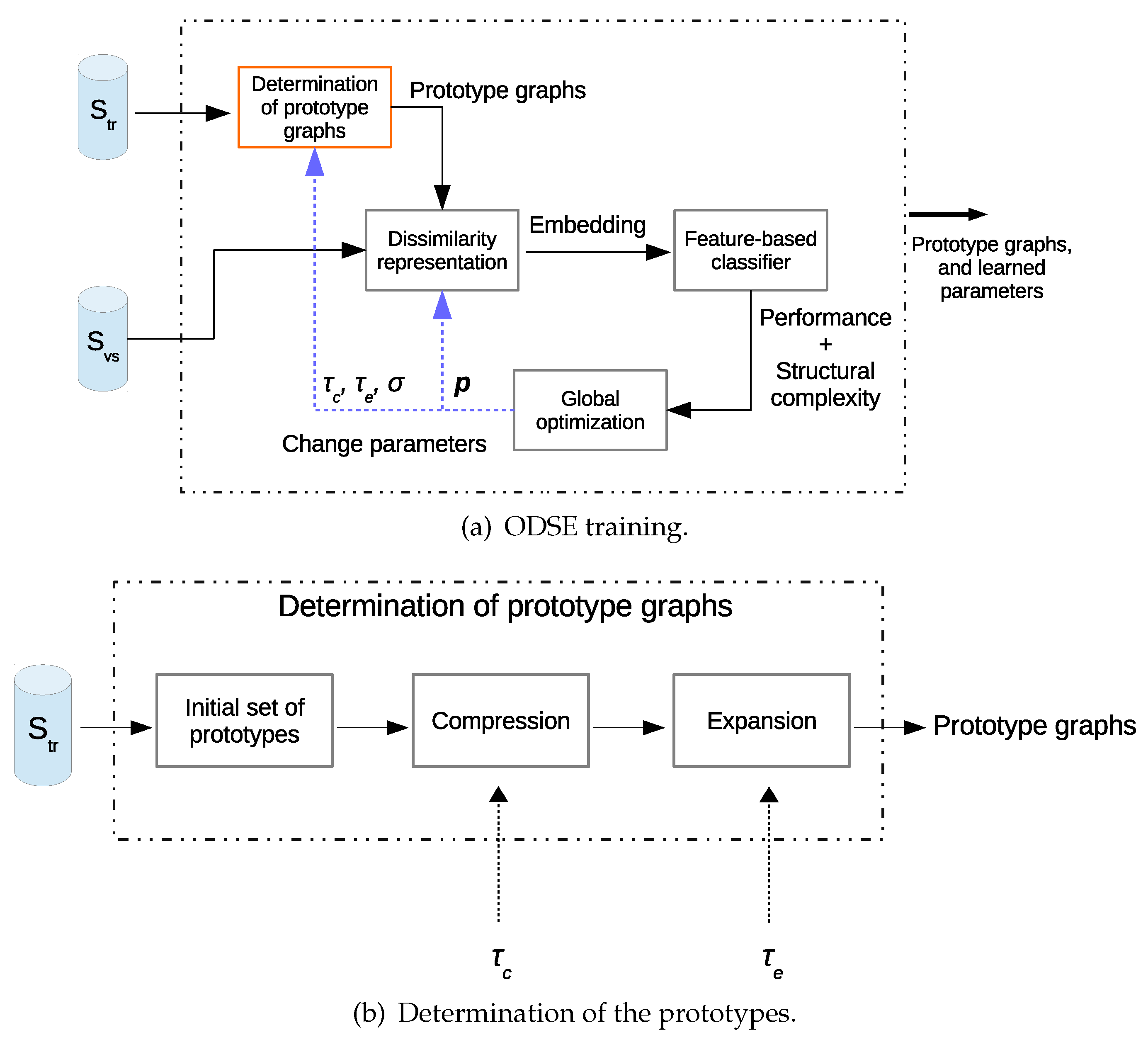
Figure 1a,b gives, respectively, the schematics of the ODSE training and determination of the prototypes. The ODSE classification model is defined by the RS, ${\mathcal{R}}_i$, the TWEC parameters, $\mathbf{p}$, and the model of the trained feature-based classifier. During the synthesis stage additional parameters are optimized: the kernel size $\sigma$ used by the entropy estimator and two thresholds, ${\tau }_c,{\tau }_e$, which are used in the compression and expansion operations, respectively. The ODSE model is synthesized by cross-validating the learned models on the training set ${\mathcal{S}}_{tr}$ over a validation set ${\mathcal{S}}_{vs}$. The global optimization is governed by a genetic algorithm, since the classification accuracy is used as part of the final objective and its analytical definition with respect to (w.r.t.) the model parameters is not available in closed form. A genetic algorithm, although it does not assure convergence towards a global optimum, is easily and effectively parallelizable, allowing to make use of multicore hardware/software implementations during the training stage.

3.1. The ODSE Objective Function

All parameters of the ODES model are arranged into codes, ${\underline{\mathbf{c}}}_i\in \mathcal{C}$. These include the two entropy thresholds ${\{{\tau }_c,{\tau }_e\}}_i$, the kernel size of the entropy estimator, ${\left\{\sigma \right\}}_i$, the weights of TWEC and any parameter of the vertex/edge label dissimilarity measures, all ranging in $[0,1]$. Since each ${\underline{\mathbf{c}}}_i$ induces a specific RS, ${\mathcal{R}}_i$, the optimization problem that characterizes the ODSE synthesis consists in deriving the best-performing RS:

$${\displaystyle \widehat{\mathcal{R}}=\underset{{\underline{\mathbf{c}}}_i\in \mathcal{C}}{\arg \max }f({\mathcal{S}}_{tr},{\mathcal{S}}_{vs},{\mathcal{R}}_i).}$$

(10)

The objective function (10) is defined as a linear convex combination of two objectives,

$$\begin{array}{c}\hfill f({\mathcal{S}}_{tr},{\mathcal{S}}_{vs},{\mathcal{R}}_i)=\eta f_1({\mathsf{\Phi }}^{{\mathcal{R}}_i}\left({\mathcal{S}}_{tr}\right),{\mathsf{\Phi }}^{{\mathcal{R}}_i}\left({\mathcal{S}}_{vs}\right))+(1-\eta )f_2({\mathsf{\Phi }}^{{\mathcal{R}}_i}\left({\mathcal{S}}_{tr}\right)),\end{array}$$

(11)

where $\eta \in [0,1]$ and ${\mathsf{\Phi }}^{{\mathcal{R}}_i}(·)$ shortens the dissimilarity representation of an entire dataset using the compressed-and-expanded RS instance, ${\mathcal{R}}_i$. The function $f_1(·,·)$ evaluates the recognition rate achieved on a validation set ${\mathcal{S}}_{vs}$, while $f_2(·)$ accounts for the quality of the synthesized classification model. Specifically,

$$f_2({\mathsf{\Phi }}^{{\mathcal{R}}_i}\left({\mathcal{S}}_{tr}\right))=\varsigma \mathrm{\Theta }+(1-\varsigma )\mathrm{{\rm Y}},$$

(12)

where $\varsigma \in [0,1]$, and $\mathrm{\Theta }$ denotes the cost related to the number $d_i$ of prototypes. Accordingly,

$$\mathrm{\Theta }=1-\frac{d_i-\zeta }{|{\mathcal{S}}_{tr}|},$$

(13)

where $\zeta$ is the number of classes characterizing the classification problem at hand. The second term, namely $\mathsf{{\rm Y}}$, captures the informativeness of the DM:

$$\mathsf{{\rm Y}}={\tilde{H}}_2\left({\underline{\mathbf{D}}}_n\right).$$

(14)

We consider the entropy factor (14) in the ODSE objective function (11) to increase the spread–dispersion of the DVs, which in turn is assumed to magnify the separability of the classes.

3.2. The ODSE Compression Operation

The compression operation searches for subsets of the initial RS, $\mathcal{R}$, which convey “similar information”; the initial RS is equal to the whole ${\mathcal{S}}_{tr}$ in the original ODSE. In order to describe the mechanism behind the ODSE compression operation, we need to define when a given subset $\mathcal{B}\subseteq \mathcal{R}$ of prototypes is compressible. Let ${\mathbf{D}}^{n\times d}$ be the DM corresponding to ${\mathcal{S}}_{tr}$ and $\mathcal{R}$, with $n=|{\mathcal{S}}_{tr}|$ and $d=\left|\mathcal{R}\right|$. Basically, $\mathcal{B}$ individuates a subset of $k=\left|\mathcal{B}\right|\le d$ columns of $\mathbf{D}$. Let $\mathbf{D}{\left[\mathcal{B}\right]}^{n\times k}$ be the filtered DM, i.e., the submatrix considering the prototypes in $\mathcal{B}$ only. We say that $\mathbf{D}{\left[\mathcal{B}\right]}^{n\times k}$ is compressible if

$${\tilde{H}}_2\left({\underline{\mathbf{D}}}_k\right)\le {\tau }_c,$$

(15)

where $0\le {\tau }_c\le 1$ is the compression threshold, and $\tilde{H}(·)$ estimates the QRE of the underlying joint distribution of $\mathbf{D}{\left[\mathcal{B}\right]}^{n\times k}$. In practice, the values of $\mathbf{D}{\left[\mathcal{B}\right]}^{n\times k}$ are interpreted as k measurements of a n-dimensional random vector; ${\underline{\mathbf{D}}}_k$ is the corresponding notation that we use throughout the paper to denote a sample of k random measurements elaborated from the DM. If the measurements are concentrated around a single n-dimensional support point, the estimated joint entropy is close to zero. This fact allows us to use Equation (15) as a systematic compression rule, retaining only a single representative graph of $\mathcal{B}$.

The selection of the subsets ${\mathcal{B}}_i,i=1,2,...,p$, is the first important algorithmic issue to be addressed. In the original ODSE [11], the subset selection has been performed by means of a randomized algorithm. The computational complexity of this approach was $O\left(d^{3}n\right)$, which does not scale adequately as the input size grows.

3.3. The ODSE Expansion Operation

The expansion focuses on each single $R_j\in \overleftarrow{\mathcal{R}}$, by analyzing the corresponding columns of the compressed DM, ${\mathbf{D}}^{n\times d}$. By denoting with ${\underline{\mathbf{D}}}_n$ the sample containing the n DVs corresponding to the j-th column of $\mathbf{D}$, we say that $R_j$ is expandable if

$${\tilde{H}}_2\left({\underline{\mathbf{D}}}_n\right)\le {\tau }_e,$$

(16)

where $0\le {\tau }_e\le 1$ is the expansion threshold. Practically, the information provided by the prototype is low if the n unidimensional measurements are concentrated around a single real-valued number. In such a case, the estimated entropy would be low, approaching zero as the underlying distribution becomes degenerate. Examples of such prototypes are outliers and prototype graphs that are equal in the same measure to all other graphs. Once an expandable $R_j$ is individuated through (16), $R_j$ is substituted by extracting $\zeta$ new graphs elaborated from ${\mathcal{S}}_{tr}$. Notably, those new graphs are derived by searching for recurrent subgraphs in a suitable subset of the training graphs.

Although the idea of trying to extract new features by searching for (recurrent) subgraphs is interesting, it is also very expensive in terms of computational complexity.

4. The Improved ODSE Graph Classifier

The improved ODSE system [40] is designed with the primary goal of a significant computational speed-up. The first variant, which is presented in Section 4.1, considers a simple yet fast RS initialization strategy and a more advanced compression mechanism. The compression is grounded on a formal result discussed in Section 4.1.2. The second variant is presented in Section 4.2. This version includes a more elaborated initialization of the RS, while it is characterized by the same CBC operation. The expansion operation, in both cases, has been greatly simplified. Finally, in Section 4.3 we discuss an important fact related to the efficiency of the implemented CBC.

4.1. ODSE with Clustering-Based Compression Operation

4.1.1. Randomized Representation Set Initialization

The initial RS $\mathcal{R}$, that is, the RS used during the synthesis, is defined by sampling the ${\mathcal{S}}_{tr}$ according to a selection probability, p. The size of the initial RS is thus characterized by a binomial distribution, selecting in average $|{\mathcal{S}}_{tr}|p$ graphs, with variance $|{\mathcal{S}}_{tr}|p(1-p)$. Although such a selection criteria is linear in the training set size, it operates blindly and may also cause an unbalanced selection of the prototypes w.r.t. the prior class distributions. However, such a simple sampling scheme is mostly used when the available hardware cannot process the entire dataset at hand.

4.1.2. Compression by a Clustering-Based Subset Selection

The entropy measured by the QRE estimator (3) is used to determine the compressibility of a subset of prototypes, $\mathcal{B}$. Since the entropy estimation is directly related to the DVs between the graphs of $\mathcal{B}$, we design a subset selection strategy that aggregates the initial prototypes according to their distances in the DS. Such subsets are guaranteed to be compressible by definition, avoiding thus the computational burden involved in entropy estimation.

We make use of the well-known Basic Sequential Algorithmic Scheme (BSAS) clustering algorithm (see the pseudo-code in Algorithm 1) with the aim of grouping the n-dimensional dissimilarity column-vectors ${\underline{\mathbf{x}}}_j,j=1,2,...,d$, with (hyper)spheres and using the Euclidean metric $d_2(·,·)$. The main reason behind the use of such a simple cluster generation rule is that it is much faster than other more sophisticated approaches [44], and it gives full control on the generated cluster geometry through a single real-valued parameter, $\theta \ge 0$. Since $\theta$ constrains each cluster ${\mathcal{B}}_l$ to have a maximum intra-cluster DV (i.e., a diameter) lower or equal to $2\theta$, we can deduce analytically the value of $\theta$ considering the particular instance of the kernel size ${\sigma }_c$ and entropy threshold ${\tau }_c$ used in Equation (15). Accordingly, the following theorem (see [40] for the proof) allows us to determine a partition $P(\theta ;{\tau }_c,{\sigma }_c)$ that contains clusters that are compressible by construction.

Algorithm 1 BSAS Cluster Generation Rule

Input: The ordered n input elements, a dissimilarity measure $d(·,·)$, the cluster radius $\theta$, and the maximum number of allowed clusters Q Output: The partition $P\left(\theta \right)$ 1: for $i=1,2,...,n$ do 2:  if $P\left(\theta \right)=\varnothing$ then 3:   Create a new cluster in $P\left(\theta \right)$ and define $x_i$ as the set representative 4:  else 5:   Get the distance value D from the closest representative modeling a cluster of the current partition $P\left(\theta \right)$ 6:   ${\displaystyle D=\underset{{\mu }_j\in P\left(\theta \right)}{\min }d(x_i,{\mu }_j)}$ 7:   if $D>\theta$ AND $\left|P\right(\theta \left)\right|<Q$ then 8:    Add a new cluster in $P\left(\theta \right)$ and define $x_i$ as the representative 9:   else 10:    Add $x_i$ in the j-th cluster and update the representative element 11:   end if 12:  end if 13: end for

Theorem 1.

The compressible partition $P(\theta ;{\tau }_c,{\sigma }_c)$ obtained on a training set ${\mathcal{S}}_{tr}$ of n graphs, is derived setting:

$$\theta \le \sqrt{\frac{{\tau }_{c}n{\sigma }_c^2\ln \left(2\right)}{2}}.$$

(17)

The optimization of ${\tau }_c$ and ${\sigma }_c$, together with the proof of Theorem 1, allows us to search for the best level of training set compression for the problem at hand. Algorithm 2 shows the pseudo-code of the herein described compression operation. Since the ultimate aim of the compression is to aggregate prototypes that convey similar information w.r.t. ${\mathcal{S}}_{tr}$, we represent a cluster using the minimum sum of distances (MinSOD) technique [45]. In fact, the MinSOD allows to select a single representative element $x_k\in {\mathcal{B}}_k$ according to the following expression:

$$x_k=\underset{x_j\in {\mathcal{B}}_k}{\arg \min }\sum _{x_i\in {\mathcal{B}}_k}{d}_2(x_j,x_i).$$

(18)

Eventually, the p prototype graphs, $B_i,i=1,2,...,p$, corresponding to the p computed MinSOD elements in the DS, populate the compressed RS, $\overleftarrow{\mathcal{R}}=\{B_1,B_2,...,B_p\}$.

Algorithm 2 Clustering-Based Compression Algorithm

Input: The initial set of prototype graphs $\mathcal{R},\left|\mathcal{R}\right|=d$, the DM ${\mathbf{D}}^{n\times d}$, the compression threshold ${\tau }_c$, and the kernel size ${\sigma }_c$ Output: The compressed set of prototype graphs $\overleftarrow{\mathcal{R}}$ 1: Configure BSAS setting $Q=\left|\mathcal{R}\right|$ and $\theta$ according to Equation (17) 2: Let $\mathcal{X}=({\underline{\mathbf{x}}}_1,{\underline{\mathbf{x}}}_2,...,{\underline{\mathbf{x}}}_d)$ be the (ordered) set of dissimilarity vectors elaborated from the columns of $\mathbf{D}$ 3: Execute the BSAS on $\mathcal{X}$. Let $P(\theta ;{\tau }_c,{\sigma }_c)=\{{\mathcal{B}}_1,{\mathcal{B}}_2,...,{\mathcal{B}}_p\}$ be the obtained compressible partition 4: Compute the MinSOD element ${\underline{\mathbf{b}}}_i$ of each cluster ${\mathcal{B}}_i,i=1,2,...,p$, according to Equation (18). Retrieve from $\mathcal{R}$ the prototype graph $B_i$ corresponding to each dissimilarity vector ${\underline{\mathbf{b}}}_i$ 5: Define $\overleftarrow{\mathcal{R}}={\bigcup }_{i=1}^p{B}_i$ 6: return $\overleftarrow{\mathcal{R}}$

The search interval for the kernel size ${\sigma }_c$ can be effectively reduced as follows:

$$0\le {\sigma }_c\le \sqrt{\frac{8}{\ln \left(2\right)}}.$$

(19)

A proof for (19) can be found in [40]. This bound is important, since it allows to narrow down the search interval for the kernel size ${\sigma }_c$, which is theoretically defined in the entire extended real line.

4.1.3. Expansion Based on Replacement with Maximum Dissimilar Graphs

The genetic algorithm evolves a population of models over iterations $t=1,2,...,\max$. Let ${\mathcal{R}}^0$ be defined as shown in Section 4.1.1, and let ${\mathcal{N}}^t={\mathcal{S}}_{tr}\setminus {\mathcal{R}}^{t-1}$ be the set of unselected training graphs at iteration $t\ge 1$. Finally, let ${\overleftarrow{\mathcal{R}}}^t$ be the compressed RS at iteration t. The herein described expansion operation makes use of the elements of ${\mathcal{N}}^t$ replacing in ${\overleftarrow{\mathcal{R}}}^t$ those prototypes that do not discriminate the classes. The expansion of a single prototype graph is still performed by the same criterion described in Section 3.3. Notably, if the estimated entropy of the j-th column vector is lower than the expansion threshold ${\tau }_e$, then l new training graphs are selected from ${\mathcal{N}}^t$ for each class, where $l\ge 1$. $\zeta \times l$ new graphs are selected such that they result maximally dissimilar w.r.t. the j-th prototype under analysis. The new expansion procedure is outlined in Algorithm 2 of [40].

Since compression and expansion are evaluated considering two different interpretations of the DM, we accordingly use two different kernel sizes: ${\sigma }_c$ and ${\sigma }_e$.

4.1.4. Analysis of Computational Complexity

The computational complexity is dictated by the execution of the genetic algorithm, $O(I+EP\times F)$. I is the cost of the RS initialization, E is the number of (maximum) evolutions, P is the population size, and finally F is the cost related to a single fitness function evaluation. Here, the initialization is linear in the training set size, $O\left(I\right)=O\left(\right|{\mathcal{S}}_{tr}\left|\right)$; in average we select $d^{\prime }=\lfloor |{\mathcal{S}}_{tr}|p\rfloor$ prototypes. The detailed cost related to the fitness function, $O\left(F\right)$, is articulated as the sum of the following costs:

$$\begin{array}{cc}\hfill O\left(F_1\right)& =O\left(n{d}^{\prime }g\right);O\left(F_2\right)=O\left(nQCe\right);\hfill \\ \hfill O\left(F_3\right)& =O\left(\overleftarrow{d}{n}^2\times \left(N\log \left(N\right)+\zeta l\right)\right);\hfill \\ \hfill O\left(F_4\right)& =O\left(n\overline{d}\right);O\left(F_5\right)=O\left(v\times \left(\overline{d}+kn\right)\right);\hfill \\ \hfill O\left(F_6\right)& =O\left(n^2\overline{d}\right).\hfill \end{array}$$

(20)

The first cost, $F_1$, is related to the computation of the initial DM corresponding to ${\mathcal{S}}_{tr}$ with RS obtained through the initialization of Section 4.1.1; g is the computational cost associated with the adopted IGM procedure. $F_2$ is related to the compression operation which consists of a single BSAS execution, where $C=d^{\prime }$ is the cache size of the MinSOD [45], $Q=d^{\prime }$, and $e=n$ is the cost of a single Euclidean distance computation. $F_3$ is the cost characterizing the expansion operation; N is the cardinality of the set ${\mathcal{N}}^t$. This operation is repeated at most $\overleftarrow{d}=|\overleftarrow{\mathcal{R}}|$ times, with a quadratic entropy estimation cost in the training set size. $F_4$ is the cost related to the embedding of the DM, and $F_5$ is due to the classification of the validation set using a k-NN rule based classifier—this cost is updated according to the specific classifier. $F_6$ is the cost for the QRE over the compressed and expanded DM.

As it is possible to deduce from Equation (20), the model synthesis is now characterized by a quadratic cost in the training set size, n, as well as in the RS size, d, while in the original ODSE it was (pseudo) cubic in both n and d.

4.2. ODSE with Mode Seeking Initialization

The ODSE variant described in this section does not include any expansion operation. The RS initialization is now part of the synthesis, since it depends on some of the parameters tuned during the optimization. Compression is still implemented as described in Section 4.1.2.

The initialization makes use of the Mode Seek (MS) algorithm [37], which is a well-known procedure that is able to individuate the modes of a distribution. For each class $c_i,i=1,2,...,\zeta$, and considering a user-defined neighborhood size $s\ge 1$, the algorithm proceeds as illustrated in Algorithm 3 of [40]. The elements of $\mathcal{R}$ found in this way are the estimated modes of the class distribution; it is a supervised algorithm.

The cardinality of $\mathcal{R}$ depends on the choice of s: the larger is s, the smaller $\mathcal{R}$. This approach is very appropriate when elements of the same class are distributed in different and heterogeneous clusters: the cluster representatives are the modes individuated by the MS algorithm. Moreover, the MS algorithm can be useful to filter out outliers, since they are characterized by a low neighborhood density. The procedure depends on s, which directly influences the outcome of the initialization. Additionally, since a neighborhood is defined in the graph domain, MS is also dependent on the TWEC weights. For this reason, the initialization is now performed during the ODSE synthesis.

To limit the complexity of such an initialization, in the experiments we systematically assign small values to s, constraining the search in small neighborhoods. A possible side effect of this choice is that we can find an excessive number of prototypes/modes. This effect is however attenuated by the use of the compression Algorithm 2.

Analysis of Computational Complexity

The overall computational cost of the synthesis is now bounded by $O(EP\times F)$; see (21). The two main steps of the fitness function involve the execution of the MS algorithm followed by the compression algorithm. The $F_1$ cost refers to the MS algorithm. $|c_i|$ is the number of training data belonging to the i-th class. $F_2$ refers to the computation of the initial DM, constructed using ${\mathcal{S}}_{tr}$ and the $d^{\prime }\le \left|{\mathcal{S}}_{tr}\right|$ prototypes derived with MS. $F_3$ is the cost of the compression operation, with $Q=d^{\prime }$. $F_4$, $F_5$, and $F_6$ are equivalent to the ones described in Section 4.2. The overall cost is dominated by the initialization stage (the $F_1$ cost), which is (pseudo) quadratic in the class size $|c_i|$, and quadratic in the neighborhood size, s,

$$\begin{array}{cc}\hfill O\left(F_1\right)& =O\left(n+\zeta |c_i|\times \left(|c_i|g+|c_i\left|\log \right(|c_i\left|\right)+s+s^2\right)\right);\hfill \\ \hfill O\left(F_2\right)& =O\left(n{d}^{\prime }g\right);O\left(F_3\right)=O\left(nQCe\right);\hfill \\ \hfill O\left(F_4\right)& =O\left(n\overline{d}\right);O\left(F_5\right)=O\left(v\times \left(\overline{d}+kn\right)\right);\hfill \\ \hfill O\left(F_6\right)& =O\left(n^2\overline{d}\right).\hfill \end{array}$$

(21)

4.3. The Efficiency of the ODSE Clustering-Based Compression

The BSAS (see Algorithm 1) is characterized by a linear computational complexity. However, due to the sequential processing nature, the outcome is sensitive to the data presentation order. In the following, we study the effect caused by the ordering of the input over the effectiveness of the CBC, by calculating what we called ODSE compression efficiency factor.

Let $s=({\underline{\mathbf{x}}}_1,{\underline{\mathbf{x}}}_2,...,{\underline{\mathbf{x}}}_n)$ be the sequence of dissimilarity vectors describing the n prototypes in the DS, which are presented in input to Algorithm 1. Let $\mathsf{\Omega }\left(s\right)$ be the set of all permutations of the sequence s. We define the optimal compression ratio ${\rho }^{*}\left(s\right)$ for the sequence s as:

$${\rho }^{*}\left(s\right)=\underset{s_i\in \mathsf{\Omega }\left(s\right)}{\max }\rho \left(s_i\right)=\underset{s_i\in \mathsf{\Omega }\left(s\right)}{\max }\left|\mathcal{R}\right|/|{\overleftarrow{\mathcal{R}}}_i|,$$

(22)

where ${\overleftarrow{\mathcal{R}}}_i$ is the compressed RS obtained by analyzing the prototypes arranged according to $s_i$, and $\mathcal{R}$ is the uncompressed RS, i.e., the initial RS. Let $\widehat{\rho }\left(s\right)$ be the effective compression ratio, achieved by ODSE considering a generic ordering of s. The ratio

$$\xi =\underset{n\to \infty }{\lim }\widehat{\rho }\left(s\right)/{\rho }^{*}\left(s\right)\in [0,1],$$

(23)

describes the asymptotic efficiency of the ODSE compression as the initial RS size grows.

Theorem 2.

The asymptotic worst-case ODSE compression efficiency factor is $\xi =2/3$.

The proof can be found in Appendix A. An interpretation of the result of Theorem 2 is that the asymptotic efficiency of the implemented CBC varies within the $[2/3,1]$ range of the optimum compression.

5. ODSE with the MST-Based Rényi Entropy Estimator

In the following, we contextualize the MST-RE estimation technique introduced in Section 2.2 as a component of the improved ODSE system presented in Section 4. Notably, we discuss a theorem for determining the $\theta$ parameter used in the compression operation (Algorithm 2). In this case, we generate clusters according to the particular instance of ${\tau }_c$ and of the $\gamma$ parameter, since the kernel size parameter, ${\sigma }_c$, is not present in the MST-based estimator. The $\gamma$ parameter is optimized during the ODSE synthesis. While $\gamma$ is defined in $(0,d)$, where d is the dimensionality of the samples, we restrict the search interval to $(0,U]$, with $U=3$ in the experiments. This technical choice is motivated by the fact that $\gamma$ is used in Equation (5) as exponent, and an excessively large value would easily cause overflow problems for the floating-point representation of the MST length variable.

Theorem 3.

Considering the instances of γ and ${\tau }_c$, a compressible partition $P(\theta ;{\tau }_c,\gamma )$ is derived executing the BSAS algorithm on $n=|{\mathcal{S}}_{tr}|$ training graphs by setting:

$$\theta \le 2^{{\tau }_c-1}{n}^{\frac{{\tau }_c}{2}}{\beta }^{\frac{-{\tau }_c+1}{\gamma }}c\left(\gamma \right),\mathrm{where}0\le c\left(\gamma \right)\le 2^{\frac{\alpha }{\gamma }}.$$

(24)

The proof of this theorem can be found in Appendix B. Defining $\theta$ according to Equation (24) constrains the BSAS to generate clusters that are compressible by construction. Since ${\tau }_c$ and $\gamma$ are optimized during the ODSE synthesis, the result of Theorem 3, likewise the one of Theorem 1, allows us to evaluate different levels of training set compression according to the overall system performance. It goes without saying that computational complexity discussed in the previous sections is readily updated by considering the cost of the MST-based estimator (see Equation (9) for details).

6. Experimental Section

In Section 6.1 we introduce the IAM benchmarking datasets considered in our study; in Section 6.2 we present the experimental setting. Finally, in Section 6.3 we show and discuss the results.

6.1. Datasets

The experimental evaluation is performed on the well-known IAM graph benchmarking database [46]. The IAM database contains several datasets representing real-world data: from images to biochemical compounds. In particular, we use the Letter LOW (L-L), Letter MED (L-M), Letter HIGH (L-H), AIDS (AIDS), Proteins (P), GREC (G), Mutagenicity (M), and finally the Coil-Del (C-D) datasets. The first three datasets denote digitized characters modeled as labeled graphs, which are characterized by three different levels of noise. The AIDS, P, and M datasets represent biochemical networks, while G and C-D are images of various type. For the sake of brevity, we report only essential details in

Table 2. IAM datasets. See [46] for details. “#” indicates cardinality of the sets.

DS	# (tr, vs, ts)	Classes	Average $\left|\mathcal{V}\right|$	Average $\left|\mathcal{E}\right|$
L-L	(750, 750, 750)	15	4.7	3.1
L-M	(750, 750, 750)	15	4.7	3.2
L-H	(750, 750, 750)	15	4.7	4.5
AIDS	(250, 250, 1500)	2	15.7	16.2
P	(200, 200, 200)	6	32.6	62.1
G	(286, 286, 528)	22	11.5	12.2
M	(1500, 500, 2337)	2	30.3	30.8
C-D	(2400, 500, 1000)	100	21.5	54.2

, referring the reader to [46] (and references therein) for a more in-depth discussion about the data. Moreover, since each dataset contains graphs characterized by different vertex and edge labels, we adopted the same vertex and edge dissimilarity measures described in [11,12].

6.2. Experimental Setting

The ODSE system version described in Section 4.1 is denoted as ODSE2v1, while the version described in Section 4.2 as ODSE2v2. These two versions make use of the QRE estimator; the setting of the clustering algorithm parameter $\theta$ used during the compression is hence performed according to the result of Theorem 1. By following the same algorithmic scheme, we consider two additional ODSE variants adopting the MST-RE estimator. We denote these two variants as ODSE2v1-MST and ODSE2v2-MST. $\theta$ is hence determined according to the proof of Theorem 3. However, the MST-based estimator is conceived for high-dimensional data. As a consequence, in the ODSE2v1-MST system version we still use the QRE estimator in the expansion operation. We adopted two feature-based classifiers operating in the DS. The first one is a k-nearest neighbors (k-NN) rule based classifier equipped with the Euclidean distance, testing three values of k: 1, 3, and 5. We also consider a fast MMN, which is trained with the ARC algorithm [43]. The four aforementioned ODSE variants (i.e., ODSE2v1, ODSEv2, ODSEv1-MST, and ODSE2v2-MST) are therefore replicated into additional four variants that are straightforwardly denoted as ODSE2v1-MMN, ODSEv2-MMN, ODSEv1-MST-MMN, and ODSE2v2-MST-MMN, meaning that we just use the neuro-fuzzy MMN on the embedding space, instead of the k-NN.

Table 3. Summary of the ODSE configurations evaluated in the experiments. The “Init” column refers to the RS initialization scheme, “Compression/Est.” refers to the compression algorithm and adopted entropy estimator, “Expansion/Est.” the same but for the expansion algorithm, and “Obj. Func. (14)” refers to the entropy estimator adopted in Equation (14). Finally, “FB Class.” specifies the feature-based classifier operating in the DS.

Acronym	Init	Compression/Est.	Expansion/Est.	Obj. Func. (14)	FB Class.
ODSE2v1	Section 4.1.1	Section 4.1.2/QRE	Section 4.1.3/QRE	QRE	k-NN
ODSE2v2	Section 4.2	Section 4.1.2/QRE	–	QRE	k-NN
ODSE2v1-MST	Section 4.1.1	Section 4.1.2/MST-RE	Section 4.1.3/QRE	MST-RE	k-NN
ODSE2v2-MST	Section 4.2	Section 4.1.2/MST-RE	–	MST-RE	k-NN
ODSE2v1-MMN	Section 4.1.1	Section 4.1.2/QRE	Section 4.1.3/QRE	QRE	MMN
ODSE2v2-MMN	Section 4.2	Section 4.1.2/QRE	–	QRE	MMN
ODSE2v1-MST-MMN	Section 4.1.1	Section 4.1.2/MST-RE	Section 4.1.3/QRE	MST-RE	MMN
ODSE2v2-MST-MMN	Section 4.2	Section 4.1.2/MST-RE	–	MST-RE	MMN

summarizes all ODSE configurations evaluated in this paper.

Experiments are executed with a (fixed) population size of 30 individuals, and performing a maximum of 40 evolutions; a check on the fitness value is however performed terminating the optimization if the fitness does not change for 15 consecutive evolutions. This choice allows for a fair comparison with the previously obtained results in [11,40]. The genetic algorithm performs roulette wheel selection, two-point crossover, and random mutation on the aforementioned codes ${\underline{\mathbf{c}}}_i$, encoding the real-valued model parameters; in addition, the genetic algorithm implements an elitism strategy which automatically imports the fittest individual into the next population. In all configurations, we executed the system setting $\eta =0.9$ and $\varsigma =0.2$ in Equations (11) and (12), respectively. Moreover, the s parameter affecting the MS algorithm has been set as follows: 10 for the L-L, L-M, and L-H, 20 for AIDS, 2 for P, 8 for G, and finally 100 for either M and C-D. Note that these values have been defined according to the training dataset size and considering some preliminary fine tuning. Each dataset has been processed five times using different random seeds, reporting hence the average test set classification accuracy together with its standard deviation. We show also the required average serial CPU time and the average RS size obtained after the model synthesis. Tests have been conducted on a regular desktop machine with an Intel Core2 Quad CPU Q6600 at 2.40 GHz and 4 Gb of RAM; software is implemented in C++ on Ubuntu 14.04 using the SPARE library [47]. Finally, computing time is measured using the clock() routine of the standard ctime library.

6.3. Results and Discussion

All test set classification accuracy results have been collected in

Table 4. Test set classification accuracy results. Lines in grey denote novel results introduced in this paper. The “-” sign means that the result is not available to our knowledge. Bold values denote significant differences as discussed in the text.

Classifier	Dataset								Rank
	L-L	L-M	L-H	AIDS	P	G	M	C-D
Reference systems
RPS + TWEC + k-NN, $k=1$	98.4	96.0	95.0	98.5	45.5	95.0	69.0	81.0	15
k-NN + TWEC, $k=1$	96.8	66.3	36.3	73.9	52.1	95.0	57.7	61.2	38
RPS+TWEC + k-NN, $k=3$	98.6	97.2	94.7	98.2	40.5	92.0	68.7	63.2	23
k-NN + TWEC, $k=3$	97.5	57.4	39.1	71.4	48.5	91.8	56.1	33.7	39
RPS+TWEC + k-NN, $k=5$	98.3	97.1	95.0	97.6	35.4	84.8	68.5	59.7	32
k-NN + TWEC, $k=5$	97.6	60.4	42.2	76.7	43.0	88.5	56.9	27.8	40
RPS + TWEC + MMN	98.0	96.0	93.6	97.4	49.5	95.0	66.0	68.4	28
SOA systems
GMM + soft all + SVM [26]	99.7	93.0	87.8	-	-	99.0	-	98.1	12
Fuzzy k-means+soft all + SVM [26]	99.8	98.8	85.0	-	-	98.1	-	97.3	9
sk + SVM [48]	99.7	85.9	79.1	97.4	-	94.4	55.4	-	30
le + SVM [48]	99.3	95.9	92.5	98.3	-	96.8	74.3	-	7
PCA + SVM [49]	92.7	81.1	73.3	98.2	-	92.9	75.9	93.6	26
MDA + SVM [49]	89.8	68.5	60.5	95.4	-	91.8	62.4	88.2	37
svm + SVM [50]	99.2	94.7	92.8	98.1	71.5	92.2	68.3	-	17
svm + kPCA [50]	99.2	94.7	90.3	98.1	67.5	91.6	71.2	-	14
lgq [51]	81.5	-	-	-	-	86.2	-	-	35
bayes1 [52]	80.4	-	-	-	-	80.3	-	-	36
bayes2 [52]	81.3	-	-	-	-	89.9	-	-	34
FMGE + k-NN [30]	97.1	75.7	66.5	-	-	97.5	69.1	-	31
FMGE + SVM [30]	98.2	83.1	70.0	-	-	99.4	76.5	-	21
d-sps-SVM [31]	99.5	95.4	93.4	98.2	73.0	92.5	71.5	-	8
GRALGv1 [12]	98.2	75.6	69.6	99.7	-	97.7	73.0	94.0	10
GRALGv2 [12]	97.6	89.6	82.6	99.7	64.6	97.6	73.0	97.8	6
Original ODSE
ODSE, $k=1$ [11]	98.6	96.8	96.2	99.6	61.0	96.2	73.4	-	1
Improved ODSE with QRE
ODSE2v1, $k=1$ [40]	99.0	97.0	96.1	99.1	61.2	98.1	68.2	78.1	4
ODSE2v2, $k=1$ [40]	98.7	97.1	95.4	99.5	51.9	95.4	68.1	77.2	5
ODSE2v1, $k=3$ [40]	99.0	97.2	96.1	99.3	41.4	90.2	68.7	64.3	13
ODSE2v2, $k=3$ [40]	98.8	97.4	95.1	99.4	31.4	38.0	69.4	59.0	24
ODSE2v1, $k=5$ [40]	99.1	96.8	95.2	99.0	38.9	85.4	69.0	58.6	27
ODSE2v2, $k=5$ [40]	98.7	97.0	95.6	99.4	31.3	82.5	70.0	54.0	25
ODSE2v1-MMN	98.3	95.2	94.0	99.3	53.1	94.5	67.9	62.8	22
ODSE2v2-MMN	97.8	95.6	93.6	99.6	48.7	94.8	68.2	59.2	29
Improved ODSE with MST-RE
ODSE2v1-MST, $k=1$	98.6	96.8	98.9	99.3	61.3	95.6	70.0	81.0	3
ODSE2v2-MST, $k=1$	98.4	97.1	96.0	99.7	51.0	94.1	71.6	82.0	2
ODSE2v1-MST, $k=3$	98.7	97.0	96.8	99.5	43.0	92.3	68.6	64.8	11
ODSE2v2-MST, $k=3$	98.8	96.9	96.0	99.7	35.0	91.0	69.4	60.0	16
ODSE2v1-MST, $k=5$	99.0	96.8	95.6	99.6	41.4	85.0	68.6	60.0	18
ODSE2v2-MST, $k=5$	98.8	97.0	95.5	99.7	32.9	83.3	70.0	54.0	19
ODSE2v1-MST-MMN	97.9	95.4	93.6	99.3	49.9	95.0	68.3	62.6	20
ODSE2v2-MST-MMN	97.9	95.1	91.8	99.2	48.5	94.8	67.1	59.0	33

, including those of three baseline reference systems and several state-of-the-art (SOA) classification systems based on graph embedding techniques. The table is divided in appropriate macro blocks to improve readability. The three reference systems are denoted as RPS + TWEC + k-NN, k-NN + TWEC, and RPS + TWEC + MMN. The first one performs a (class-independent) randomized selection of the training graphs to develop the dissimilarity representation of the input data. This system adopts the same TWEC used in ODSE and performs the classification in the DS by means of a k-NN classifier equipped with the Euclidean distance. The second one differs from the first system by instead using the MMN. Finally, the third reference system operates directly in $\mathcal{G}$ by means of a k-NN rule based classifier equipped with TWEC. In all cases, to obtain a fair comparison, the configuration of the dissimilarity measures for the vertex/edge labels is consistent with the one adopted previously. Additionally, $k=1,3$, and 5 are used in the k-NN rule, performing the TWEC parameters optimization (i.e., the weights in $[0,1]$) by means of the same aforementioned genetic algorithm implementation. Therefore, also in this case, the test set results must be intended as average of five different runs (however we omit standard deviations for the sake of brevity).

Table 4 presents the obtained test set classification accuracy results, while

Table 5. Standard deviations of ODSE results shown in Table 4. (Lines in grey denote novel results introduced in this paper).

Classifier	Dataset
	L-L	L-M	L-H	AIDS	P	G	M	C-D
ODSE [11]	0.0256	1.2346	0.2423	0.0000	0.7356	0.4136	0.6586	-
ODSE2v1, $k=1$ [40]	0.0769	0.2309	0.1539	0.0000	2.6242	1.3350	0.5187	4.3863
ODSE2v2, $k=1$ [40]	0.0769	0.0769	0.4000	0.0000	0.2915	0.8021	0.5622	2.2654
ODSE2v1, $k=3$ [40]	0.0769	0.2309	0.2666	0.0000	1.0513	1.2236	0.0856	0.0577
ODSE2v2, $k=3$ [40]	0.0769	0.4618	5.0800	0.1924	1.1666	3.1540	0.0356	1.2361
ODSE2v1, $k=5$ [40]	0.5047	0.0769	0.9365	0.1924	0.5050	2.5585	0.3803	1.3279
ODSE2v2, $k=5$ [40]	0.1333	0.2309	0.0769	0.0000	2.7815	4.5220	1.2666	0.0026
ODSE2v1-MMN	0.1520	0.3320	0.3932	0.1861	1.7740	0.7315	1.1300	1.0001
ODSE2v2-MMN	0.2022	0.2022	0.7682	0.0000	2.7290	1.3584	1.4080	0.3896
ODSE2v1-MST, $k=1$	0.0730	0.0730	0.1115	0.2772	1.5500	0.1055	1.0786	0.4163
ODSE2v2-MST, $k=1$	0.0596	0.2231	0.0730	0.0000	1.1660	0.2943	0.9534	0.2146
ODSE2v1-MST, $k=3$	0.1192	0.1520	0.0942	0.6982	1.0940	0.0000	0.5926	1.7088
ODSE2v2-MST, $k=3$	0.1460	0.2022	0.0730	0.0000	0.0000	0.1112	0.2365	0.5655
ODSE2v1-MST, $k=5$	0.1115	0.0942	0.2190	0.0596	0.4748	0.0000	0.0547	1.2356
ODSE2v2-MST, $k=5$	0.0730	0.0596	0.9933	0.0000	0.0000	0.1112	1.0023	0.9563
ODSE2v1-MST-MMN	0.1115	0.4216	0.7624	0.3217	2.5735	0.3067	0.7926	0.9899
ODSE2v2-MST-MMN	0.0596	0.7636	0.7477	0.0000	2.7290	0.5828	0.8911	1.2020

gives the corresponding standard deviations. We provide two types of statistical evaluation of such results. First, we perform pairwise comparisons by means of the t-test; we adopt the usual 5% as significance threshold. Notably, we check if any of the improved ODSE variants significantly outperforms, for each single dataset, both the reference systems and original ODSE. Best results satisfying such a condition are reported in bold in Table 4. In addition to the pairwise comparisons, we calculate also a global ranking of all classifiers by means of the Friedman’s test. Missing values are replaced by the dataset-specific averages.

First of all, we note that results obtained with the baseline reference systems are always worse than those obtained with ODSE. Test set classification accuracy percentages obtained by ODSE2v1-MST and ODSE2v2-MST are comparable with those of ODSE2v1 and ODSE2v2, although we note a slightly general improvement for the first two variants. Results are also more stable varying the neighborhood size parameter, k, of the k-NN rule. It is worth noting that, for difficult datasets such as P and C-D, increasing the neighborhood size in the k-NN rule significantly affects the test set performance (i.e., results degrade considerably). Test set results obtained by means of the MMN operating in the DS are in general (slightly) inferior w.r.t. the ones obtained with the k-NN rule with $k=1$. This result is not too unusual since the k-NN rule is a valuable classifier, especially in absence of noisy data. Since ODSE operates by searching for the best-performing DS for the data at hand, we may deduce that the embedding vectors are discriminative for the classes. Test set results on the first four datasets (i.e., L-L, L-M, L-H, and AIDS) denote an important improvement over a large part of the SOA systems. On the other hand, results over the P, G, and M datasets are comparable w.r.t. those of the SOA systems. For all ODSE configurations, we observe non convincing results on the C-D dataset; in this case results are comparable only with those of the reference systems (first block of Table 4). However, a rational reason explaining this fact is not yet emerged from the tests, requiring thus further investigations. The global picture provided by the “Rank” column shows that the ODSE classifiers rank very well w.r.t. the SOA systems. Standard deviations (Table 5) are reasonably small, denoting a reliable classifier regardless the particular ODSE variant.

We demonstrated that the asymptotic computational complexity of ODSE2 is quadratic, while for the original ODSE it was cubic. Here, in order to complement this result with experimental evidence, we discuss also the physical computing time. The calculated serial CPU time, for each dataset, is shown in

Table 6. Average serial CPU time in minutes (and speed-up factor w.r.t. the original ODSE system) considering ODSE model synthesis and test set evaluation. In the k-NN case, we report the results with $k=1$ only. (Lines in grey denote novel results introduced in this paper).

Classifier	Dataset
	L-L	L-M	L-H	AIDS	P	G	M	C-D
ODSE [11]	63274	52285	28938	394	8460	601	43060	-
ODSE2v1 [40]	284 (222)	329 (158)	328 (88)	38 (10)	3187 (3)	210 (3)	3494 (12)	2724
ODSE2v2 [40]	126 (502)	268 (195)	183 (158)	110 (3)	1683 (5)	96 (6)	10326 (4)	8444
ODSE2v1-MMN	129 (490)	284 (184)	263 (110)	17 (23)	3638 (2)	170 (4)	8837 (5)	5320
ODSE2v2-MMN	195 (324)	422 (124)	183 (158)	86 (5)	1444 (6)	77 (8)	28511 (2)	20301
ODSE2v1-MST	213 (297)	231 (226)	225 (129)	18 (22)	3860 (2)	168 (4)	2563 (17)	3261
ODSE2v2-MST	145 (463)	160 (327)	107 (270)	93 (4)	2075 (4)	74 (8)	7675 (6)	10092
ODSE2v1-MST-MMN	201 (315)	249 (210)	205 (141)	15 (26)	3450 (2)	155 (4)	5496 (8)	7135
ODSE2v2-MST-MMN	117 (541)	176 (292)	118 (245)	83 (5)	1380 (6)	75 (8)	28007 (2)	16599

, which includes both ODSE synthesis and test set evaluation. The ODSE variants based on the MST entropy estimator are faster, with the only exception for the P and C-D datasets. This fact is magnified on the first four datasets, in which the speed-up factor w.r.t. the original ODSE considerably increases. The speed-up factors obtained for the first three datasets are one order of magnitude higher than the ones obtained in the other datasets. In order to provide an explanation for such differences, we need to take a closer look at the dataset details shown in Table 2, computational complexity in Equations (20) and (21), and the computational complexity of the original ODSE [11]. It is possible to notice that the first three datasets contain smaller (in average) labeled graphs. Therefore, this suggests to look for the related terms in the computational complexity formulae. The g term (the cost of the graph matching algorithm) is directly affected by the size of the graphs and appears in $F_1$ Equation (20) and $F_1,F_2$ in Equation (21). The same g term appears also in $F_1$ of Equation 24 in [11]. In the original ODSE version [11], the dissimilarity matrix is constructed using an initial set of prototypes equal to the training set (then it is compressed and expanded). In the new version presented in this paper, we instead use a reduced set with $d^{\prime }$ elements. In the first variant that we presented, $d^{\prime }$ graphs are selected randomly from the training set based on a selection probability. In the second variant, instead, we use the MS algorithm, which finds a much lower number of representatives (although, as said in the experimental setting section, we use a conservative setting for MS). This fact provides a first rational justification for explaining the aforementioned differences. In fact, graph matching algorithms are expensive from the computational viewpoint (the adopted algorithm is quadratic in the number of vertices). In addition, compression and expansion operations are now much faster. As shown in

Table 7. Average cardinality of the best-performing RS. In the k-NN case, we report the results with $k=1$ only since results with $k=3$ and $k=5$ are similar. (Lines in grey denote novel results introduced in this paper).

Classifier	Dataset
	L-L	L-M	L-H	AIDS	P	G	M	C-D
ODSE [11]	435	750	750	250	200	283	1500	-
ODSE2v1 [40]	146	449	449	8	197	283	760	615
ODSE2v2 [40]	183	431	338	7	82	126	801	770
ODSE2v1-MM	136	192	144	6	190	163	563	555
ODSE2v2-MM	197	546	80	2	93	115	815	740
ODSE2v1-MST	597	595	597	6	198	283	687	618
ODSE2v2-MST	551	574	447	61	122	129	813	775
ODSE2v1-MST-MMN	600	606	500	5	190	184	424	549
ODSE2v2-MST-MMN	550	580	411	61	93	115	456	733

, the new ODSE versions compute a smaller RS; a direct consequence of the improved compression operation. This is another important factor contributing to the overall speed-up, since smaller RSs imply less graph matching computations during the validation and test stages; we remind that ODSE is trained by cross-validation. Clearly, there are also other factors, such as the convergence of the optimization algorithm, which might be affected by the specific dataset at hand.

As expected, the sped-up factors obtained by using the MMN as classifier are in general higher than those obtained with kNN. In fact, MMN synthesizes a classification model over embedded training data. This significantly reduces the computing time necessary for the evaluation of the test set (and also of the validation stage). This is demonstrated by the results in

Table 8. Average serial CPU time in seconds for test set evaluation only. For simplicity, we report the results of only one system variant operating in the DS with the k-NN classifier and only one with the MMN. (Lines in grey denote novel results introduced in this paper).

Classifier	Datasets
	L-L	L-M	L-H	AIDS	P	G	M	C-D
ODSE2v1-MST, $k=1$	0.740	0.740	0.740	0.130	0.020	0.060	9.020	9.700
ODSE2v1-MST-MMN	0.105	0.105	0.105	0.005	0.014	0.045	6.600	5.250

, where we report the CPU time for the test set evaluation only. This fact might assume more importance in particular applications, especially in those where the synthesis of the classifier can be effectively performed only once in off-line mode and the classification model is employed to process high-rate data streams in real-time [53].

Let us focus now on the structural complexity of the synthesized classification models. The cardinality of the best-performing RSs are shown in Table 6. It is possible to note that the cardinality are slightly bigger for those variants operating with MST-RE (especially in the first three datasets, i.e., L-L, L-M, and L-H). From this fact we deduce that, when configuring the CBC procedure with the MST-RE estimator, the ODSE classifier, in order to obtain good results in terms of test set accuracy, requires a more complex model w.r.t. the variants involving the QRE estimator. This behavior is, however, magnified by the setting of the objective function parameter $\eta$ adopted in our experiment, which biases the ODSE system towards maximizing the recognition rate. Notably, variants operating with the MMN develop considerable less costly classification models (see Table 7 and

Table 9. Average number of hyperboxes generated by the MMN. The number of hyperboxes can be used as a complexity indicator of the model synthesized by the MMN on the DS. Such values should be taken into account considering also the dataset characteristics of Table 2 and the average RS sizes in Table 7. (Lines in grey denote novel results introduced in this paper).

Classifier	Dataset
	L-L	L-M	L-H	AIDS	P	G	M	C-D
ODSE2v1-MMN	15	39	34	5	43	27	164	357
ODSE2v2-MMN	15	28	41	4	48	28	159	368
ODSE2v1-MST-MMN	15	27	38	3	48	28	168	348
ODSE2v2-MST-MMN	15	27	34	4	43	27	175	365

for the details). This particular aspect becomes very important in resource-constrained scenarios and/or when the input datasets are large. The considerable reductions of the RS size achieved here strengthen the fact that the entropy estimation operates adequately in the dissimilarity representation context.

7. Conclusions and Future Directions

In this paper, we have presented different variants of the improved ODSE graph classification system. All discussed variants are based on the characterization of the informativeness of DMs through the estimation of the $\alpha$-order Rényi entropy. The first adopted estimator computes the QRE by means of a kernel-based density estimator, while the second one uses the length of an entropic MST. The improved ODSE system has been designed by providing different strategies for the initialization, compression, as well as for the expansion operation of the RS. In particular, we conceived a fast CBC scheme, which allowed us to directly control the compression level of the data through the explicit setting of the cluster radius parameter. We provided formal proofs related to the two estimation techniques, which enabled us to determine the value of cluster radii analytically according to the ODSE model optimization procedure. We have studied also the asymptotic worst-case efficiency of the CBC scheme implemented by means of a sequential cluster generation rule (BSAS).

Experimental evaluations and comparisons with several state-of-the-art systems have been performed on well-known benchmarking datasets of labeled graphs (IAM database). We used two different feature-based classifiers operating in the DS: the k-NN classifier equipped with the Euclidean distance and a neurofuzzy MMN trained with the ARC algorithm. Overall, the variants adopting the MST-based estimator were faster but less parsimonious for what concerns the synthesized ODSE model (i.e., the cardinality of the best-performing RS was larger). The use of the k-NN rule (with $k=1$) produced slightly better test set accuracy results w.r.t. the MMN classifier, while in the latter case we observed important differences in term of (serial) CPU computing time, especially for what concerns the test set processing. The test set classification accuracy results confirmed the effectiveness of the ODSE classifier w.r.t. state-of-the-art standards. Moreover, the significative CPU time improvements w.r.t. the original ODSE version, and the highly parallelizable global optimization scheme based on genetic algorithms, bring the ODSE graph classifier one step closer towards the applicability to larger labeled graphs and big datasets.

The vector representation of the input graphs have been obtained directly using the rows of the DM. Such a choice, while it is known to be effective, has been mainly dictated by the computing time requirements of the system. It is worth analyzing the performance of ODSE also when the embedding space is obtained by a (non)linear embedding of the (corrected) pairwise dissimilarity values [54]. Future experiments include testing other core IGM procedures [55] and additional $\alpha$-order Rényi entropy estimators and feature-based classifiers.

References

- Livi, L.; Rizzi, A. The graph matching problem. Pattern Anal. Appl. 2013, 16, 253–283. [Google Scholar] [CrossRef]
- Dörfler, F.; Bullo, F. Kron Reduction of Graphs With Applications to Electrical Networks. IEEE Trans. Circuits Syst. 2013, 60, 150–163. [Google Scholar] [CrossRef]
- Porfiri, M.; Stilwell, D.J.; Bollt, E.M. Synchronization in random weighted directed networks. IEEE Trans. Circuits Syst. I Regul. Pap. 2008, 55, 3170–3177. [Google Scholar] [CrossRef]
- Livi, L.; Giuliani, A.; Rizzi, A. Toward a multilevel representation of protein molecules: Comparative approaches to the aggregation/folding propensity problem. Inf. Sci. 2016, 326, 134–145. [Google Scholar] [CrossRef]
- Di Paola, L.; De Ruvo, M.; Paci, P.; Santoni, D.; Giuliani, A. Protein contact networks: An emerging paradigm in chemistry. Chem. Rev. 2012, 113, 1598–1613. [Google Scholar] [CrossRef] [PubMed]
- Bianchi, F.M.; Livi, L.; Rizzi, A. Matching of Time-Varying Labeled Graphs. In Proceedings of the 2013 International Joint Conference on Neural Networks (IJCNN), Dallas, TX, USA, 4–9 August 2013; pp. 1–8. [Google Scholar]
- Serratosa, F.; Cortés, X.; Solé-Ribalta, A. Component retrieval based on a database of graphs for hand-written electronic-scheme digitalisation. Expert Syst. Appl. 2013, 40, 2493–2502. [Google Scholar] [CrossRef]
- Noma, A.; Graciano, A.B.V.; Cesar, R.M., Jr.; Consularo, L.A.; Bloch, I. Interactive image segmentation by matching attributed relational graphs. Pattern Recognit. 2012, 45, 1159–1179. [Google Scholar] [CrossRef]
- Chen, L. EM-type method for measuring graph dissimilarity. Int. J. Mach. Learn. Cybern. 2014, 5, 625–633. [Google Scholar] [CrossRef]
- Jothi, R.B.G.; Rani, S.M.M. Hybrid neural network for classification of graph structured data. Int. J. Mach. Learn. Cybern. 2015, 6, 465–474. [Google Scholar] [CrossRef]
- Livi, L.; Rizzi, A.; Sadeghian, A. Optimized dissimilarity space embedding for labeled graphs. Inf. Sci. 2014, 266, 47–64. [Google Scholar] [CrossRef]
- Bianchi, F.M.; Livi, L.; Rizzi, A.; Sadeghian, A. A Granular Computing approach to the design of optimized graph classification systems. Soft Comput. 2014, 18, 393–412. [Google Scholar] [CrossRef]
- Marfil, R.; Escolano, F.; Bandera, A. Graph-Based Representations in Pattern Recognition and Computational Intelligence. In Bio-Inspired Systems: Computational and Ambient Intelligence; Cabestany, J., Sandoval, F., Prieto, A., Corchado, J.M., Eds.; Springer: Berlin, Germany, 2009; Volume 5517, pp. 399–406. [Google Scholar]
- Bengoetxea, E.; Larrañaga, P.; Bloch, I.; Perchant, A.; Boeres, C. Inexact graph matching by means of estimation of distribution algorithms. Pattern Recognit. 2002, 35, 2867–2880. [Google Scholar] [CrossRef]
- Cesar, R.M., Jr.; Bengoetxea, E.; Bloch, I.; Larrañaga, P. Inexact graph matching for model-based recognition: Evaluation and comparison of optimization algorithms. Pattern Recognit. 2005, 38, 2099–2113. [Google Scholar] [CrossRef]
- Lozano, M.A.; Escolano, F. Protein classification by matching and clustering surface graphs. Pattern Recognit. 2006, 39, 539–551. [Google Scholar] [CrossRef]
- Bai, L.; Hancock, E.R. Graph Kernels from the Jensen–Shannon Divergence. J. Math. Imaging Vis. 2013, 47, 60–69. [Google Scholar] [CrossRef]
- Livi, L.; Sadeghian, A.; Pedrycz, W. Entropic One-Class Classifiers. IEEE Trans. Neural Netw. Learn. Syst. 2015, 26, 3187–3200. [Google Scholar] [CrossRef] [PubMed]
- Escolano, F.; Hancock, E.R.; Liu, M.; Lozano, M. Information-Theoretic Dissimilarities for Graphs. In Similarity-Based Pattern Recognition; Hancock, E., Pelillo, M., Eds.; Springer: Berlin, Germany, 2013; Volume 7953, pp. 90–105. [Google Scholar]
- Bulò, S.R.; Pelillo, M. A Game-Theoretic Approach to Hypergraph Clustering. IEEE Trans. Pattern Anal. Mach. Intell. 2013, 35, 1312–1327. [Google Scholar] [CrossRef] [PubMed]
- Shervashidze, N.; Schweitzer, P.; Leeuwen, E.J.V.; Mehlhorn, K.; Borgwardt, K.M. Weisfeiler-Lehman Graph Kernels. J. Mach. Learn. Res. 2011, 12, 2539–2561. [Google Scholar]
- Lozano, M.A.; Escolano, F. Graph matching and clustering using kernel attributes. Neurocomputing 2013, 113, 177–194. [Google Scholar] [CrossRef]
- Bai, L.; Rossi, L.; Torsello, A.; Hancock, E.R. A quantum Jensen–Shannon graph kernel for unattributed graphs. Pattern Recognit. 2015, 48, 344–355. [Google Scholar] [CrossRef]
- Bunke, H.; Riesen, K. Towards the unification of structural and statistical pattern recognition. Pattern Recognit. Lett. 2012, 33, 811–825. [Google Scholar] [CrossRef]
- Emmert-Streib, F.; Dehmer, M.; Shi, Y. Fifty years of graph matching, network alignment and network comparison. Inf. Sci. 2016, 346, 180–197. [Google Scholar] [CrossRef]
- Gibert, J.; Valveny, E.; Bunke, H. Graph embedding in vector spaces by node attribute statistics. Pattern Recognit. 2012, 45, 3072–3083. [Google Scholar] [CrossRef]
- Riesen, K.; Bunke, H. Graph Classification and Clustering Based on Vector Space Embedding; World Scientific: Singapore, 2010. [Google Scholar]
- Robles-Kelly, A.; Hancock, E.R. A Riemannian approach to graph embedding. Pattern Recognit. 2007, 40, 1042–1056. [Google Scholar] [CrossRef]
- Escolano, F.; Bonev, B.; Lozano, M. Information-Geometric Graph Indexing from Bags of Partial Node Coverages. In Proceedings of the International Workshop on Graph-Based Representations in Pattern Recognition, Münster, Germany, 18–20 May 2011; pp. 52–61. [Google Scholar]
- Luqman, M.M.; Ramel, J.Y.; LladóS, J.; Brouard, T. Fuzzy multilevel graph embedding. Pattern Recognit. 2013, 46, 551–565. [Google Scholar] [CrossRef]
- Borzeshi, E.Z.; Piccardi, M.; Riesen, K.; Bunke, H. Discriminative prototype selection methods for graph embedding. Pattern Recognit. 2013, 46, 1648–1657. [Google Scholar] [CrossRef]
- Ren, P.; Wilson, R.C.; Hancock, E.R. Graph Characterization via Ihara Coefficients. IEEE Trans. Neural Netw. 2011, 22, 233–245. [Google Scholar] [PubMed]
- Livi, L.; Del Vescovo, G.; Rizzi, A. Combining Graph Seriation and Substructures Mining for Graph Recognition. In Pattern Recognition—Applications and Methods; Latorre Carmona, P., Sánchez, J.S., Fred, A.L.N., Eds.; Springer: Berling, Germany, 2013; Volume 204, pp. 79–91. [Google Scholar]
- Jain, B.J. On the geometry of graph spaces. Discret. Appl. Math. 2016, 214, 126–144. [Google Scholar] [CrossRef]
- Jain, B.J. Statistical graph space analysis. Pattern Recognit. 2016, 60, 802–812. [Google Scholar] [CrossRef]
- Hancock, E.R.; Wilson, R.C. Pattern analysis with graphs: Parallel work at Bern and York. Pattern Recognit. Lett. 2012, 33, 833–841. [Google Scholar] [CrossRef]
- Pȩkalska, E.; Duin, R.P.W. The Dissimilarity Representation for Pattern Recognition: Foundations and Applications; World Scientific: Singapore, 2005; Volume 64. [Google Scholar]
- Schleif, F.M.; Tiňo, P. Indefinite Proximity Learning: A Review. Neural Comput. 2015, 27, 2039–2096. [Google Scholar] [CrossRef] [PubMed]
- Príncipe, J.C. Information Theoretic Learning: Renyi’s Entropy and Kernel Perspectives; Springer: Berlin, Germany, 2010. [Google Scholar]
- Livi, L.; Bianchi, F.M.; Rizzi, A.; Sadeghian, A. Dissimilarity space embedding of labeled graphs by a clustering-based compression procedure. In Proceedings of the 2013 International Joint Conference on Neural Networks (IJCNN), Turku, Finland, 17 July 2004; pp. 415–425. [Google Scholar]
- Bonev, B.; Escolano, F.; Cazorla, M. Feature selection, mutual information, and the classification of high-dimensional patterns. Pattern Anal. Appl. 2008, 11, 309–319. [Google Scholar] [CrossRef]
- Hero, A.O., III; Michel, O.J.J. Asymptotic theory of greedy approximations to minimal k-point random graphs. IEEE Trans. Inf. Theory 1999, 45, 1921–1938. [Google Scholar] [CrossRef]
- Rizzi, A.; Panella, M.; Frattale Mascioli, F.M. Adaptive resolution min-max classifiers. IEEE Trans. Neural Netw. 2002, 13, 402–414. [Google Scholar] [CrossRef] [PubMed]
- Filippone, M.; Camastra, F.; Masulli, F.; Rovetta, S. A survey of kernel and spectral methods for clustering. Pattern Recognit. 2008, 41, 176–190. [Google Scholar] [CrossRef]
- Del Vescovo, G.; Livi, L.; Frattale Mascioli, F.M.; Rizzi, A. On the Problem of Modeling Structured Data with the MinSOD Representative. Int. J. Comput. Theory Eng. 2014, 6, 9–14. [Google Scholar] [CrossRef]
- Riesen, K.; Bunke, H. IAM Graph Database Repository for Graph Based Pattern Recognition and Machine Learning. In Structural, Syntactic, and Statistical Pattern Recognition; da Vitoria Lobo, N., Kasparis, T., Roli, F., Kwok, J.T., Georgiopoulos, M., Anagnostopoulos, G.C., Loog, M., Eds.; Springer: Berlin, Germany, 2008; Volume 5342, pp. 287–297. [Google Scholar]
- Livi, L.; Del Vescovo, G.; Rizzi, A.; Frattale Mascioli, F.M. Building Pattern Recognition Applications with the SPARE Library. arXiv 2014. [Google Scholar]
- Riesen, K.; Bunke, H. Graph classification by means of Lipschitz embedding. IEEE Trans. Syst. Man Cybern. Part B 2009, 39, 1472–1483. [Google Scholar] [CrossRef] [PubMed]
- Riesen, K.; Bunke, H. Reducing the dimensionality of dissimilarity space embedding graph kernels. Eng. Appl. Artif. Int. 2009, 22, 48–56. [Google Scholar] [CrossRef]
- Bunke, H.; Riesen, K. Improving vector space embedding of graphs through feature selection algorithms. Pattern Recognit. 2011, 44, 1928–1940. [Google Scholar] [CrossRef]
- Jain, B.J.; Srinivasan, S.D.; Tissen, A.; Obermayer, K. Learning Graph Quantization. In Structural, Syntactic, and Statistical Pattern Recognition; Hancock, E.R., Wilson, R.C., Windeatt, T., Ulusoy, I., Escolano, F., Eds.; Springer: Berlin, Germany, 2010; Volume 6218, pp. 109–118. [Google Scholar]
- Jain, B.J.; Obermayer, K. Maximum Likelihood for Gaussians on Graphs. In Proceedings of the International Workshop on Graph-Based Representations in Pattern Recognition, Münster, Germany, 18–20 May 2011; Jiang, X., Ferrer, M., Torsello, A., Eds.; Volume 6658, pp. 62–71. [Google Scholar]
- Rizzi, A.; Colabrese, S.; Baiocchi, A. Low complexity, high performance neuro-fuzzy system for Internet traffic flows early classification. In Proceedings of the 2013 9th International Wireless Communications and Mobile Computing Conference (IWCMC), Sardinia, Italy, 1–5 July 2013; pp. 77–82. [Google Scholar]
- Wilson, R.C.; Hancock, E.R.; Pȩkalska, E.; Duin, R.P.W. Spherical and Hyperbolic Embeddings of Data. IEEE Trans. Pattern Anal. Mach. Intell. 2014, 36, 2255–2269. [Google Scholar] [CrossRef] [PubMed]
- Bougleux, S.; Brun, L.; Carletti, V.; Foggia, P.; Gaüzère, B.; Vento, M. Graph edit distance as a quadratic assignment problem. Pattern Recognit. Lett. 2017, 87, 38–46. [Google Scholar] [CrossRef]
Figure 1.
Schematic descriptions of the main stages in the ODSE training phase. (a) ODSE training; (b) Determination of the prototypes.