
Ensemble Averages, Soliton Dynamics and Influence of Haptotaxis in a Model of Tumor-Induced Angiogenesis


Department of Materials Science and Engineering, G. Millán Institute for Fluid Dynamics, Nanoscience, and Industrial Mathematics, Universidad Carlos III de Madrid, 28911 Leganés, Spain
*
Author to whom correspondence should be addressed.
†
These authors contributed equally to this work.
Entropy 2017, 19(5), 209; https://doi.org/10.3390/e19050209
Submission received: 7 April 2017
/
Revised: 27 April 2017
/
Accepted: 2 May 2017
/
Published: 4 May 2017
(This article belongs to the Special Issue Statistical Mechanics of Complex and Disordered Systems)
Abstract
:In this work, we present a numerical study of the influence of matrix degrading enzyme (MDE) dynamics and haptotaxis on the development of vessel networks in tumor-induced angiogenesis. Avascular tumors produce growth factors that induce nearby blood vessels to emit sprouts formed by endothelial cells. These capillary sprouts advance toward the tumor by chemotaxis (gradients of growth factor) and haptotaxis (adhesion to the tissue matrix outside blood vessels). The motion of the capillaries in this constrained space is modelled by stochastic processes (Langevin equations, branching and merging of sprouts) coupled to continuum equations for concentrations of involved substances. There is a complementary deterministic description in terms of the density of actively moving tips of vessel sprouts. The latter forms a stable soliton-like wave whose motion is influenced by the different taxis mechanisms. We show the delaying effect of haptotaxis on the advance of the angiogenic vessel network by direct numerical simulations of the stochastic process and by a study of the soliton motion.
Keywords:
tumor-induced angiogenesis; haptotaxis; chemotaxis; soliton; collective coordinates; ensemble averagePACS:
87.19.uj; 87.85.Tu; 05.45.Yv; 05.45.-a1. Introduction
When an avascular tumor surpasses some 2 mm, normal tissue vasculature can no longer support its growth. The tumor cells then lack oxygen and nutrients and produce vessel endothelial growth factors and other tumor angiogenic factors (TAF). These substances reach nearby blood vessels that emit blood vessel sprouts as a response. The vessels reach the tumor bringing oxygen and nutrients that allow it to get bigger and proliferate. In this case, a tumor induces the growth of blood vessels, a process called angiogenesis [1]. While angiogenesis is a natural process responsible for organ growth and repair, imbalance between stimulating and inhibiting factors contributes to numerous malignant, inflammatory, ischaemic, infectious, and immune disorders [2]. While tumor cells do not become malignant due to angiogenesis, this process promotes tumor progression and metastasis [1,2]. Angiogenesis encompasses multiple scales, from cellular and subcellular micron scales to the mesoscopic dynamics of millimeter sized blood vessels. Involved time scales also vary widely from seconds to days [3,4]. Many aspects of angiogenesis have been discovered by combining laboratory experiments and results from computational models; see the review paper [4].
The complexity of angiogenesis requires posing hybrid models that combine a detailed description of individual vessel sprouts (or even individual cells) with continuum descriptions of the growth factors and of the extracellular matrix (ECM) over which vessels advance in a constrained space. Most work consists of comparing numerical simulations of these hybrid models to experimental results, whereas deeper analyses are lacking. Among hybrid models, the simplest ones are called tip cell models [4]. They assume that the endothelial cells (ECs) at the tip of a blood vessel are highly motile, do not proliferate and respond to the growth factors and chemical cues that lead them to the tumor. Other endothelial (stalk) cells proliferate and doggedly follow tip cells, constructing the vessel in the meantime on their wake. We can treat the tips of the sprouting blood vessels as particles subject to different forces (chemotaxis, haptotaxis, …) that link them to continuum fields (representing growth factors, inhibitors, ECM, …) and consider their trajectories as the expanding angiogenic vessel network. It turns out that vessel tips may branch (thereby creating new active vessel tips) or merge with existing vessels when they reach them, in a process called anastomosis. In the latter case, the tip cells of the merged vessel cease to be active.
The earlier stochastic tip cell model was proposed by Stokes and Lauffenburger in 1991. They considered the capillary sprouts as particles of unit mass subject to chemotactic, friction and white noise forces [5,6]. Associated to each sprout, its cell density satisfies a rate equation that takes into account proliferation, elongation, redistribution of cells from the parent vessel, branching and anastomosis. They did not consider the depletion effect that advancing sprouts would have on the TAF concentration. Later tip cell models combined a continuum description of fields influencing cell motion (chemotaxis, haptotaxis, …) with random walk motion of individual sprouts that experience branching and anastomosis [4]. Capasso and Morale [7] used ideas from these approaches to propose a hybrid model of Langevin—Ito stochastic equations for the sprouts undergoing chemotaxis, haptotaxis, branching and anastomosis coupled to reaction—diffusion equations for the continuum fields. In this model, the evolution of the continuum fields is influenced by the growing capillary network through smoothed (or mollified) versions thereof [8]. Capasso and Morale also attempted to derive a continuum equation for the density of moving tip cells from the stochastic equations but could not account for branching and anastomosis [7]. Recently, we have derived a deterministic description for the average vessel tip density of a related hybrid stochastic tip cell model for tumor-induced angiogenesis that includes chemotaxis but not haptotaxis [9,10]. We have shown that the density of active vessel tips advances toward the tumor as a soliton-like wave [11,12]. Besides branching and anastomosis, in this model, tip cells experience a chemotactic force that leads them toward increasing values of the TAF concentration, plus friction and Brownian motion. The TAF diffuses and is consumed by the motion of the tip cells. This picture ignores that the ECs have to move over the ECM. They do so by using adhesion (haptotaxis) in response, e.g., to fibronectin gradients and releasing matrix degrading enzymes to corrode the ECM. One simple way to model haptotaxis is to model fibronectin (FN) concentration and matrix degrading enzymes (MDE) as continuum fields satisfying reaction–diffusion equations, as postulated in [7]. Space inhomogeneity of the ECM-fibronectin network affects the speed and density of sprout formation, particularly when we consider cellular and sub-cellular length scales. In our model, we only consider larger mesoscopic scales. Sprout branching depends only on the local TAF concentration. As TAF is consumed by the moving sprouts, inhomogeneity induced by the encroaching vessel network is considered albeit in a primitive fashion. Within the bounds of our mesoscopic model, we could include additional heterogeneity effects by making the branching rate dependent on fibronectin and by using an initial fibronectin distribution that mimics a pre-established ECM distribution. We will ignore these considerations for the sake of simplicity and because their influence on soliton motion is small. To properly account for these effects, we would need detailed models that include them at the cellular level and to derive mesoscopic models from them. Such analyses are work for the future.
Other models assume that vessel tips follow a reinforced random walk [13,14,15,16], which, within appropriate limits, yields Langevin equations [17]. In more detailed models, endothelial cells change form and move over the extracellular matrix by Monte Carlo dynamics of a cellular Potts model [18]. In appropriate long time limits, the corresponding discrete time random walk reduces to Langevin equations [17,19]. Thus, the ideas presented in this paper might be useful when considering other related angiogenesis models.
There are other processes that are relevant in later stages of angiogenesis and that we do not consider in the present work. Once a vascular network is being created, blood flows through the capillaries, anastomosis enhances the flow in some of them and secondary angiogenesis may start in new vessels. Pries and coworkers have modeled blood flow in a vascular network and the response thereof to changing conditions such as pressure differences and wall stresses [20,21]. This response may remodel the vascular network by changing the radii of certain capillaries and altering the distribution of blood flow [20,21]. McDougall, Anderson and Chaplain [22] have used this formulation to add secondary branching from new capillaries induced by wall shear stress to the original random walk tip cell model [13]. Blood flows according to Poiseuille’s law, mass is conserved, there are empirical expressions for blood viscosity and for the wall shear stresses, and radii of capillaries adapt to local conditions. Secondary vessel branching may occur after the new vessel has reached a certain level of maturation and before a basal lamina has formed about it [15,22]. During such a time interval, the probability of secondary branching increases with both the local TAF concentration and the magnitude of the shear stress affecting the vessel wall. McDougall et al.’s model can be used to figure out how drugs could be transported through the blood vessels and eventually reach a tumor [15,22]. In dense vessel networks, secondary branching may have little effect on the number of active tips at a given time, as anastomosis could eliminate secondary branches quickly. Thus, we may ignore secondary branching when considering the density of active tips in such networks. Of course, we cannot ignore it when describing blood flow and network remodeling. One missing feature of these angiogenesis models that take blood flow into account seems to be pruning. It is known that capillaries with insufficient blood circulation may atrophy and disappear. Pruning such blood vessels is an important mechanism to achieve a hierarchical vascular network with optimized transport, as recent global optimization and adaptation algorithms have shown for a number of biological vascular systems [23,24].
The purpose of this paper is to derive a deterministic description of tumor-induced angiogenesis using the Capasso–Morale stochastic tip cell model that includes both chemotaxis and haptotaxis [7]. We do not consider blood circulation and later stages of remodeling and pruning the angiogenic network. We find that the density of active vessel tips obeys an integropartial differential equation coupled to reaction–diffusion equations for the concentrations of TAF, FN and MDE. After an initial stage, the density forms a stable two-dimensional lump (angiton) that moves toward the tumor. A one-dimensional profile of the angiton is a soliton-like wave whose size and velocity change slowly according to differential equations that depend on spatial averages involving the TAF, FN and MDE concentrations and describe the advancing angiogenic network. Thus, haptotaxis can be incorporated to a similar framework as the model including only chemotaxis. Its effects can be ascertained by studying the motion of the soliton as given by the solution of the collective coordinate equations. We confirm this picture by comparing the results to simulations of the stochastic process.
2. The Stochastic Model
The stochastic part of the hybrid model consists of Langevin equations for the extension of vessels, a tip branching process, and anastomosis (namely, the destruction of tips that merge with existing vessels). For details on the latter two ingredients, we refer to [10]. Let and be the position and the velocity of the ith tip at time t. The extension of this vessel is given by
for ( is the random birth time of the ith tip). At time , the velocity of the newly created tip is selected out of a normal distribution with mean ( is measured in units of 40 m per hour [5] according to Table 1) and variance , while the probability that a tip branches from one of the existing ones during an infinitesimal time interval is proportional to , where is the number of tips at time t, , and and are positive constants. The tip i disappears at a later random time , either by reaching the tumor or by anastomosis, i.e., by meeting another capillary. At time t, anastomosis for the ith tip occurs at a point such that and for another tip that was at previously, at time . In Equation (1), are i.i.d. Brownian motions, and k (friction coefficient) and are positive parameters (see Table 2).
We assume that tip cell migration is controlled by two main mechanisms, namely, (i) chemotaxis, in response to a TAF, which is released by tumor cells and has concentration ; and (ii) haptotaxis, in response to the gradient of FN, which is present in the ECM and has concentration . The force appearing in Equation (1) is then
where , , and are positive parameters (see below). A similar description can be found in [7].
The fields appearing in Equation (2) satisfy continuum equations as follows:
- Tumor angiogenic factor. The TAF diffuses and is consumed by advancing vessel tips according to [10]Here, and are positive parameters (see below), while is a regularized delta function (e.g., a Gaussian with standard deviation ). The TAF is consumed in the process of enlarging the capillary: at the time interval , the ith tip advances to , which adds a length to the capillary. Thus, the consumption term should be proportional to . For the slab configuration (see below) and the parameter values considered in this paper, the difference with the smaller sink term included in Equation (3) is very small. The sink term is local in space because the region about the tips affecting TAF consumption is of the same order as the tip cell size (microns), which is very small compared to the millimeter lengths described by our model.
- Matrix degrading enzyme. As mentioned in [15], TAF and FN bind to specific membrane receptors on ECs. The latter produce a MDE, which enhances their attachment to FN contained in the extracellular matrix. The ECs are then able to exert the traction forces required to propel themselves during migration. Here, we consider the model proposed in [7], which includes diffusion, production, and degradation of MDE aswhere , , and are positive parameters (see Section 3). A more elaborated model can be found in [25].
Initial and boundary conditions for the TAF field C have been proposed in [10]. The initial and boundary conditions for Equations (4) and (5) will be specified later.
In order to obtain in the next section dimensionless equations to perform our numerical simulations, we consider the values shown in Table 1. The parameters appearing in the equations of the model are taken from [10] and listed in Table 2.
Remark 1.
Remark 2.
As suggested at page 866 of [13], we take a reference concentration for FN equal to the reference concentration for the TAF field.
3. Dimensionless Equations
The dimensionless parameters appearing in Equation (6) are given in Table 3. We are assuming , which implies .
The nondimensional equations for TAF, FN and MDE are
respectively. Here, . The dimensionless parameters appearing in these equations are listed in Table 3.
4. Deterministic Description for the Average Density of Active Vessel Tips
There is a counterpart to the stochastic model for the densities of vessel tips and the vessel tip flux, defined as ensemble averages over a sufficient number of replicas (realizations) of the stochastic process:
As , these ensemble averages tend to the tip density , the marginal tip density , and the tip flux , respectively. Numerical simulations are based on the Euler–Maruyama method to solve the stochastic Equation (6), explicit finite-difference schemes to solve Equations (7)–(9) with appropriate boundary conditions as specified below, and stochastic branching and anastomosis of vessel tips as described above. Initially, there are vessel tips whose location on the primary vessel depends on the geometry of the angiogenic system with appropriately distributed random velocities (see below). We carry out numerical simulations for different randomly selected initial conditions. The ensemble averages are calculated at each time step by using Equations (10)–(12) with [10].
In [10], it is shown that the angiogenesis model has a deterministic description for the average density of active vessel tips, , (in brief, deterministic description) based on the following equation:
The two first terms on the right-hand side of Equation (13) correspond to vessel tip branching and anastomosis, respectively.
Here, we consider a slab geometry with the primary vessel located at and the tumor at , as illustrated in Figure 1. For the sake of simplicity, we assume that in this configuration is independent from the direction of the parent vessel and forms a small angle with the x-axis. Other possible choices change the birth term a little in Equation (13), but their effects on the marginal density are small for the slab configuration. The boundary conditions for the tip density are [9]
where for and for , . An absorbing boundary condition on the tumor surface would be more realistic than Equation (17). This would be computationally more costly as we would need to include a slab that extends beyond . However, the difference with the results of Equation (17) would be appreciable at the last stage when the vessel tips arrive at the tumor, which we do not study specifically in the present paper. The tip flux density at , , obtained by integrating Equation (16) over and , is [9]
for the vector velocity , with . Different from [9], we have included the step function in Equation (19). With as in [9,10], the primary vessel keeps injecting tip density for all time. However, this may be artificial, as the primary vessel does not inject any more vessels after in many experiments on early stage angiogenesis. Then, in Equation (19) may be a small time of the order of the time step used in a numerical code. The original boundary condition in [9] did not include the unit step function and, as a consequence, the deterministic description given by the tip density equation and its boundary conditions had an artificial injection of tip density at for all .
The anastomosis coefficient, , has to be fitted using the stochastic description, [10]. For , there is an extra tip density injection at the primary vessel as compared to the case of a finite and very small . This implies that the anastomosis coefficient in the deterministic description is larger for (as in [10]) than for the small that resembles more accurately the stochastic description. As the anastomosis coefficient affects the shape of the soliton appearing in the next section, we have selected a smaller value for that is 75% of the deterministic anastomosis coefficient in [10], i.e., . Equations (7)–(9) become
where is the current density (flux) vector at any point and any time ,
The boundary conditions for the TAF concentration are
( and is half the tumor width) and . The boundary conditions for MDE are zero-flux at and and . As initial conditions, we use ,
for , [10,13]. The initial tip density is
with , in our nondimensional units. This initial condition corresponds to the following initial condition for the stochastic process: There are initial tips at , with vertical positions equally spaced on the interval (), whose initial velocities are normally distributed about with standard deviation 1. Note that, as and tend to zero, Equation (26) becomes
5. Soliton and Collective Coordinates
In the overdamped limit, it is possible to derive the following reduced equation for the marginal tip density [12],
For constant , , and zero diffusion, , Equation (28) has the following soliton-like solution on :
where K is a constant. Numerical simulations on a slab geometry show that the marginal tip density evolves toward (30) after an initial stage [11,12]. The profile (30) ceases to be a good approximation to the solution of (28) when is close to . For the rest of this section, we shall consider the intermediate stage after the soliton has formed and before it reaches the tumor at .
A small diffusion and slowly varying continuum fields C, f, m produce evolution equations for the collective coordinates K, c, and X. Then, the marginal density profile at can be reconstructed from (30) with spatially averaged and [12]. Note that is a function of and also of and t through and ,
We assume that the time and space variations of C and f, which appear when is differentiated with respect to t or x, produce terms that are small compared to . As explained in [12], we shall consider that is approximately constant, ignore because the TAF concentration varies slowly (the dimensionless coefficients and appearing in the TAF Equation (20) are very small according to Table 3) and ignore , where . We now insert (30) into (28), thereby obtaining
We now find collective coordinate equations (CCEs) for K and c. As the lump-like angiton moves on the x-axis, we set to capture the location of its maximum. On the x-axis, the profile of the angiton is the soliton (30). We first multiply (33) by and integrate over x. We consider a fully formed soliton far from primary vessel and tumor. As it decays exponentially for , the soliton is considered to be localized on some finite interval . The coefficients in the soliton formulas (30) and the coefficients in (33) depend on the TAF, FN and MDE concentrations at ; therefore, they are functions of x and time and get integrated over x. TAF, FN and MDE vary slowly on the support of the soliton, and therefore we can approximate the integrals over x by
The interval over which we integrate should be large enough to contain most of the soliton, of extension . Thus, the CCEs hold only after the initial soliton formation stage. Near the primary vessel and near the tumor, the boundary conditions affect the soliton and we should exclude intervals near them from . We shall specify the integration interval in the next section. Acting similarly, we multiply (33) by and integrate over x. From the two resulting formulas, we then find and as fractions. The factors cancel out from their numerators and denominators. As the soliton tails decay exponentially to zero, we can set and obtain the following CCEs [12]:
In these equations, all terms varying slowly in space have been averaged over the interval . The last two terms in (34) are odd in and do not contribute to the integrals in (36) and (37), whereas all other terms in (34) are even in and do contribute. Most integrals appearing in (36) and (37) are calculated in [12]. The resulting CCEs are
in which the functions of , and have been averaged over the interval after setting . We expect the CCEs (38) and (39) to describe the mean behavior of the soliton whenever it is far from primary vessel and tumor.
6. Numerical Results
In this section, we shall solve numerically the full stochastic model and obtain the marginal vessel tip density, the TAF, FN and MDE densities by ensemble averages as explained in [10]. Numerical simulations indicate that, for the selected initial configuration of fibronectin that decreases away from the primary vessel, haptotaxis delays the advance of the vessel network compared to the model with only chemotaxis (see Figure 1). This is further illustrated by Figure 2 that compares the profiles of the marginal tip density (at ) including and excluding haptotaxis for two different times. Figure 3 shows how the advancing angiogenic network consumes fibronectin at a smaller rate as it approaches the tumor because the MDE concentration decreases rapidly with time according to (9) and Table 3.
Numerical simulations show that the density of active tips approaches the soliton described in the previous section after an initial formation stage and before the soliton is too close to the tumor at . The stable soliton instantaneously adapts its shape and velocity according to the solution of the CCEs (38) and (39). From these simulations, we obtain the evolution of the soliton collective coordinates and reconstruct the marginal tip density at from (30). As shown in Figure 4, the soliton produces a simple description of tumor induced angiogenesis that agrees with numerical simulations of the stochastic process, provided the maximum of the marginal tip density is not close to the tumor. The simulations show that the soliton is formed after some time (10 h) following angiogenesis initiation. To find the soliton evolution afterwards, we need to solve the CCEs (38) and (39) whose coefficients are spatial averages (40) that depend on the TAF, FN and MDE concentrations and their derivatives calculated at .
The averaging interval should exclude regions affected by boundaries. We calculate the spatially averaged coefficients in (38) and (39) by: (i) approximating all differentials by second order finite differences; (ii) setting ; and (iii) averaging the coefficients from to 0.6 by taking the arithmetic mean of their values at all grid points in the interval . For (resp. ), the boundary condition at (resp. ) influences the outcome, and, therefore, we leave values for and out of the averaging. The initial conditions for the CCEs , (38) and (39) are set as follows: is the location of the marginal tip density maximum, . We find , set . is determined so that the maximum marginal tip density at coincides with the soliton peak. This yields .
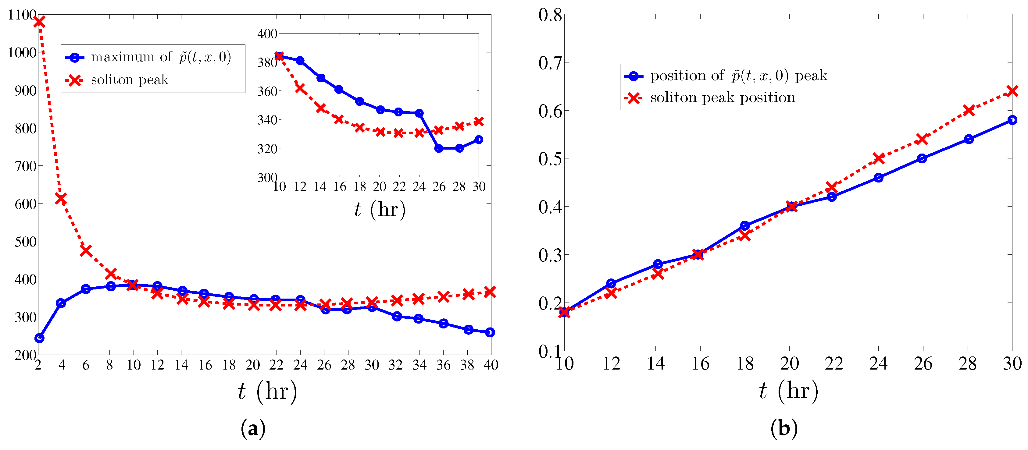
Using the soliton collective coordinates, we reconstruct the marginal vessel tip density and find its maximum value and the location thereof for all times . Figure 5 shows that the location of the soliton as predicted from the CCEs (38) and (39) compares very well with the marginal tip density obtained by ensemble averages (over 400 replicas) of the stochastic process during the 20 h time interval when boundaries do not affect soliton motion. There is a large discrepancy between the maximum marginal tip density as predicted by the soliton and by the stochastic process during the first 10 h of angiogenesis, which clearly marks the duration of the initial stage of soliton formation. After this stage, we note that the location of the maximum of the marginal tip density is very closely predicted by the location of the soliton peak as a function of time. However, the soliton density is noticeably wider than the ensemble averaged marginal density (see Figure 4). This is perhaps not so surprising. (i) The soliton is an approximate solution of Equation (28) for the marginal density that, in itself, is an approximation of (13) valid for large friction. A direct simulation of an overdamped Langevin model (1) with may provide better quantitative agreement with the soliton. Note that we do not have to select the velocity of the new tip branching from a given one in the overdamped case and that the injecting boundary condition (16) becomes given by (19) at [12]. With a few exceptions [5,6,7,9], most models in the literature are overdamped. (ii) The soliton is an approximate solution for an unbounded slab and the influence of the boundaries has to be eliminated by selecting the interval for spatial averaging. In view of Figure 5, we expect that the soliton approximation will improve if we increase the slab size so as to minimize the influence of boundaries.
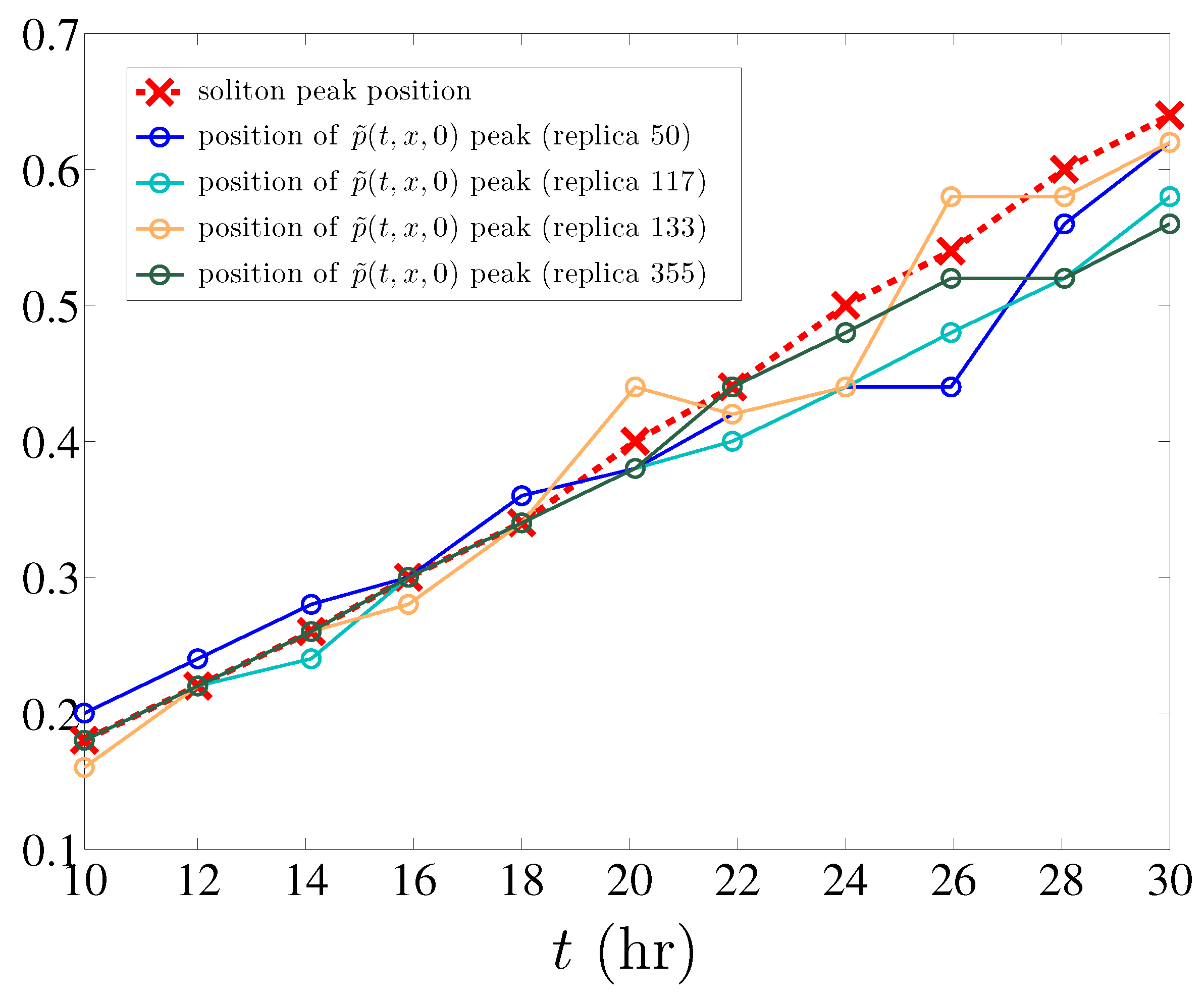
In addition, and as it also happens in the simpler model of angiogenesis without haptotaxis [12], the maximum marginal tip density of different single realizations of the stochastic process (defined by (11) with ) is well predicted by the position of the soliton peak density (see Figure 6). To explain this observation is an open problem.
7. Conclusions
In this paper, we have analyzed the influence of the haptotaxis mechanism in the first stages of tumor-induced angiogenesis following the Capasso–Morale model [7]. Blood circulation, secondary branching, remodeling and pruning of capillaries [22,23] are not considered in this mesoscopic model, nor are microscopic features such as cell size, shape and cellular mechanics [4,18]. The purpose of this paper is to show that the reduction of complex stochastic angiogenesis dynamics to the simpler soliton description of the angiogenic network allows incorporation of other transport mechanisms in addition to chemotaxis. As expected, including endothelial cell motion in an adverse fibronectin gradient through the extracellular matrix results in longer time scales for angiogenesis. As in previous work [9,10], there is a deterministic description associated to the full stochastic model: the density of active vessel tips satisfies an integrodifferential equation of Fokker–Planck type with a linear birth term and a nonlinear death (anastomosis) term. This equation is coupled to reaction–diffusion equations for the continuum fields (TAF, FN, MDE). Numerical simulations of the stochastic process show that, after an initial formation stage, the marginal tip density advances towards the tumor as a moving angiton whose longitudinal profile along the x-axis is soliton-like. Following the methodology explained in [11,12], we find an analytical formula for the soliton and collective coordinate equations that control shape and velocity of the soliton. When the soliton is about to reach the tumor, we need to study a different stage of soliton absorption by the tumor that is not contemplated in the present work. The detailed dynamics for TAF, FN and MDE as well as the chemotactic and haptotactic forces affecting vessel extension modify and influence the collective coordinate equations, which could be used to discuss possible anti-angiogenic strategies [28]. The description of angiogenesis in terms of soliton dynamics is confirmed by comparison with numerical simulations of the full stochastic model.
Acknowledgments
We thank Vincenzo Capasso, Bjorn Birnir and Boris Malomed for fruitful discussions. This work has been supported by the Ministerio de Economía y Competitividad grant MTM2014-56948-C2-2-P.
Author Contributions
Luis L. Bonilla designed the theoretical approach and wrote the paper, Manuel Carretero and Filippo Terragni performed the numerical simulations; the three authors analyzed the data and discussed the results. All authors have read and approved the final manuscript.
Conflicts of Interest
The authors declare no conflict of interest.
References
- Folkman, J. Tumor angiogenesis: Therapeutic implications. N. Engl. J. Med. 1971, 285, 1182–1186. [Google Scholar] [PubMed]
- Carmeliet, P.F. Angiogenesis in life, disease and medicine. Nature 2005, 438, 932–936. [Google Scholar] [CrossRef] [PubMed]
- Scianna, M.; Bell, J.; Preziosi, L. A review of mathematical models for the formation of vascular networks. J. Theor. Biol. 2013, 333, 174–209. [Google Scholar] [CrossRef] [PubMed]
- Heck, T.; Vaeyens, M.M.; van Oosterwyck, H. Computational models of sprouting angiogenesis and cell migration: Towards multiscale mechanochemical models of angiogenesis. Math. Model. Nat. Phenom. 2015, 10, 108–141. [Google Scholar] [CrossRef]
- Stokes, C.L.; Lauffenburger, D.A. Analysis of the roles of microvessel endothelial cell random motility and chemotaxis in angiogenesis. J. Theor. Biol. 1991, 152, 377–403. [Google Scholar] [CrossRef]
- Stokes, C.L.; Lauffenburger, D.A.; Williams, S.K. Migration of individual microvessel endothelial cells: stochastic model and parameter measurement. J. Cell Sci. 1991, 99, 419–430. [Google Scholar] [PubMed]
- Capasso, V.; Morale, D. Stochastic modelling of tumour-induced angiogenesis. J. Math. Biol. 2009, 58, 219–233. [Google Scholar] [CrossRef] [PubMed]
- Sun, S.; Wheeler, M.F.; Obeyesekere, M.; Patrick, C.W., Jr. Multiscale angiogenesis modeling using mixed finite element methods. Multiscale Model. Simul. 2005, 4, 1137–1167. [Google Scholar] [CrossRef]
- Bonilla, L.L.; Capasso, V.; Alvaro, M.; Carretero, M. Hybrid modeling of tumor-induced angiogenesis. Phys. Rev. E 2014, 90, 062716. [Google Scholar] [CrossRef] [PubMed]
- Terragni, F.; Carretero, M.; Capasso, V.; Bonilla, L.L. Stochastic model of tumor-induced angiogenesis: Ensemble averages and deterministic equations. Phys. Rev. E 2016, 93, 022413. [Google Scholar] [CrossRef] [PubMed]
- Bonilla, L.L.; Carretero, M.; Terragni, F.; Birnir, B. Soliton driven angiogenesis. Sci. Rep. 2016, 6, 31296. [Google Scholar] [CrossRef] [PubMed]
- Bonilla, L.L.; Carretero, M.; Terragni, F. Solitonlike attractor for blood vessel tip density in angiogenesis. Phys. Rev. E 2016, 94, 062415. [Google Scholar] [CrossRef] [PubMed]
- Anderson, A.R.A.; Chaplain, M.A.J. Continuous and discrete mathematical models of tumor-induced angiogenesis. Bull. Math. Biol. 1998, 60, 857–900. [Google Scholar] [CrossRef] [PubMed]
- Plank, M.J.; Sleeman, B.D. Lattice and non-lattice models of tumour angiogenesis. Bull. Math. Biol. 2004, 66, 1785–1819. [Google Scholar] [CrossRef] [PubMed]
- Stéphanou, A.; McDougall, S.R.; Anderson, A.R.A.; Chaplain, M.A.J. Mathematical modelling of the influence of blood rheological properties upon adaptative tumour-induced angiogenesis. Math. Comput. Model. 2006, 44, 96–123. [Google Scholar] [CrossRef]
- Chaplain, M.A.J.; McDougall, S.R.; Anderson, A.R.A. Mathematical modelling of tumor-induced angiogenesis. Annu. Rev. Biomed. Eng. 2006, 8, 233–257. [Google Scholar] [CrossRef] [PubMed]
- Gardiner, C.W. Stochastic Methods. A Handbook for the Natural and Social Sciences, 4th ed.; Springer: Berlin/Heidelberg, Germany, 2010. [Google Scholar]
- Bauer, A.L.; Jackson, T.L.; Jiang, Y. A cell-based model exhibiting branching and anastomosis during tumor-induced angiogenesis. Biophys. J. 2007, 92, 3105–3121. [Google Scholar] [CrossRef] [PubMed]
- Alber, M.S.; Chen, N.; Glimm, T.; Lushnikov, P.M. Multiscale dynamics of biological cells with chemotactic interactions: From a discrete stochastic model to a continuous description. Phys. Rev. E 2006, 73, 051901. [Google Scholar] [CrossRef] [PubMed]
- Pries, A.R.; Secomb, T.W.; Gaehtgens, P. Structural adaptation and stability of microvascular netwoks: Theory and simulation. Am. J. Physiol. Heart Circ. Physiol. 1998, 275, H349–H360. [Google Scholar]
- Pries, A.R.; Secomb, T.W. Control of blood vessel structure: insights from theoretical models. Am. J. Physiol. Heart Circ. Physiol. 2005, 288, H1010–H1015. [Google Scholar] [CrossRef] [PubMed]
- McDougall, S.R.; Anderson, A.R.A.; Chaplain, M.A.J. Mathematical modelling of dynamic adaptive tumour-induced angiogenesis: Clinical implications and therapeutic targeting strategies. J. Theor. Biol. 2006, 241, 564–589. [Google Scholar] [CrossRef] [PubMed]
- Ronellenfitsch, H.; Katifori, E. Global Optimization, Local Adaptation, and the Role of Growth in Distribution Networks. Phys. Rev. Lett. 2016, 117, 138301. [Google Scholar] [CrossRef] [PubMed]
- Ronellenfitsch, H.; Lasser, J.; Daly, D.C.; Katifori, E. Topological Phenotypes Constitute a New Dimension in the Phenotypic Space of Leaf Venation Networks. PLoS Comput. Biol. 2016, 11, e1004680. [Google Scholar] [CrossRef] [PubMed]
- Levine, H.A.; Pamuk, S.; Sleeman, B.D.; Nilsen-Hamilton, M. Mathematical modeling of the capillary formation and development in tumor angiogenesis: Penetration into the stroma. Bull. Math. Biol. 2001, 63, 801–863. [Google Scholar] [CrossRef] [PubMed]
- Carpio, A.; Duro, G. Well posedness of an angiogenesis related integrodifferential diffusion model. Appl. Math. Model. 2016, 40, 5560–5575. [Google Scholar] [CrossRef]
- Carpio, A.; Duro, G.; Negreanu, M. Constructing solutions for a kinetic model of angiogenesis in annular domains. Appl. Math. Model. 2017, 45, 303–322. [Google Scholar] [CrossRef]
- Orme, M.E.; Chaplain, M.A.J. Two-dimensional models of tumour angiogenesis and anti-angiogenesis strategies. IMA J. Math. Appl. Med. Biol. 1997, 14, 189–205. [Google Scholar] [CrossRef] [PubMed]
Figure 1.
Comparison between the vessel networks of two replicas after 36 h for the model with chemotaxis (a), and for the model with chemo and haptotaxis (b). The TAF level curves have also been depicted.
Figure 1.
Comparison between the vessel networks of two replicas after 36 h for the model with chemotaxis (a), and for the model with chemo and haptotaxis (b). The TAF level curves have also been depicted.
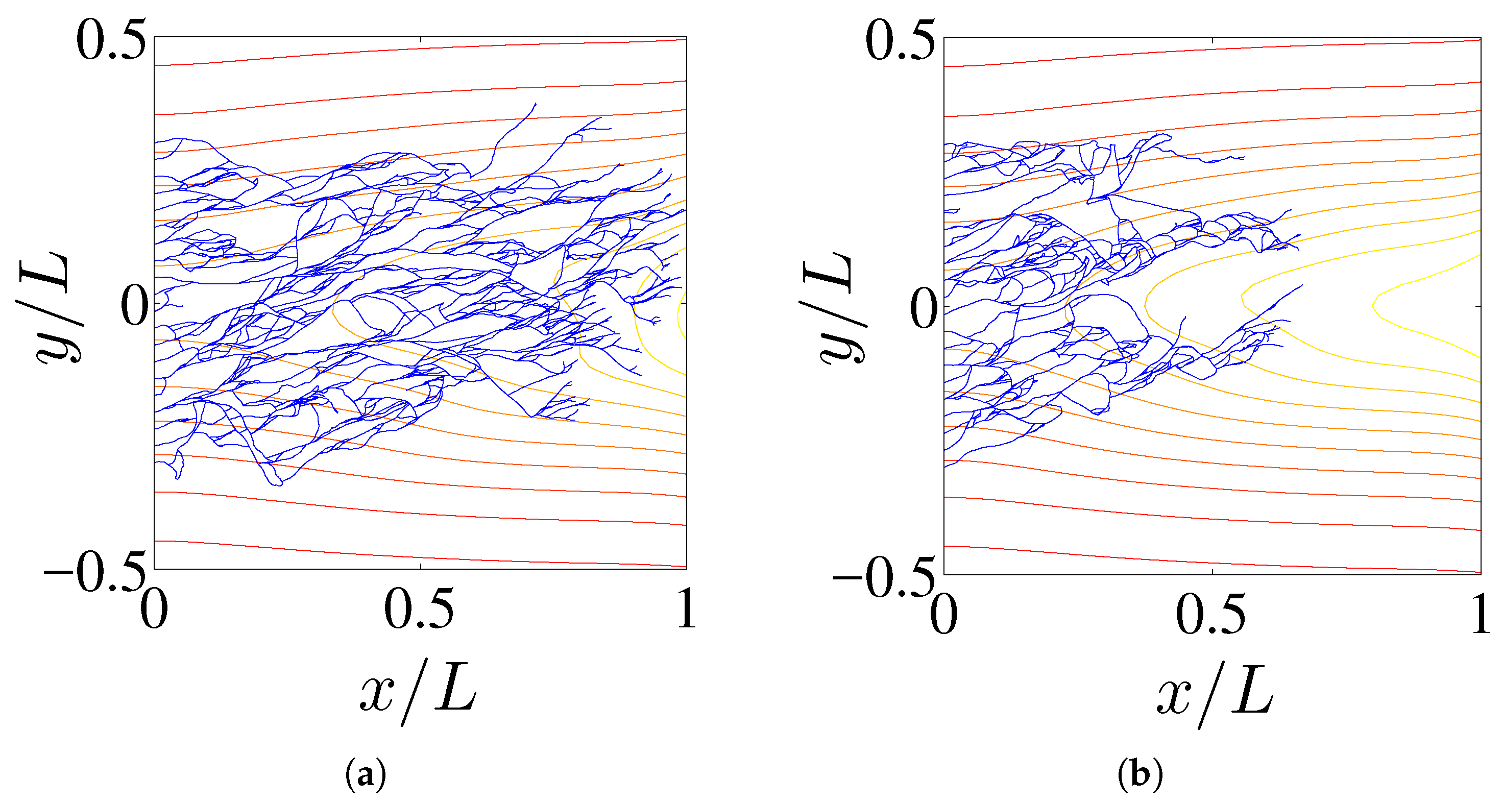
Figure 2.
Effect of haptotaxis on the profile of (calculated by ensemble average over 400 realizations) at times 24 h (a) and 36 h (b). Solid line: profile including haptotaxis, dashed line: profile without haptotaxis.
Figure 2.
Effect of haptotaxis on the profile of (calculated by ensemble average over 400 realizations) at times 24 h (a) and 36 h (b). Solid line: profile including haptotaxis, dashed line: profile without haptotaxis.
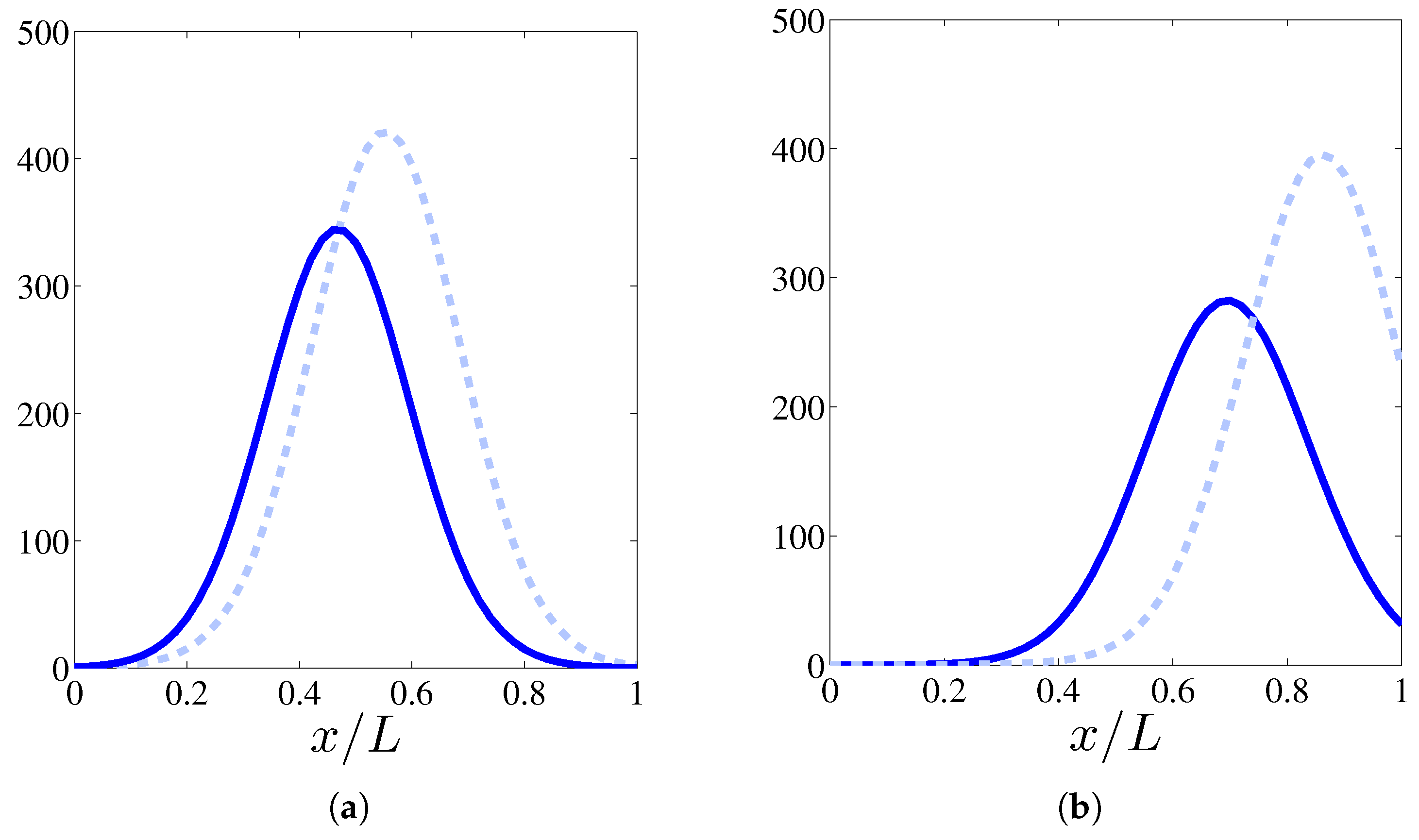
Figure 3.
Normalized consumption of fibronectin given by , cf. Equation (8), by the angiogenic network calculated for a single replica in panels (a) 24 h and (b) 36 h. Panels (c) and (d) correspond to (a) and (b) but now the consumption has been calculated by ensemble averages over 400 replicas.
Figure 3.
Normalized consumption of fibronectin given by , cf. Equation (8), by the angiogenic network calculated for a single replica in panels (a) 24 h and (b) 36 h. Panels (c) and (d) correspond to (a) and (b) but now the consumption has been calculated by ensemble averages over 400 replicas.
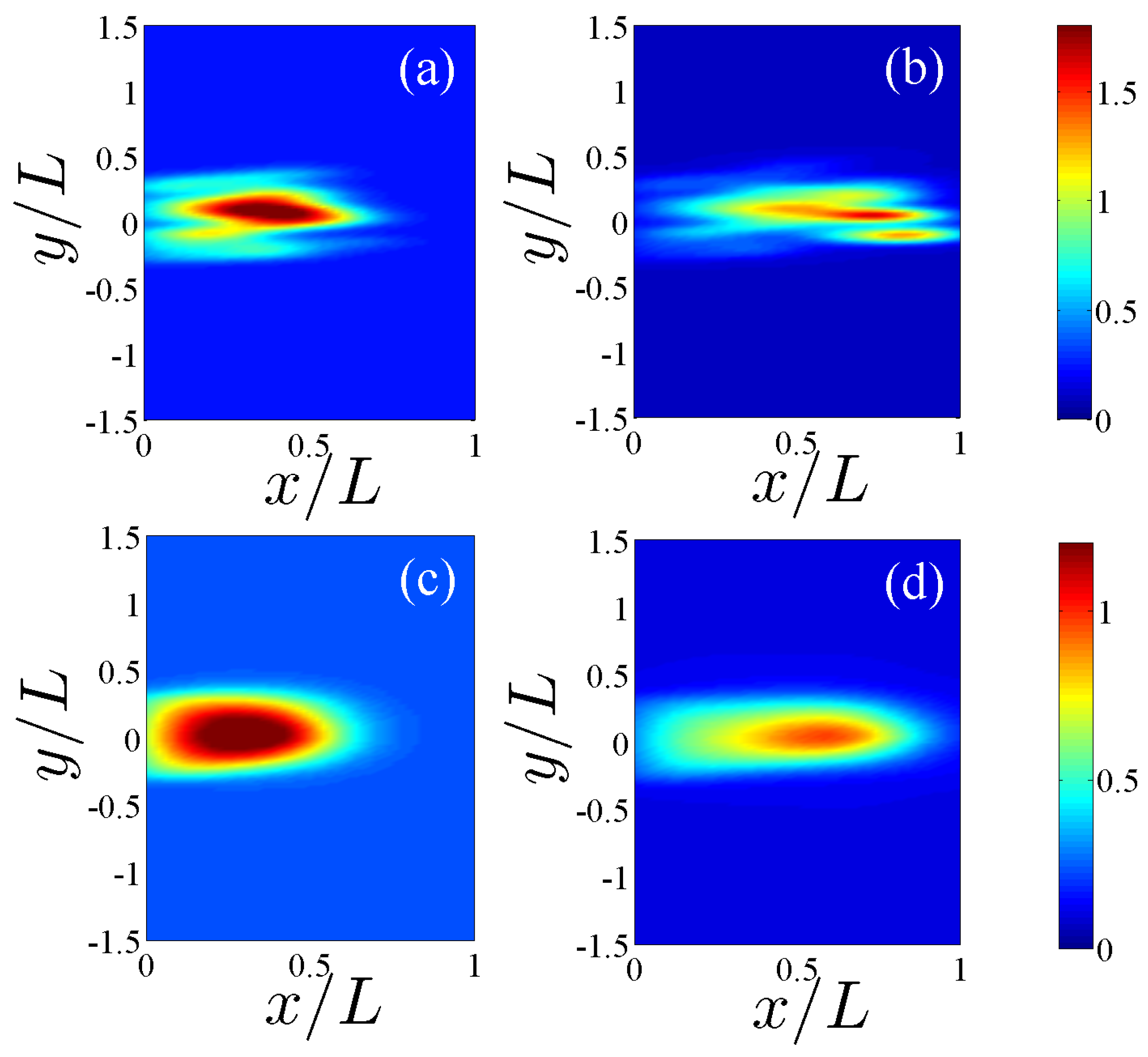
Figure 4.
Comparison between the profile of (solid line, calculated by ensemble average over 400 realizations) and its reconstruction from the soliton collective coordinates (dashed line) at times: (a) 12 h; (b) 18 h; (c) 24 h; (d) 30 h.
Figure 4.
Comparison between the profile of (solid line, calculated by ensemble average over 400 realizations) and its reconstruction from the soliton collective coordinates (dashed line) at times: (a) 12 h; (b) 18 h; (c) 24 h; (d) 30 h.
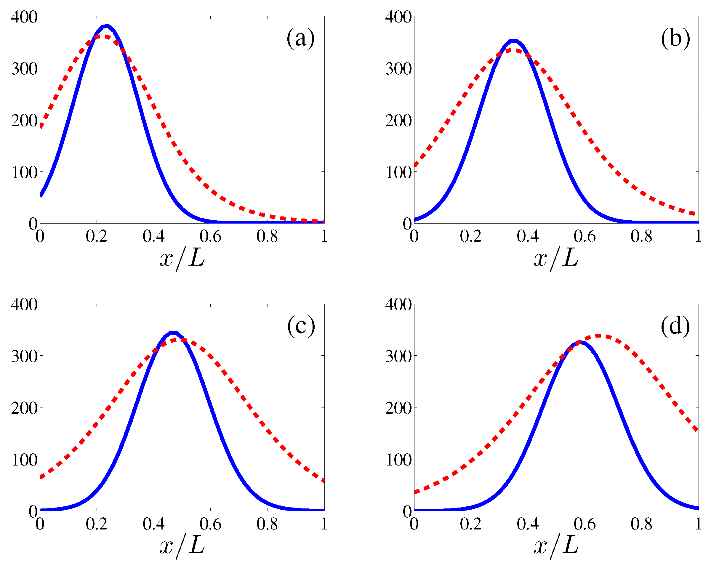
Figure 5.
Comparison between the maximum value of (calculated by ensemble average over 400 realizations) and its value as predicted by soliton collective coordinates. (a): evolution of the maximum value of the marginal tip density (relative error smaller than 5.8% for times between 10 and 30 h); (b): evolution of the position of the maximum marginal tip density on (at h, the absolute error is the space step in the numerical method, ; at h, the error is ). We have used an anastomosis coefficient .

Figure 6.
Position of the soliton peak compared to that of the maximum marginal tip density for different replicas of the stochastic process.
Figure 6.
Position of the soliton peak compared to that of the maximum marginal tip density for different replicas of the stochastic process.

Table 1.
Units to non-dimensionalize the model equations.
| x | v | t | C | f | m |
|---|---|---|---|---|---|
| L | |||||
| mm | m/h | h | mol/m | mol/m | mol/m |
| 2 | 40 | 50 |
Table 2.
Parameters appearing in the model equations, taken from [10]. Here, .
Table 2.
Parameters appearing in the model equations, taken from [10]. Here, .
| h | m/s | m | |||
| 8.5 | 4.035 | 1.538 | 2400 | 800 | 4 |
© 2017 by the authors. Licensee MDPI, Basel, Switzerland. This article is an open access article distributed under the terms and conditions of the Creative Commons Attribution (CC BY) license (http://creativecommons.org/licenses/by/4.0/).
Share and Cite
MDPI and ACS Style
Bonilla, L.L.; Carretero, M.; Terragni, F. Ensemble Averages, Soliton Dynamics and Influence of Haptotaxis in a Model of Tumor-Induced Angiogenesis. Entropy 2017, 19, 209. https://doi.org/10.3390/e19050209
AMA Style
Bonilla LL, Carretero M, Terragni F. Ensemble Averages, Soliton Dynamics and Influence of Haptotaxis in a Model of Tumor-Induced Angiogenesis. Entropy. 2017; 19(5):209. https://doi.org/10.3390/e19050209
Chicago/Turabian StyleBonilla, Luis L., Manuel Carretero, and Filippo Terragni. 2017. "Ensemble Averages, Soliton Dynamics and Influence of Haptotaxis in a Model of Tumor-Induced Angiogenesis" Entropy 19, no. 5: 209. https://doi.org/10.3390/e19050209
Note that from the first issue of 2016, this journal uses article numbers instead of page numbers. See further details here.